Megamap: flexible representation of a large space embedded with nonspatial information by a hippocampal attractor network

The megamap is a quasi-continuous attractor network built on the experimental fact that each place cell has multiple, irregularly spaced place fields in a large environment. This flexibility allows the megamap to seamlessly cover much larger environments than standard rigid continuous attractor models. The megamap has additional inherent properties, such as robustness to degraded inputs and ease of storing nonspatial information, that render it suitable as a basic building block for modeling hippocampal activity.

Abstract

The problem of how the hippocampus encodes both spatial and nonspatial information at the cellular network level remains largely unresolved. Spatial memory is widely modeled through the theoretical framework of attractor networks, but standard computational models can only represent spaces that are much smaller than the natural habitat of an animal. We propose that hippocampal networks are built on a basic unit called a “megamap,” or a cognitive attractor map in which place cells are flexibly recombined to represent a large space. Its inherent flexibility gives the megamap a huge representational capacity and enables the hippocampus to simultaneously represent multiple learned memories and naturally carry nonspatial information at no additional cost. On the other hand, the megamap is dynamically stable, because the underlying network of place cells robustly encodes any location in a large environment given a weak or incomplete input signal from the upstream entorhinal cortex. Our results suggest a general computational strategy by which a hippocampal network enjoys the stability of attractor dynamics without sacrificing the flexibility needed to represent a complex, changing world.

NEW & NOTEWORTHY

The megamap is a quasi-continuous attractor network built on the experimental fact that each place cell has multiple, irregularly spaced place fields in a large environment. This flexibility allows the megamap to seamlessly cover much larger environments than standard rigid continuous attractor models. The megamap has additional inherent properties, such as robustness to degraded inputs and ease of storing nonspatial information, that render it suitable as a basic building block for modeling hippocampal activity.

an attractor network is a widely used theoretical framework for constructing neural models of spatial, declarative, and episodic memory. Attractor dynamics arise naturally in models of recurrent neural networks with Hebbian-type associative synaptic plasticity (Cerasti and Treves 2013; Kali and Dayan 2000; Knierim and Zhang 2012). The resulting attractor networks exhibit emergent properties desirable for memory storage, such as full recalls from partial cues and robustness against noise and damage (Hopfield 1982; Marr 1971; McNaughton and Nadel 1990), and they have become increasingly useful for neurophysiology by offering a practical framework for experimental design and data interpretation (Peyrache et al. 2015; Stella et al. 2012; Yoon et al. 2013).

The hippocampus, especially the CA3 area with its prominent recurrent collaterals and proposed role in associative memory (Johnston and Amaral 1998; Nakazawa et al. 2004), has long been modeled as a discrete attractor network representing nonspatial information and as a continuous attractor network representing space (Knierim and Zhang 2012; Leutgeb and Leutgeb 2007; Rolls 2007). The latter class of models has largely been built on the seminal theory commonly referred to as the multichart model (Samsonovich and McNaughton 1997; Tsodyks 1999). The fundamental idea is that a given spatial environment is represented by a cognitive map (chart) in which each place cell is located at its single place field center (Fig. 1A). The strength of recurrent connections then decays exponentially with distance between cells on the chart, consistent with Hebbian plasticity. The chart has become a useful convention by which one may visualize place cell activity as a localized activity bump on the chart centered at the animal's current location. Moreover, the model offers a plausible explanation for experimental data, such as the relative stability of place cell activity in the CA3 compared with that in the CA1 (Lee et al. 2004; Vazdarjanova and Guzowski 2004). Numerous studies have used the chart as a building block, modeling additional biological mechanisms and multiple charts to capture various phenomena, e.g., global remapping (Samsonovich and McNaughton 1997), partial remapping (Stringer et al. 2004), rate remapping (Rennó-Costa et al. 2014; Solstad et al. 2014), and incorporation of nonspatial information (Rolls et al. 2002). Other studies have shown how the chart may self-organize (Cerasti and Treves 2013; Kali and Dayan 2000; Stringer et al. 2002) and have generalized the attractor to model context dependence (Doboli et al. 2000).

Fig. 1.

Basic models of place cell representations. In this schematic, 16 place cells represent a large uniform space, where cell numbers are placed at respective place field centers, and the fields of cells 1–4 are additionally indicated by color. A: models of single-peaked attractor networks assume each cell represents at most one location. This rigid representation limits the environmental size, because it is unclear how the network would represent new locations after all cells have been used. B: one possible remedy is to partition the region, treating each subregion as a distinct environment in which each cell has at most one place field. The resulting representation is piecewise rigid with artificial boundaries between subregions. C: place cells are flexibly recombined for the flexible representation on which the megamap is built. A single cognitive map without artificial boundaries or size limitations represents the large space. D: we construct a benchmark model for the flexible representation by assuming the number of place fields (k) for a given cell in the represented region follows the Poisson distribution (Eq. 1). The average field density is given by λ = −ln(0.8) m⁻² ≈ 0.22 m⁻².

The ideal chart is single peaked, i.e., each place cell exhibits a single place field within a single environment. This simplification, which is common to most attractor models, is justifiable in a small, standard environment (∼1 m²), in which a majority of place cells exhibit no more than one place field. The chart does not extend naturally to large environments. Since each cell appears only once on the chart, it can only represent a small area before all cells are used (McNaughton et al. 2006). Assuming ∼20% of cells in the CA3 have place fields within a 1-m² environment, the entire CA3 could represent at most 5 m², a much smaller area than the foraging range of a rat (Davis 1953; Innes and Skipworth 1983; Lambert et al. 2008; Taylor 1978).

One possibility is that place fields scale with the environmental size (Muller et al. 1987; O'Keefe and Burgess 1996). A scaled representation would certainly increase the capacity of any cognitive map, but it would also coarsen the map's spatial resolution. Another possibility is that the animal partitions the environment, treating each subregion as a distinct environment represented by a distinct chart (Fig. 1B). This simple model removes size limitations by imposing artificial boundaries on a seemingly continuous space, and it is unclear how such a partitioned cognitive map might self-organize in a novel environment. Furthermore, while the boundaries between charts may be difficult to detect (Samsonovich 1998), they have not been apparent in recent experiments conducted in large environments (Fenton et al. 2008; Park et al. 2011; Rich et al. 2014). Rather, these experimental data seem to indicate that the animal represents a larger than standard environment through a single cognitive map in which many place cells exhibit multiple, irregularly spaced place fields. Thus an attractor network based on a single-peaked code is appropriate for modeling head-direction cells (Peyrache et al. 2015; Redish et al. 1996; Seelig and Jayaraman 2015; Skaggs et al. 1995; Zhang 1996), grid cells within a module (McNaughton et al. 2006; Yoon et al. 2013), and even place cells representing a small environment (McNaughton et al. 2006; Samsonovich and McNaughton 1997; Tsodyks 1999); but it becomes unnatural for place cells representing a large environment.

We offer a more natural theoretical framework for an attractor network representing a large space. We propose that hippocampal networks are built on a megamap, or a single, quasi-continuous attractor map in which place cells with structured recurrent connections are flexibly recombined to represent a large space (Fig. 1C). The megamap's underlying place code, which we refer to as the flexible representation, is based directly on experimental data (Fenton et al. 2008; Park et al. 2011; Rich et al. 2014). However, the megamap is the first model to explicitly examine the structure and properties of an attractor network built on this flexible representation. Our focus in this study is to present the megamap as a basic unit of a cognitive map by elucidating the structure of the optimal recurrent connections, demonstrating the novel manner in which an activity bump on the megamap may be visualized, and comparing the properties of the megamap with those of the alternative single-peaked chart. The model also reveals two emergent properties of the multipeaked attractor network: its adaptation to environmental changes by recombining learned memories, and its incorporation of nonspatial information at no additional cost. We close by discussing experimental predictions and implications of the megamap.

MATERIALS AND METHODS

Poisson distribution of place fields on the megamap.

The megamap represents a large space through flexible recombinations of place cells. In other words, each cell in the megamap has multiple, irregularly spaced place fields, and there is no spatial correlation among place field pairs. We construct a benchmark model by setting place fields according to the Poisson distribution, for which the probability that a given place cell has k place fields in a region of area A is given by

$$P\left(k\right)=e^{-\lambda A}{\left(\lambda A\right)}^k/k!$$ (1)

The single parameter, λ, is the average number of place fields per unit area for a single cell. By using Eq. 1 with k = 0, λ = −ln[P(0)]/A, where P(0) is the proportion of silent cells in a region of area A. Unless otherwise specified, we set λ = −ln(0.8)/(1 m²) ≈ 0.22 m⁻². This estimate is derived from the observation that roughly 80% of CA3 place cells are silent in standard recording enclosures (A ∼ 1 m²) (Alme et al. 2014; Vazdarjanova and Guzowski 2004). For simplicity, we assume λ is constant for all cells, rather than variable (Rich et al. 2014). The place fields of each cell are centered at random locations throughout the environment.

Flexible representation of a large space.

We first consider the implications of a flexible, multipeaked place code without modeling an underlying dynamical system. Rather, we initially consider a flexible representation in which each place cell exhibits Gaussian place fields distributed according to the Poisson distribution.

In this context the representational capacity refers to the number of locations uniquely encoded on the cognitive map. For the single-peaked and flexible representations, we estimate the representational capacity by computing the number of unique subsets of place cells that may be co-active in an activity bump. We compute the analogous measure of the representational capacity for grid cells as done by Fiete et al. (2008). Consider a population of N grid cells divided evenly among M modules. Unique subsets of co-active grid cells within a module appear to encode distinct phases of the animal's location with respect to the period (spacing) of the module. Since there is a rigid spatial relation among phases within a module (Yoon et al. 2013), a single module can uniquely encode N/M phases, analogous to the single-peaked place code. The entire population may encode the animal's actual location through a unique set of phases over all modules, bounding the representational capacity by C_grid ≤ (N/M)^M. [One may compute the capacity in terms of distance uniquely represented by determining the uncertainty of a downstream neural population in reading the location encoded by place cells or the phase encoded by grid cells (Fiete et al. 2008). Assuming a similar uncertainty for either population, the qualitative results would be unchanged.]

In this report the spatial resolution refers to the least mean squared error between the animal's location [x = (x₁, x₂)] and the decoded location [x̂ = (x̂₁, x̂₂)] given any scheme for decoding the stochastic spike vector s, whose elements are the number of spikes for each place cell in the time window T. The spatial resolution is determined analytically by computing the Fisher information (Kay 1993). Regardless of the place field distribution, element (i, j) of the 2 × 2 Fisher information matrix carried by N place cells is given by

$${\left[\text{F}\left(x\right)\right]}_{ij}=T{\displaystyle {\sum }_{n=1}^N\frac{\left[\frac{\partial }{\partial x_i}{r}_n\left(x\right)\right]\left[\frac{\partial }{\partial x_j}{r}_n\left(x\right)\right]}{r_n\left(x\right)}},$$ (2)

where the average firing rate of cell n with place field centers {c_nm}_m=1^M_n and peak firing rate a is given by

$$r_n\left(x\right)=a{\displaystyle {\sum }_{m=1}^{M_n}\text{exp}\hspace{0.17em}\left(\frac{-{\left|x-c_{nm}\right|}^2}{2{\sigma }^2}\right)}$$ (3)

Neglecting the rare overlapping place fields of individual cells [which create slight variations in F(x) over the region], only one term of the summation in Eq. 3 is nonzero. This permits Eq. 2 to be simplified to a single summation over all place fields of all cells. Assuming x is at least a place field width from any boundary, in the limit of a large population,

$${\left[\text{F}\left(x\right)\right]}_{ij}=\frac{Ta{N}_{\text{flds}}}{A}{\displaystyle \iint \frac{\left(\frac{\partial }{\partial y_i}h\left(y\right)\right)\left(\frac{\partial }{\partial y_j}h\left(y\right)\right)}{h\left(y\right)}}dy$$

$$=\frac{Ta\rho }{{\sigma }^4}{\displaystyle \iint y_i{y}_j}h\left(y\right)dy,$$

where $h\left(y\right)=\exp [-{\left|y\right|}^2/\left({2\sigma }^2\right)],$ A is the area of the region, N_flds is the number of place fields for the entire population, and ρ = N_flds/A is the density of all place fields in the population. Therefore,

$$\text{F}\left(x\right)=\left(2\pi Ta\rho \right)\left(\begin{array}{cc}1& 0\\ 0& 1\end{array}\right).$$

Finally, the expected value of the squared error is bounded below by

$$\min \hspace{0.17em}\text{E}\left[{\left|\hat{\mathbf{x}}-\mathbf{x}\right|}^2\right]=\min \hspace{0.17em}\text{trace}\left(\mathrm{cov}\left(\hat{\mathbf{x}}\right)\right)=\text{trace}\left({\mathbf{F}}^{-1}\right)=1/\left(\pi Ta\rho \right)$$ (4)

by the Cramér-Rao lower bound, assuming x̂ is an unbiased estimator (E[x̂] = x).

An upstream neuronal population can theoretically decode the stochastic spike vector s to obtain this optimal accuracy (Eq. 4) by computing the maximum likelihood estimate (MLE), which has biologically plausible implementations (Jazayeri and Movshon 2006; Pouget et al. 1998). The MLE is given by

$$\begin{array}{c}\hat{\mathbf{x}}=\underset{y}{\text{argmax}}\hspace{0.17em}\ln \left[P\left(s|y\right)\right]=\underset{y}{\text{argmax}}\hspace{0.17em}\ln \left[{\displaystyle \prod _{n=1}^{N}P\left(s_n|y\right)}\right]\\ =\underset{y}{\text{argmax}}{\displaystyle {\sum }_{n=1}^N\left\{s_n\hspace{0.17em}\ln \left[r_n\left(y\right)T\right]-r_n\left(y\right)T\right\}}\end{array}$$ (5)

assuming the place cell spike trains are independent Poisson processes such that

$$\begin{array}{c}\begin{array}{l}P\left(s_n|\mathbf{x}\right)=e^{-r_n\left(x\right)T}{\left(r_n\left(\mathbf{x}\right)T\right)}^{s_n}/s_n!\\ \end{array}\\ \end{array}$$

is the probability that cell n has s_n spikes in the time window T given the animal's location x.

We numerically test the agreement between the analytical spatial resolution (Eq. 4) and the mean squared error in the MLE (Eq. 5) for the standard, scaled, and flexible place cell representations (see Fig. 4). For the standard and scaled representations, each of N place cells has a single place field, where the place field centers are distributed uniformly throughout the region. The place field width is held constant for the standard representation, while the place field width (as controlled by σ in Eq. 3) for the scaled representation increases with the environmental area such that the number of co-active cells at any location is constant. For the flexible representation, which is used to generate the megamap, place fields of each cell follow the Poisson distribution (Eq. 1).

Fig. 4.

Spatial resolution, as quantified by the least mean squared error (LMSE) between the animal's position and the position decoded from the stochastic spikes of place cells with idealized Gaussian place fields (Eq. 3). A: the spatial resolution grows linearly with the area of the represented region if each place cell has exactly one place field, whether the place field size is constant (Standard Rep.) or grows with the environmental size (Scaled Rep.). In contrast, the LMSE is constant for any area given the Poisson distribution of place fields used for the megamap (Flexible Rep.). The apparent advantage of the single-peaked codes over the flexible representation when A < 1/λ is an artifact, since many cells in the flexible representation are silent in these small regions. The maximum likelihood estimates (MLEs; Eq. 5) approximate the LMSE (black; Eq. 4), as expected since the MLEs are unbiased estimators. (The mean error along either dimension is negligible: −0.0080 ± 0.0076 cm for the single-peaked place code and 0.0006 ± 0.0063 cm for the megamap.) B: the standard deviation of the Gaussian place fields (Eq. 3) grows with the environmental area only for the scaled representation. C: the number of co-active place cells at any single position is constant for the scaled and flexible representations but decreases for the standard representation, since the number of cells (N) is constant. For all simulations presented, N = 22,500, T = 250 ms, λ = −ln(0.8) m⁻², and a = 15 Hz (see materials and methods for more details).

We place the animal at 50 random locations (not necessarily locations on which place fields are centered) at least 20 cm from any boundary of the region. At each location we compute the MLE for each of 50 stochastic spike vectors, s. We solve Eq. 5 by finding the maximizer over the vertices of a square grid of length 10 cm and pixel size 0.05 × 0.05 cm² centered at the animal's true location. We also perform a coarse exhaustive search with a pixel size of 4 × 4 cm² over the entire region to catch outliers. We then plot the mean squared error between the MLE and the animal's location, averaged over all 2,500 iterates. This process is repeated over regions varying in size with T = 250 ms, N = 22,500, a = 15 Hz, and σ = 5 cm.

Dynamical system of the megamap.

We examine how an associative network of place cells may contribute to the formation and stability of the activity bump on the megamap by simulating a standard firing rate model (Li and Dayan 1999; Wilson and Cowan 1972) consisting of a network of N place cells with recurrent excitation, global feedback inhibition, and external input. The state vector, u ∈ ℝ^N×1, loosely represents the depolarization of each place cell and is governed by

$$\tau {u\prime }^{}\left(t\right)=-u\left(t\right)+Wf\left(t\right)-w^{\mathrm{I}}{f}^{\mathrm{I}}\left(t\right)1+I\left(t\right),$$ (6)

where τ = 10 ms and 1 ∈ ℝ^N×1 denotes a vector of all ones.

The recurrent excitation, Wf, provides the internal network drive. The weight matrix, W ∈ ℝ^N×N, describes the strength of connections among place cells. The activity vector, f ∈ ℝ^N×1, represents the firing rate of place cells and depends on the state through the threshold linear gain function,

$$f=g\left(u\right)=f_{\text{peak}}{\left[u\right]}_{+},$$ (7)

where [·]₊ = max(·, 0) and f_peak = 15 Hz. We use a threshold linear gain function because of its simplicity for analysis, but similar qualitative results would be obtained using a sigmoid gain function.

All interneurons are modeled as a single inhibitory unit providing global feedback inhibition so that only the external input and recurrent hippocampal input provide a spatial signal. Future versions of the model may incorporate a weak spatial signal carried by hippocampal theta cells (Kubie et al. 1990). The activity of the inhibitory unit, f^I, depends on the total network activity through the threshold linear gain function,

$$f^{\text{I}}=g^{\text{I}}\left(f\right)={\left[{\mathbf{1}}^{\mathbf{\text{T}}}\mathbf{\text{f}}-\theta \right]}_{+}.$$

The inhibitory threshold is set to 90% of the total desired activity (Eq. 9). Explicitly, θ = 0.9·1^Tf̄(x), which is constant for all x. The inhibitory activity is scaled by w^I to provide global inhibition to all place cells, controlling the overall network activity.

The external input, I ∈ ℝ^N×1, carries sensory information about the animal's location or self-motion. We model the collective effect of the various external inputs into the hippocampus as a Gaussian shaped pattern that peaks at the animal's location on the megamap, and we focus our attention on the inherent dynamics of the attractor network. The external input into cell n when the animal is at location x is modeled by

$$I_n\left(x;I_{peak}\right)=I_{peak}{\displaystyle {\sum }_{m=1}^{M_n}\exp \hspace{0.17em}\left(\frac{-{\left|c_{nm}-x\right|}^2}{2{\sigma }_u^2}\right)}$$ (8)

so that the input peaks at the place field centers of cell n, {c_nm}_m=1^M_n. The parameter σ_u is set such that the external input and the network state have the same width.

We integrate the dynamical system using the staggered Euler scheme (Hines 1984) with a time step of 0.1 ms. We consider the state to be an equilibrium state if its relative change over 50 ms is less than 10⁻⁶. The activity of an ensemble of hippocampal place cells can be decoded to predict the animal's perceived location (Brown et al. 1998; Davidson et al. 2009; Wilson and McNaughton 1993; Zhang et al. 1998). We decode the network activity through a process called maximum likelihood Euclidean distance decoding (Cerasti and Treves 2013; Rolls et al. 1997). We find the location, x̂, at which the desired activity, f̄(x̂) (Eq. 9), best approximates the network activity, f(t). Explicitly, the location encoded by the activity bump satisfies

$$\hat{\mathbf{x}}\left(t\right)={\text{argmin}}_x\Vert f\left(t\right)-\overline{f}\left(x\right)\Vert /\Vert \overline{f}\left(x\right)\Vert .$$

We compute x̂ by first finding x̂¹, the minimizer over all vertices in the region on which a place field is centered. Since the activity bump may encode locations between place field centers, we then refine the search about x̂¹. The final decoded location is the minimizer over the vertices of a square grid of width d with pixel size 0.1 × 0.1 cm² centered at x̂¹, where d is the distance between neighboring place field centers along either dimension.

Construction of the ideal megamap.

We construct a benchmark model to determine whether a network with a flexible representation can exhibit stable, Gaussian-like place fields. Unless otherwise specified, the megamap represents a 3 × 3-m² region and comprises 11,240 place cells (9,731 active cells and 1,509 silent cells).

We first set the desired place field centers. The number of place fields for each cell n (M_n) is set according to the Poisson distribution (Eq. 1) with density λ = −ln(0.8) m⁻² ≈ 0.22 m⁻². Each place field center {c_nm}_m=1^M_n is then assigned to a random vertex of a rectangular grid over the entire region such that exactly one field is centered at each vertex, resulting in a place field center each 4 cm².

When the external input is spatially tuned, the depolarization of a place cell with a single place field should ideally decay as a Gaussian with the distance between the place field center and the animal's location. Under the simplification that multiple place fields of a cell sum linearly, the desired activity of a given cell n when the animal is at location x is given by

$${{\overline{f}}_n}_{}\left(\mathbf{x}\right)={\displaystyle {\sum }_{m=1}^{M_n}{f}_{\text{tune}}\left(\left|c_{nm}-\mathbf{x}\right|\right)},$$ (9)

where the state and activity tuning curves are respectively given by

$$u_{\text{tune}}\left(d\right)=\left(1+u_0\right)\exp \left(\frac{-d^2}{2{\sigma }_u^2}\right)-u_0\hspace{1em}\text{and}\hspace{1em}{f}_{\text{tune}}\left(d\right)=g\left(u_{\text{tune}}\left(d\right)\right).$$

The gain function, g(u), is defined in Eq. 7. The parameter u₀ = 0.2 permits subthreshold depolarization, and the parameter σ_u = 5.94 cm is set such that f_tune best approximates a Gaussian tuning curve with a standard deviation of 5 cm, as expected for place cells in the dorsal hippocampus (Muller 1996).

We set the inhibitory weight (w^I) and recurrent weights among place cells (W) such that the desired activity vectors (Eq. 9) correspond to fixed points of the dynamical system (Eq. 6) when the external input is given by Eq. 8 with I_peak = 0.3. For the resting state of a place cell to be −u₀, the inhibitory weight is given by the explicit expression,

$$w^{\text{I}}=u_0/\left(1^{\text{T}}\overline{f}-\theta \right).$$

Since the summation of the ideal network activity (1^Tf̄) is constant throughout the region (within a place field width of a boundary), w^I is independent of the animal's location.

The optimal recurrent weights onto a given cell j are initialized to zero and set iteratively through the delta rule,

$$\Delta W_{jk}=s{\displaystyle {\sum }_i\left[f_j^{\text{proj}}\left(x^i\right)-{{\overline{f}}_{}}_j\left(x^i\right)\right]}{{\overline{f}}_k}_{}\left(x^i\right),$$ (10)

where xⁱ are all vertices, or locations at which a place field is centered, within the set learning region. Unless otherwise specified, the learning region is any location at least 20 cm from any boundary of the environment. The projected activity vector is given by

$$f^{\text{proj}}\left(x\right)=g(W\overline{f}(x)-w^{\text{I}}{g}^{\text{I}}\left(\overline{f}\left(x\right)\right)1+\text{I}\left(x;0.3\right)).$$

The resulting weights may be considered optimal since f̄(xⁱ) corresponds to a fixed point of Eq. 6 if f̄(xⁱ) = f^proj(xⁱ), and the delta rule minimizes the least squared error between the projected and desired activity vectors for each cell j. The learning rate (s) is sufficiently small such that f^proj(xⁱ) → f̄(xⁱ) smoothly. No sparsity structure is enforced except the exclusion of self-connections. A predefined sparsity structure could be incorporated by holding f̄_k = 0 when setting W_jk if cell k does not connect to cell j. The results would be unchanged on average, but all-to-all connections are used for this study to avoid an additional source of noise. The weights are held constant after the learning phase.

We compare this benchmark model to a second megamap constructed through a learning rule adapted from a basic Hebbian rule widely used in attractor models of place cells (Kali and Dayan 2000; Rolls et al. 2002; Samsonovich and McNaughton 1997; Solstad et al. 2014; Stringer et al. 2004). The recurrent weight between any two cells j and k is given by

$$W_{jk}=W_{kj}={\displaystyle {\sum }_{m=1}^{M_j}{\displaystyle {\sum }_{n=1}^{M_k}{w}_{\text{tune}}\left(\left|c_{jm}-c_{kn}\right|\right)}}$$ (11)

for some tuning function, w_tune. When w_tune is a Gaussian function, W approximates the weights given uniform Hebbian learning (Cerasti and Treves 2013; Kali and Dayan 2000). We set w_tune = w_single, the optimal weights for the single-peaked place code when I_peak = 0.3. To compute w_single, we iteratively apply Eq. 10 over a circular region with a radius of 40 cm represented by a network of single-peaked place cells. The resulting vector of optimal weights onto the cell representing the region's center provides a discrete set of data points for the monotonically decreasing function, w_single(d), where d denotes the distance between the place field centers of the pre- and postsynaptic cells. For d ≤ 12 cm, we set w_single(d) as the polynomial of degree 3 that is the least squares approximation to the data points with d ≤ 12 cm. We define w_single(d) = 0 for d > 12 cm.

The fundamental difference between the optimal weights generated by Eq. 10 and the Hebbian weights generated by Eq. 11 is that w_single is the average spatial profile for the optimal weights and a lower bound for the Hebbian weights. This creates differences in the attractor dynamics as the megamaps become very large, but the two megamaps behave similarly in small to moderately large environments (up to at least 9 m²).

Gradual extension of the megamap.

We gradually extend the megamap to model the animal continually learning its local surroundings in two settings. First, we model the animal moving from one end to the other of a track 2,000 × 0.7 m². We begin by setting place fields over the entire track according to the Poisson distribution. To construct the optimal megamap, M^opt, we initialize the weight matrix by Eq. 10 with the learning region set to all vertices within the initial 100 cm of the track that are at least 15 cm from any boundary of the track. For each subsequent iteration, we update the weight matrix by Eq. 10, shifting the learning region to the right by 50 cm. To construct the Hebbian megamap, M^sum, the weights are updated at each iteration to incorporate all new place field pairs in the learning region into the summation of Eq. 11.

We test the megamap by computing the equilibrium state when the external input (Eq. 8) has amplitude I_peak = 0.3 and the animal is placed at an initially learned location or at a recently learned location. Ideally, the equilibrium state approximates the ideal activity (Eq. 9). The megamap has lost all its inherent spatial stability if the equilibrium state on the megamap is indistinguishable from that of a feedforward model for which the recurrent excitation has lost all spatial tuning, leaving only the spatial signal of the external input. For the most direct comparison of the two models, we compute the equilibrium state of the feedforward model (û) from that of the megamap (u) by replacing the recurrent excitation of the latter with a global shift over all place cells. Explicitly,

$$\hat{\mathbf{u}}=\text{mean}\left(Wf\right)1-w^{\text{I}}{f}^{\text{I}}1+I\left(x^{\text{init}};0.3\right),$$ (12)

where f and f^I are the equilibrium activity of the place cell network and of the inhibitory unit of M^opt when the animal is placed at the beginning of the track (x = x^init) after learning the entire track. The corresponding equilibrium state of the megamap satisfies

$$u=Wf-w^{\text{I}}{f}^{\text{I}}\mathbf{1}+I\left(x^{\text{init}};0.3\right)\mathrm{.}$$ (13)

Second, we iteratively extend a square environment to compare the two-dimensional megamap to the megamap representing the linear track (which may be considered as approximately one-dimensional). At each iteration n, we add 1-m-wide strips to the bottom and right edges of the square. We do this by sequentially adding (2n − 1) subregions of size 1 × 1 m² to extend the megamap from (n − 1)² m² to n² m². To add each 1-m² novel subregion to M^opt, we use Eq. 10 with the learning region set to all vertices that are either 1) in the novel subregion and at least 15 cm from the boundaries of the learned environment or 2) in the learned environment no more than 15 cm from the novel subregion. This protocol avoids artificial boundaries between subregions. We construct M^sum by using Eq. 11.

Emergent properties in large environments.

We examine the response of both small and large megamaps to conflicting external inputs. For the simulations presented in Figs. 10 and 11, the small megamap represents a 3 × 3-m² region and is used throughout much of the article. The large megamap is constructed by gradually learning a track 500 × 0.7 m², as presented in Fig. 8 (M^opt). Since the learning region excludes the top and bottom 15 cm, the large megamap represents ∼200 m². Note that even the small megamap represents an area much larger than the standard environments typically modeled (∼1 m²). The megamaps are driven by the conflicting external input,

$$I_{\text{conf}}=I\left(x^1;I_{\text{peak}}^1\right)+I\left(x^2;I_{\text{peak}}^2\right),$$ (14)

Fig. 10.

Coactivation of embedded activity bumps. A megamap representing a sufficiently large environment can adapt to a changed environment by simultaneously representing multiple learned memories never before encountered together. A: this schematic illustrates a cue conflict situation in which a learned environment is changed such that cues that were originally in different locations are now present at the same location, inducing a competition between 2 embedded (learned) activity bumps. Top, the 2 activity bumps illustrated, which encode 2 locations through distinct subsets of active cells, were embedded into the megamap when the animal learned the original environment. Bottom, in a small environment, the rigid attractor dynamics of the megamap cause the place cell activity to converge to a single learned memory (WTA mode). In a large environment, the place cell activity stably encodes both cues through 2 co-active activity bumps (combinatorial mode). B–E: for the simulation, the megamap representing 9 m² operates in the WTA mode (left), and the megamap representing 200 m² operates in the combinatorial mode (right). A 220 × 70-cm² subregion of each environment is shown. The input or state of each place cell is plotted redundantly at all its place field centers from the original learned environment. B: the conflicting external input (Eq. 14 with I_peak¹ = I_peak² = 0.15) signals for 2 locations on the megamap. C: the initial state is random. D: 2 activity bumps initially appear on both megamaps. E: only 1 activity bump persists in time for the small megamap, but the equilibrium state of the large megamap has 2 activity bumps encoding both cue sets. See Fig. 11, A and B, for more details.

Fig. 11.

Dynamics of the operational modes. Conflicting external input signaling for 2 locations (x¹ and x²) reveals functional differences between a megamap representing 9 m², which operates in the WTA mode, and a megamap representing 200 m², which operates in the combinatorial mode (Fig. 10A). The external input is given by Eq. 14, where I_peak¹ = I_peak² = 0.15 for A–C. A: the small megamap ignores the signal for x¹ and fully represents x² (A1), whereas the large megamap represents both locations (A2). The equilibrium state (Eq. state; data points; also shown in Fig. 10E) is plotted as a function of the minimal distance between the given cell's place field centers and x¹ (left) or x² (right). Red curves show sⁱ, the equilibrium state given the single-peaked external input, I(xⁱ; I_peakⁱ). Only cells with place fields near x² are active for the small megamap, where the states of cells with place field centers within 50 cm of both x¹ and x² are highlighted in cyan. B: although 2 activity bumps emerge from the random initial state of each megamap, the co-active bumps are stable only in sufficiently large environments. We quantify the network's representation of each location in 2 ways: err[u(t), sⁱ], the relative 2-norm error between the state vector u(t) and sⁱ (solid); and act[u(t), sⁱ], the ratio of the corresponding activity (Eq. 7) summed over all cells with a place field center within 10 cm of xⁱ (dashed). C: the small megamap shows hysteresis (C1), but the large megamap combines the representation of each location regardless of the initial state (C2). Black curves show the evolution of the activity ratio (left) and relative error (right) from their initial values (black dots) to their equilibrium values (red dots). D: the small megamap pattern separates, its equilibrium state (u_∞) sharply transitioning from s² to s¹ as the external input gradually shifts from I(x²; 0.3) to I(x¹; 0.3) (D1). The large megamap gradually transitions between the 2 embedded activity bumps, amplifying the difference in the input signals (D2). In both cases, u(0) = s².

Fig. 8.

Gradual extension of the megamap representing a linear track. The optimal megamap (M^opt; constructed via Eq. 10) continuously unfolds as the animal explores novel terrains, stably representing newly acquired locations at the cost of previously learned representations. In contrast, a megamap constructed through a widely used Hebbian learning rule (M^sum; constructed via Eq. 11) attempts to uniformly represent the entire track. A: at each iteration the animal learns a local subregion (shaded red) consisting of familiar (blue) and unfamiliar (yellow) locations. B, left: as the learned portion of the track grows, M^opt continually learns the representation of newly encountered locations (dark red), but its representation of previously learned locations gradually degrades (light red). For the latter case, the place cell activity becomes tightly bound to the external input, converging to the activity of a feedforward model for which the internal network drive has no spatial tuning (dashed black; Eq. 12). In contrast, the representation by M^sum degrades uniformly throughout the learned track (blue). The sharp increase in error for some locations near the end of the track is due to activity bumps that drift away from the animal's location. Each data point shows the relative error between the desired activity (Eq. 9) and the equilibrium activity when the animal is tested at a newly acquired location (x = xⁿ) or at an initially learned location (x = x^init) after iteration n of the track extension. Right, distal cells, which have no place field within 40 cm of the animal, receive no external input and are inactive. For M^opt, the recurrent excitation causes their equilibrium state (distal state) to approach a subthreshold value. C: after learning the entire track, the animal is tested at a recently learned location (x^end) or at an initially learned location (x^init). M^opt accurately represents x^end (dark red) despite the 2,000 m of track the animal has previously learned. However, the animal has effectively forgotten the beginning of the track, because the corresponding equilibrium state (light red; Eq. 13) approximates that of the feedforward model (dashed black; Eq. 12). M^sum uniformly represents the entire track through a noisy activity bump (blue), which may drift away from the animal's location.

where I is given by Eq. 8. The two locations are well-separated and recently learned. For the small megamap, x¹ = [1 m, 1.5 m] and x² = [2.2 m, 1.5 m]. For the large megamap, x¹ = [498 m, 0.35 m] and x² = [499.2 m, 0.35 m].

For the simulations presented in Fig. 12, the megamaps are constructed by gradually extending a square environment, as presented in Fig. 9. A proportion (p₁) of elements n of the input vector are randomly chosen to represent x¹ via I_n(x¹; 0.3), whereas the remaining elements are set to I_n(x²; 0.3). For each of 50 trials for each value of p₁, x¹ and x² are randomly set to be at least 60 cm apart and 25 cm from an outer boundary of the environment. For the bottom two rows of plots, the means over the 50 trials are computed by considering only place cells that are active in the respective desired activity bump (Eq. 9). The proportion of active cells is the fraction of these cells with a nonzero firing rate in the equilibrium activity bump. The relative error of the activity of these cells compared with their desired activity at the respective location is also shown. When p₁ = 0.5, trials are split into those for which the local error in the activity bump over x¹ is less than that over x², and vice versa. The initial state is random for all trials.

Fig. 12.

Pattern completion and pattern separation in large square environments. For each trial, a proportion (p₁) of place cells are driven by the external input I(x¹; 0.3) and the remaining cells are driven by I(x²; 0.3) (Eq. 8). Given these competing, incomplete inputs, the megamap performs pattern completion over at least 1 of the 2 locations regardless of the operational mode. A: the megamap representing 9 m² operates in the WTA mode. A1: when 80% of place cells receive input for x¹, a single equilibrium activity (Eq. activity) bump fully represents x¹ (left). When exactly half of the place cells receive input for each location, the megamap still fully represents one location (right). A2: when p₁ > 0.5, pattern completion is apparent in that all place cells representing x¹ are active in the equilibrium activity bump (solid red), even though only a fraction of these cells receive input (dashed red). The activity bump over x² is suppressed, because only a fraction of place cells receiving input for x² are active (black). The opposite is true when p₁ < 0.5. When p₁ = 0.5, the activity bump represents either x¹ or x², but never both. A3: when p₁ > 0.5, the error in place cell activity encoding x¹ (solid red) is less than the error in the inputs (dashed red), a characteristic of pattern completion. When p₁ < 0.5, the error in place cell activity is greater than the error in the inputs, a characteristic of pattern separation. B and C: the megamap representing 100 m² operates in the combinatorial mode. B: when x¹ and x² are both in the last subregion learned (R₁₀₀), the megamap performs pattern completion over both locations when 0.2 ≤ p₁ ≤ 0.8, because more place cells representing each location are active than receive input. Both locations are strongly represented through 2 co-active equilibrium activity bumps when 0.4 ≤ p₁ ≤ 0.6, because the error in place cell activity is less than the error in the inputs at both locations. Pattern separation is not as apparent as in the WTA mode since the weaker activity bump closely follows the external input. C: when x¹ and x² are both in the first subregion learned (R₁), the representation of any location is weaker. Although the megamap still performs pattern completion at all locations, the error in place cell activity closely follows the error in the input. Prop. active, proportion of active cells; Rel. error, relative error.

Fig. 9.

Gradual extension of the megamap representing a square environment. A: at each iteration n, the megamap grows from (n − 1)² m² to n² m² by sequential addition of (2n − 1) subregions of size 1 × 1 m², from the bottom left to the top right, by Eq. 10 (M^opt) or Eq. 11 (M^sum). B: after each iteration n, the equilibrium activity bump is compared with the desired activity (Eq. 9) when the animal is placed at 50 random locations taken throughout the environment for M^sum (blue) or within the last subregion learned (R_n²; dark red) or first subregion learned (R₁, light red) for M^opt. As the megamap grows, M^opt accurately learns new subregions (dark red) at the cost of previously learned locations (light red). M^sum becomes increasingly inaccurate until reaching a breakdown point (∼300 m²) beyond which it can no longer represent any location (blue). C, left: after learning 100 m², both M^sum and M^opt encode any location in the environment through the equilibrium activity bump. Right, after learning 400 m², M^sum no longer has an equilibrium activity bump anywhere in the environment. The amplitude of the equilibrium activity bump of M^opt depends on how recently the location was learned. D: for M^opt, the animal gradually forgets locations previously learned as the megamap grows. M^opt always forms a strong equilibrium activity bump at newly acquired locations (red), but the equilibrium activity bump representing R₁ decreases in size as the learned area increases (left; light red). For example, after learning 100 m², the size of the equilibrium activity bump of M^opt representing any location decreases as a function of the area added to the megamap since learning that location (right). On the other hand, M^sum uniformly represents the entire learned region (right; blue). When the learned area becomes sufficiently large, M^sum has no equilibrium activity bump, resulting in very little activity near the animal's location (left; blue). The local activity ratio is the ratio of net activity of the equilibrium and desired (Eq. 9) activity bumps, where the activity is summed over all cells with a place field within 10 cm of the animal. E: the density of recurrent connections increases according to Eq. 19 for M^sum but approaches 0.25 for M^opt. For all plots, equilibrium activity bumps are computed by setting the input by Eq. 8 with I_peak = 0.3.

Incorporation of nonspatial information.

When the animal is learning a new environment, hypothetical cells representing a salient nonspatial cue should be active when the animal is near the cue. This subset of active cells would then be incorporated into the megamap through associative learning, forming place fields at the corresponding location of the cue. We construct the megamap to model the effective result of this associative learning. We then demonstrate that the megamap can sustain a continuous representation of space while simultaneously exhibiting activity patterns representing nonspatial cues at the corresponding discrete set of locations.

We initialize the megamap by setting place field centers over the entire region according to the Poisson distribution. For the cell arrangement, each place cell is assigned to a pixel within a rectangular grid of dimension a₁ × a₂, where a₁a₂ = N, the number of cells in the population (including cells with no place fields). To prepare each image (nonspatial pattern) to be embedded, we convert the original image to black and white, crop it to dimension a₁ × a₂, and truncate it so the number of nonzero pixels is no greater than the number of co-active cells in the desired activity bump (Eq. 9).

We then sequentially embed each image into the megamap at the given location x by reassigning proximal place fields, or fields whose center lies within 20 cm of x, to cells representing the image. This is done in such a manner that cells corresponding to a brighter pixel in the image have a place field closer to x, and the megamap retains the Poisson distribution of place fields near x. Explicitly, let N_img be the number of cells with a nonzero value in the image representation. For n = 1, 2, …, N_img, we reassign all proximal place fields of the cell with the nth highest desired activity at x (Eq. 9) to the cell with the nth brightest pixel in the image. For any remaining cell with a nonzero desired activity at x, we reassign its proximal place fields to a random cell whose value in the image representation is zero. This results in the appearance of scattered noise around the nonspatial activity pattern given the cell arrangement. After setting the place fields to embed each image, we simulate the animal learning the region by setting the recurrent weights according to Eq. 10.

We present two examples of the dual interpretation. For example 1, a₁ = 300, a₂ = 75, N = 22,500, and λ ≈ 0.44 m⁻². A place field is centered each 1 cm² within the 300 × 70-cm² region. For example 2, a₁ = 191, a₂ = 191, N = 36,481, and λ ≈ 0.56 m⁻². A place field is centered each 0.49 cm² within the 140 × 70-cm² region. To generate the movies, we simulate the animal moving from left to right across the region with a velocity of 10 cm/s and set the external input by Eq. 8 with I_peak = 0.3. Every 0.1 cm, we visualize the spatial and nonspatial information carried by the network by plotting the network activity vector according to the megamap arrangement and cell arrangement, respectively. To generate the figures, we compute the equilibrium activity when the animal is at the given location, setting the external input by Eq. 8 with I_peak = 0.3.

Distinguishing features of the partitioned attractor map and the megamap.

We contrast the partitioned attractor map to the megamap for a square environment and for a long linear track (Fig. 16). For the square 15 × 15-m² environment, one place field is centered each 4 cm² for both the megamap and the partitioned map. Place fields are set according to the Poisson distribution (Eq. 1) with λ = −ln(0.8) m⁻². We model an ensemble of N = 10⁴/(4λ) = 11,204 place cells to obtain a pixel size of 4 cm². To construct each 150 × 150-cm² chart of the partitioned map, (150²/4) = 5,625 of the 11,204 place cells are randomly selected to have a single place field. All place fields are centered on a random grid vertex.

Fig. 16.

Distinguishing features of the partitioned attractor map (Fig. 1B) and the megamap (Fig. 1C). A–C: the ensemble represents a 15 × 15-m² region (the central 16-m² subregion is shown in A and B). Each place cell has at most 1 place field in each 1.5 × 1.5-m² chart of the partitioned region (left), and place fields follow the Poisson distribution over the megamap (right). A: the models differ in the scattered activity surrounding the localized activity bump, where the desired activity (Eq. 9, in Hz) of each place cell is plotted redundantly at all of its place field centers for both models. A place cell participating in the activity bump is excluded from having an additional place field in the same chart of the partitioned attractor map, creating a single clean chart analogous to the active chart predicted when the single-peaked attractor model is applied to multiple environments (Samsonovich and McNaughton 1997; Samsonovich 1998). A neighboring chart becomes clean when the animal moves 60 cm to the right (bottom). In contrast, activity is scattered throughout the megamap, since a place cell representing the animal's location may have additional place fields anywhere in the region. B: place fields that are close to their nearest neighbors cluster near the artificial boundaries between subregions of the partitioned attractor map, but they are distributed evenly throughout the megamap. Each data point indicates the center of a place field that is within 30 cm of a second place field of the same cell. C: the Poisson distribution of place fields over the megamap implies that the distance to nearest neighbor follows the Rayleigh distribution (black curve; Eq. 15), whether the nearest neighbor is taken from place fields of the same cell (blue) or a single random second cell (red). The 2 distributions differ for the partitioned attractor map because of its exclusion principle. D: the ensemble represents a 100-m × 30-cm linear track, which may be approximated as a 1-dimensional environment. Top, similar to B, place fields within 50 cm of their nearest neighbor from the same cell cluster near the artificial boundaries of the partitioned attractor map but are evenly distributed throughout the megamap. Bottom, similar to C, the distribution of distances to nearest neighbor for the partitioned attractor differ whether considering the same cell or a different cell, but the distances follow the exponential distribution (Eq. 16) over the 1-dimensional megamap.

For the 100-m × 30-cm linear track, one place field is centered each 0.5 cm for both the megamap and the partitioned map. Approximating the track as a one-dimensional environment, the Poisson distribution (Eq. 1) becomes

$$P\left(k\right)=e^{-{\lambda }_1\ell }{\left({\lambda }_1\ell \right)}^k/k!,$$

where λ₁ = λ(w + d) given the track width (w = 0.3 m) and place field diameter (d = 0.2 m). We model an ensemble of N = 10²/(0.5 λ₁) = 1,793 place cells to obtain a pixel size of 0.5 cm. To construct the partitioned track, (200/0.5) = 400 of the 1,793 place cells are randomly selected to represent each 200-cm segment of the linear track. All place fields are centered 15 cm from the top and bottom of the track.

The Poisson distribution implies that, in a two-dimensional environment, the distance from the center of a given place field to that of the closest place field of any single place cell (whether it is the same cell or a different cell) with place field density λ follows the Rayleigh distribution, because its probability density function is given by

$$p\left(x\right)=\left(2\pi \lambda x\right)e^{-\pi \lambda x^2}.$$ (15)

To see this, note that the probability that this distance to nearest neighbor is between x and x+δ is given by

$$P\left(x,x+\delta \right)=e^{-\pi \lambda x^2}\left\{1-e^{-\pi \lambda \left[{\left(x+\delta \right)}^2-x^2\right]}\right\},$$

or the probability that the cell has no place fields in a circle of radius x and has at least one place field in a circle of radius x+δ. Equation 15 follows from computing lim_δ→0(1/δ)P(x, x+δ). On a one-dimensional track, the distance to nearest neighbor instead obeys the exponential distribution,

$$p_1\left(x\right)=\left(2{\lambda }_1\right)e^{-\mathrm{\pi }{\lambda }_{1}x}.$$ (16)

We compare these probability distributions to distributions obtained numerically for the partitioned attractor map and megamap. For a given place field, we compute either the minimal distance to a second place field of the same cell or the minimal distance to a place field of a single random second cell. This is done for all place fields at least 250 cm from all edges of the two-dimensional region or 250 cm from the beginning and end of the track to avoid biasing the data for larger distances.

RESULTS

Flexible representation of a large space.

We begin by examining the ideal place cell activity in a large space without yet considering its stability or how it may be generated by plausible neural mechanisms. In particular, we describe the flexible representation on which the megamap is built and compare its capacity and spatial resolution to those of the single-peaked representation on which the standard attractor chart is built.

The flexible representation assumes that a place cell may exhibit multiple, irregularly spaced place fields within a large environment, and there is no spatial correlation among place fields of different cells. We use the homogeneous Poisson distribution of place fields (Eq. 1; Fig. 1D) as a benchmark model since it maximizes the flexibility of the megamap and provides a reasonable approximation to experimental data (Fig. 2, Table 1; see discussion). Accordingly, the most likely number of place fields for a cell in a region of area A is given by the integer part of A/λ, where λ denotes the cell's place field density. Other plausible place field distributions, such as the exponential distribution (Maurer et al. 2006) or the Poisson-gamma distribution (Rich et al. 2014), would not affect the qualitative results of this study.

Fig. 2.

Poisson fit to experimental data from a moderately large open-field environment (Fenton et al. 2008). The data was recorded from place cells in the CA1 as a rat explored a cylinder with a 68-cm diameter and a chamber whose floor had dimensions 150 × 140 cm². Place cells had multiple, irregularly spaced place fields and showed global remapping between environments. We fit the experimental data with the Poisson distribution (Eq. 1), using the respective areas for the cylinder and chamber floor and the place field density, λ = 1.65 m⁻². This parameter implies that ∼50% of CA1 place cells would be silent in a 0.4-m² region, which is consistent with the 30–50% range found experimentally (Guzowski et al. 1999; Vazdarjanova and Guzowski 2004; Wilson and McNaughton 1993). A and B: the Poisson distribution captures the general trend of the data. Since the number of silent cells was not measured in the experiment, we extrapolated the probability that a cell has no fields from the experimental data using the Poisson distribution with λ = 1.65 m⁻². C: the model also predicts the distance from one place field to the closest place field of the same cell, which is approximated by the Rayleigh distribution (dashed red curve; Eq. 15). To take into account the close boundaries of the chamber, which lower the probability of small distances, the solid red curve was generated from numerical simulations in which the place fields of 150,000 cells were distributed throughout the chamber floor according to the Poisson distribution. Additional statistics are given in Table 1.

Table 1.

Poisson fit to experimental data from a moderately large open-field environment

Apparatus	Source	Pact(1)	Fields per Cell
Cylinder	Experimental data	0.72	1.3 ± 0.03
	Poisson fit	0.731	1.326
	Relative error	0.02	0.02
Chamber floor	Experimental data	0.11	3.4 ± 0.11
	Poisson fit	0.112	3.569
	Relative error	0.02	0.05

Data are Poisson fits to experimental data from a moderately large open-field environment (Fenton et al. 2008). In addition to the statistical agreement shown in Fig. 2, the Poisson distribution [Eq. 1 with λ = 1.65m⁻² and A = 0.36 m² (cylinder) or 2.1 m² (chamber floor)] predicts the probability that an active cell (cell with at least one place field in the given apparatus) has exactly one place field within the cylinder or chamber floor [P_act(1)]. It also predicts the average number of place fields per active cell in both enclosures.

The flexible representation of the megamap is ideal for uniquely representing a large environment because place cells are used independently of one another, making it a combinatorial code. We estimate an ensemble's representational capacity by assuming a downstream neural network can distinguish between two activity patterns if they differ in their respective subset of co-active cells. Since the spatial relation among cells on the standard attractor chart is rigid, a chart with N place cells can have only N unique activity patterns. If place cells flexibly recombine, however, a population of N place cells supports

$$C_{\text{flex}}=N!/\left(n!\left(N-n\right)!\right)\approx c_1^N/\sqrt{c_{2}N}$$ (17)

unique activity patterns by Stirling's approximation, where n is the number of co-active cells in each activity pattern, p = n/N, c₁ = p^−p(1 − p)^{−(1 − p)}, and c₂ = 2πp(1 − p). This crude estimate implies that 10,000 cells with a flexible representation can have 6 × 10²⁴¹ activity patterns, assuming 1% of cells are co-active in each activity pattern. Hence, this relatively small population can theoretically encode the entire surface of the Earth, since assigning a unique activity pattern to each square millimeter requires only ∼10¹⁹ patterns. Of course, obtaining this representational capacity depends on the hippocampal ability to orthogonalize its representations of new locations, likely mediated by a pattern separation process in the dentate gyrus (Aimone et al. 2011; Cerasti and Treves 2010; Leutgeb et al. 2007).

The flexible representation shares this large representational capacity with any combinatorial code for space, such as the memoryless Bayesian position estimation (Davidson et al. 2009). The upstream grid cell network also has a capacity far exceeding the single-peaked place code (Fiete et al. 2008; Mathis et al. 2012). In particular, a population of N grid cells divided among M modules has the representational capacity (computed analogously, see materials and methods),

$$C_{\mathrm{\text{grid}}}\mathrm{\le }{\mathrm{\left(}N\mathrm{/}M\mathrm{\right)}}^M\mathrm{=}{M}^{\mathrm{-}M}{N}^M\mathrm{.}$$ (18)

Whereas C_grid is exponential in the number of modules (M), C_flex is approximately exponential in the number of cells (N). This implies that C_flex ≫ C_grid (Fig. 3), since N ≫ M ≈ 4 − 5 (Stensola et al. 2012). Although grid cells can represent the naturalistic environment of a rat, the hippocampus may require a larger representational capacity since place cells flexibly recombine to uniquely represent different environments (Alme et al. 2014), whereas grid cells within a module retain a rigid spacing, orientation, and spatial relation among phases in any environment (Yoon et al. 2013). Additionally, place cells must incorporate the nonspatial stimuli involved in episodic memories (Fortin et al. 2002).

Fig. 3.

Representational capacity. The flexible representation on which the megamap is built alleviates the inherent size limitations of the single-peaked code on which the standard attractor chart is built and even improves on the large representational capacity of the upstream grid cell network. A: the single-peaked place code enforces a rigid spatial relation among place fields within a single environment, constraining a population of N place cells to support at most N unique activity patterns (blue). The representational capacity of the grid cell population is similarly linear in the number of cells, although it is exponential in the number of modules, M (green; Eq. 18). The representational capacity of the flexible representation approaches an exponential growth in the number of cells (red; Eq. 17), where p denotes the proportion of co-active cells in an activity bump. B: replication of A for N ≤ 1,000.

The flexible representation of the megamap also retains a fine spatial resolution, as quantified by the least possible mean squared error between the animal's location and the location determined from the stochastic spikes of place cells (Fig. 4). Regardless of the distribution of place fields, the spatial resolution is inversely proportional to the place field density across the population, ρ (Eq. 4). Consequently, the megamap has the potential to represent arbitrarily large regions with the same spatial resolution observed in small standard enclosures since the density is constant (ρ = Nλ), but the spatial resolution of the single-peaked place code grows linearly with the environmental area, A, since ρ = N/A. Since the least mean squared error (Eq. 4) does not depend on the place field width, σ, the single-peaked place code becomes coarser in larger environments even if the ensemble has a scaled representation in which the place field size scales with the environmental area (Muller et al. 1987; O'Keefe and Burgess 1996).

Ideal megamap.

The representational capacity of the flexible representation would be more than sufficient if hippocampal place cells were a mere readout of the spatial signal carried by its afferents. Indeed, feedforward models have demonstrated how place fields may form from grid cells in the medial entorhinal cortex carrying self-motion information (Azizi et al. 2014; Fuhs and Touretzky 2006; Lyttle et al. 2013; McNaughton et al. 2006; Monaco and Abbott 2011; Savelli and Knierim 2010); boundary vector cells in the subiculum, parasubiculum, and medial entorhinal cortex carrying information relating to the boundaries of the environment (Burgess et al. 2000; Hartley et al. 2000; Lever et al. 2009); and granule cells in the dentate gyrus providing a strong, sparse signal (Cerasti and Treves 2010). However, place cells in the CA3 belong to a network with strong recurrent collaterals (Johnston and Amaral 1998) that likely processes its external inputs during memory retrieval, as evidenced by phenomena such as pattern completion in the CA3 (Harris et al. 2003; Lee et al. 2004; Neunuebel and Knierim 2014; Vazdarjanova and Guzowski 2004).

We now shift our focus to how an associative network may contribute to the formation and robustness of place cell activity. We adopt a standard firing rate model (Kali and Dayan 2000; Wilson and Cowan 1972) consisting of a network of place cells with recurrent excitation, global feedback inhibition, and external input (Eq. 6). For simplicity, we assume the external input carries an idealistic spatial signal (Eq. 8). The model could be generalized for more realistic external inputs, including input from the lateral entorhinal cortex (Deshmukh and Knierim 2011) or from any source mentioned above.

We construct the ideal megamap by arranging place cells on the megamap according to the flexible representation (Fig. 1C) and setting the strength of recurrent connections optimally to obtain the desired activity (Eq. 9) when the external input is spatially tuned (Eq. 8 with I_peak = 0.3; see materials and methods). The resulting weights are correlated with the overlap of place fields (Fig. 5, C–E), consistent with associative plasticity. The overall network structure is a natural extension from a small environment, in which a place cell is connected to its single group of neighbors on the chart. In a large environment, a place cell is connected to its multiple sets of neighbors on the megamap (Fig. 5C). Within environments of less than ∼9 m², the weights are approximated by the summation of Gaussian-like tuning curves (Eq. 11), analogous to the classic multichart model representing multiple environments. However, key differences emerge in larger environments (see Gradual extension of the megamap).

Fig. 5.

Structure of the ideal megamap. The external input is given by Eq. 8 with I_peak = 0.3. A: any cell in the megamap may have multiple, irregularly spaced place fields, as illustrated by the firing rate (Hz) of cell 1 as the animal moves throughout the 9-m² region. B: the megamap encodes space through a localized activity bump centered at the animal's location. The activity bump is visualized by plotting the equilibrium firing rate of each place cell redundantly at all of its place field centers. Each cell appears multiple times in the megamap, as illustrated in Fig. 1C. Scattered noise can be seen throughout the megamap, since cells like cell 1 (whose firing rate is indicated by arrows) have place fields near the animal and elsewhere in the region. C: recurrent weights onto cell 1 are visualized by plotting the weight from each presynaptic place cell redundantly at all of its place field centers. Cell 1 is driven by its 4 groups of neighbors on the megamap. D and E: the spatial profile of the recurrent weights is approximated by w_single, the spatial profile were each cell to have a single place field (see materials and methods). The weight profile for cell 1 (D) is revealed by plotting the weight from each place cell onto cell 1 as a function of the minimal distance between the place field centers of the 2 cells. In E, this weight profile is averaged over all cells in the megamap. F: the network state vector is visualized by plotting the equilibrium state of each cell as a function of the minimal distance between its place field centers and the animal's location, x. The corresponding activity bump (B) approximates the desired activity (Eq. 9), providing a strong, stable signal for the animal's location. The subthreshold fluctuations in the state are due to the multipeaked structure of the recurrent weights. G: for the population of 11,204 place cells, 9,731 cells have at least one place field in the 9-m² region with 2.3 ± 1.3 fields per cell.

The activity of an ensemble of place cells within a small environment is typically visualized by plotting the firing rate of each place cell at its single location on the chart (Fig. 1A), revealing a localized activity bump centered at the encoded location (Samsonovich and McNaughton 1997). In the case that a cell has multiple place fields, it is often plotted on the chart at the center of its largest place field (Cerasti and Treves 2013). A new convention is needed for the megamap since a cell may have many place fields of similar size. We visualize activity on the megamap by plotting the firing rate of each cell redundantly at all of its place field centers (Fig. 1C).

The network activity converges from any initial state to the desired activity (Eq. 9) when I_peak = 0.3 (Fig. 5F). Although a given place cell now appears multiple times on the megamap, the ensemble of place cells encodes a location through a single localized activity bump, exactly as shown on the single-peaked chart (Fig. 5B). The difference is that scattered activity appears throughout the megamap since the firing rate of a given place cell is plotted redundantly (Fig. 5, A and B). With I_peak = 0.3, the external input is about one-third of the strength of the recurrent excitation at the equilibrium state (Fig. 6A) and binds the activity bump to any location within the continuous two-dimensional space.

Fig. 6.

Relative influence of internal network drive and external input on place cell activity of the megamap. A: the equilibrium state maintains its spatial tuning as the external input weakens due to the increasingly dominant network drive via structured recurrent excitation among place cells in the megamap. According to Eq. 6, the equilibrium state (red) is the sum of the recurrent excitation (blue), global feedback inhibition (green), and external input (Eq. 8) with amplitude I_peak (black). The equilibrium state of each cell roughly decays with the minimal distance between the cell's place field centers and the location encoded by the activity bump. This location is the animal's location when I_peak ≥ 0.01 and depends on the random initial state otherwise. B: weak external input (I_peak = 0.01 for this example) drives cells with place fields near the animal, providing an early spatial bias. The recurrent excitation initially has no spatial tuning since the initial state is random, but it gradually amplifies the spatial bias to create a localized activity bump centered at the animal's location. The equilibrium state is reached by 500 ms. Colors are as defined in A. The initial feedback inhibition [w^If^I(0) ≈ 3] is not shown. C: the processing power of the network is revealed by the nonlinear decay in the amplitude of the equilibrium state as the input amplitude decays linearly. The state amplitude is bounded below by a₀ (dashed line), which is indicated in A, far right. The amplitude of each term refers to the respective value for the cell with a place field at the animal's location, as indicated by the marked data points in A.

Megamap as an attractor.

A network of neurons is called an attractor network if its state always converges in time to a stable, low-dimensional manifold (attractor) when the external input is either absent or fixed. Rigorously, an attractor, A, is defined as a minimal closed set in the state space of a dynamical system such that any trajectory that starts in A stays in A, and A attracts all trajectories that start in an open set containing A (Amit 1989; Ermentrout and Terman 2010; Ivancevic and Ivancevic 2007; Strogatz 1994). The attractor is continuous if there is an infinitesimally small difference between attractor states, as might be expected of an attractor representing a continuous spatial environment.

Place cells on the megamap can be characterized as an attractor network since their activity converges from any initial state to a localized activity bump of approximately the same size and shape in the absence of external input (Fig. 6A, far right). Whereas the state space for N place cells is N-dimensional, the attractor of the megamap is contained in a two-dimensional space since any attractor state (stable equilibrium activity bump) is characterized by the location it encodes in the two-dimensional spatial environment. Strictly speaking, the megamap supports a discrete set of point attractors rather than the ideal continuous attractor. In the absence of external input, the activity bump drifts over the megamap until remaining fixed at one of a discrete number of preferred locations (Fig. 7A, far left).

Fig. 7.

Binding of the activity bump to space. Relatively weak external input biases the activity bump for any location in the learned space, effectively rendering the megamap a quasi-continuous attractor. A: for each of 400 trials, the initial state is set to the equilibrium state given external input with an amplitude of 0.3 centered at the animal's location (black dot). When the external input amplitude is then reduced to the value indicated for I_peak, the preexisting activity bump persists but slowly drifts (black curve) until remaining fixed at the location encoded by the equilibrium activity bump (red dot). In the absence of external input (far left), the activity bump drifts to one of a discrete set of point attractors. As I_peak increases, the activity bump travels a shorter distance along a similar trajectory. B: increasing the number of place cells in the megamap, which increases the density of the population's place fields, slows the drift of the activity bump. The maximum drift speed when I_peak = 0 (solid curves) appears to follow the cumulative distribution function (CDF), F(N_act) = F₀(N₀/N_act)^0.27 (dashed curves), where N_act is the number of place cells with at least one place field, and F₀ is the CDF for a network with N_act = N₀ = 9,731.This empirical power law implies that if the attractor network were to include all place cells in the CA3 (N_act = 2 × 10⁵), then the probability that the drift speed exceeds 2 cm/s would be 0.005 (dashed red curve). The CDF for each value of N_act was constructed using the maximum drift speed for each of the 400 trials with I_peak = 0. The exact network sizes are N_act = 9,731 (black), N_act = 19,465 (blue), and N_act = 38,756 (green). These networks correspond to one place field each 4 cm² (black), 2 cm² (blue), and 1 cm² (green). The drift speed was measured as the distance traveled each second. C: increasing the input magnitude decreases both the speed of the drift and the distance traveled from the animal's location. Both measures were averaged over the 400 trials for each value of I_peak. Dashed curves show 1 standard deviation. Since the drift from any location becomes negligible given only a weak external input (I_peak ≥ 0.05), the megamap encodes any location within the continuous space through a stable equilibrium activity bump. For A and C, N_act = 9,731.

The emergence of a discrete attractor is common in network models intended to support a continuous attractor. The recurrent weights among a continuous attractor network must be perfectly shift invariant, so introducing any random noise or heterogeneities to these weights reduces the continuum of attractor states to a discrete set of point attractors (Renart et al. 2003; Zhang 1996). This implies that the problem of drift is also expected for the classic multichart model, because the components of the recurrent weights needed for one chart appear as random noise from the view of another chart (Samsonovich and McNaughton 1997). Drifting to point attractors has also been shown explicitly in a two-dimensional attractor map obtained by learning (Cerasti and Treves 2013). The timescale of the drift (seconds) is about two orders of magnitude greater than the timescale of the intrinsic attractor dynamics (tens of milliseconds), or the timescale for a random activity pattern to collapse into a bump of stereotyped shape (Wu et al. 2008).

The megamap may be considered as a quasi-continuous attractor map for the following reasons. First, as mentioned above, the megamap approximates a continuous attractor at the timescale of intrinsic attractor dynamics. The slow drift of the activity bump becomes even slower for larger networks (Fig. 7B) (Kali and Dayan 2000; Renart et al. 2003; Zhang 1996). In addition, the drift could potentially be alleviated by introducing other dynamical processes at slower timescales, such as homeostatic synaptic scaling (Renart et al. 2003), enhancing the firing of active cells (Stringer et al. 2002), and including individual neurons with inherent persistent activity (Egorov et al. 2002; Jochems and Yoshida 2013; Kulkarni et al. 2011; Winograd et al. 2008; Yoshida and Hasselmo 2009). Finally, the drift occurs when there is no external input, whereas the hippocampus is unlikely to ever be devoid of external input. Rather, it is reasonable to expect that the overall effect of the rich array of multimodal hippocampal inputs about both the environment and self-motion vary uniquely throughout a naturalistic environment. External input anchors the activity bump to any location on the megamap, even when the external input is very weak, noisy, or incomplete.

Role of the external input.

The megamap can account for how the CA3 may robustly retrieve representations of large spaces. When an animal is asked to retrieve a memory of a familiar environment, hippocampal activity is likely driven by both a strong recurrent network input and an external input carrying various types of sensory information about the environment. Given any initial state, the structured recurrent network drive largely maintains the equilibrium activity bump on the megamap as the external input weakens. A relatively weak external input provides a spatial bias, binding the activity bump to the animal's location (Fig. 6). The network responds similarly to a noisy external input due to its global inhibition (data not shown). See Pattern separation and pattern completion for examples of the network's response to an incomplete input.

We next examine the cognitive map generated by the set of all stable equilibrium activity bumps when the external input has the form of Eq. 8 with a fixed I_peak ≥ 0. The cognitive map (megamap) converges from a discrete to a continuous map as the external input strengthens, binding the activity bump to space (Fig. 7, A and C). When I_peak = 0.3, the continuity of the stable megamap is largely inherited from the continuity of its strong external input. The processing power of the hippocampal network is revealed in that relatively weak location-specific input is sufficient to anchor the activity bump to any location within the continuous learned region. For example, the activity bump drifts only 0.27 ± 0.20 cm when I_peak = 0.05 (Fig. 7A). Although the external input has just 8% of the amplitude of the equilibrium recurrent excitation (Fig. 6C), it provides a sufficient bias for the animal's location to overcome the drift over the megamap and bind the activity bump to any location in the large environment.

In summary, the megamap consists of a continuum of point attractors, each corresponding to a different external input centered at a given location in the environment. The megamap is a continuous cognitive map with attractor dynamics in the sense that it can denoise or pattern complete a corrupted input at any location within the large, continuous environment. Although these properties are expected of any standard attractor network representing small environments, the megamap theory explains how this stability may be extended naturally to large environments.

Gradual extension of the megamap.

Since the megamap does not require the animal to partition a large environment, it is natural to gradually extend the megamap as the animal explores novel subregions. We simulate an animal iteratively learning a track 2,000 × 0.7 m², as illustrated in Fig. 8A. We gradually extend the megamap to incorporate a contiguous novel subregion by setting new place field centers according to the Poisson distribution and updating the recurrent weights to model the animal learning its local surroundings (the surrounding 0.7-m² subregion). Since the linear track may be considered as approximately one-dimensional, we also iteratively enlarge a square environment to test the megamap's representation of large two-dimensional spaces (Fig. 9A). The megamap model in its current form is insensitive to the shape of the environment, so the results for the linear track and square environment are qualitatively the same. The key difference between the two simulations is that place fields are set to be slightly larger for the square environment (σ_u = 8.97 cm rather than 5.94 cm, leading to a place field radius of 17 cm rather than 11 cm). Both simulations are consistent with the experimental observation that when a rat initially explores a novel subregion, new place fields tend to appear immediately and grow more robust in time (Rich et al. 2014; Wilson and McNaughton 1993).

At each iteration, we extend the megamap M^opt by updating the weights according to Eq. 10. M^opt continuously unfolds as the animal explores novel terrains. The simulated animal accurately learns new regions regardless of how much information is stored in the recurrent weights (Figs. 8, B and C, and 9, B and C, dark red). However, locations learned in the distant past and never reinforced are gradually forgotten as the corresponding recurrent hippocampal input loses its spatial tuning (Figs. 8, B and C, and 9, B and C, light red). Existing connections are pruned at each iteration so that the megamap accurately represents the local subregion, resulting in a gradual decrease in the size of a learned activity bump as more area is added (Fig. 9D). As shown for the linear track, the equilibrium activity bump representing x^init converges to that of a feedforward model for which the internal network drive has no spatial tuning (Eq. 12). The corresponding activity bump is largely controlled by the external input and thus is not robust to a degraded input. The robustness through recurrent excitation would be fully restored were the animal to revisit these locations.

In our simulations, the megamap accurately represents ∼350 m of the track (140 m² excluding the 15 cm boundaries of the learning region) and 100 m² of the square environment before the relative error in the equilibrium activity bump at any location reaches 0.35. The large subregion accurately represented by M^opt continuously shifts along with the animal as it learns the environment. Hence, this relatively small network of ∼11,500 place cells can accurately represent an environment comparable in size to the foraging range of a rat (Davis 1953; Innes and Skipworth 1983; Lambert et al. 2008; Taylor 1978), regardless of past experience.

We contrast these results with those found given M^sum, a megamap constructed through the summation of Gaussian-like tuning curves (Eq. 11). This simple model is commonly used to construct attractor networks representing multiple environments (Rolls et al. 2002; Samsonovich and McNaughton 1997; Solstad et al. 2014; Stringer et al. 2004) and approximates basic Hebbian learning in small environments (Cerasti and Treves 2013; Kali and Dayan 2000). Whereas M^sum and M^opt behave similarly in relatively small environments, differences emerge as the memory load increases. Regardless of the animal's location, the noise in the equilibrium activity of M^sum grows as the learned subregion grows, eventually reaching a breakdown point at which the network can no longer remember old places or learn new places. This breakdown occurs because the network uniformly represents the entire track, attempting to maintain the memory of places learned in the distant past and never reinforced (Figs. 8 and 9; blue).

M^sum breaks down earlier for the square environment because place fields are larger, resulting in more co-active place cells in each activity bump and a greater density (proportion of nonzero weights) of recurrent connections among place cells (Fig. 9E). In particular, if the area of the learned environment is A_k = kΔA, then the density of recurrent connections in M^sum is given by

$$D\left(A_k\right)=1-{\left[1-\lambda \Delta A\left(1-e^{-\lambda \mathrm{\pi }{r}^{\mathrm{2}}}\right)\right]}^k,$$ (19)

where r is the place field radius. With ΔA = 1 m² and r = 17 cm, the density of W for M^sum is 0.74 after a 300-m² square environment is learned (compared with a density of 0.43 for 300 m² when r = 11 cm on the linear track). This high density implies that most place cells receive strong recurrent excitation regardless of the animal's location, overpowering the relatively weak spatial bias introduced by the external input. Consequently, the megamap can no longer represent any location through a localized activity bump (Fig. 9, B–D). By 625 m², the activity no longer converges to a finite activity vector. In contrast, the density of W for M^opt converges to about 0.25, since previously set connections are eventually lost as new connections form. Adding homeostatic mechanisms (Abbott and Nelson 2000; Vogels et al. 2011) to the basic Hebbian rule used for M^sum may better simulate local learning within a large environment.

Emergent properties in large environments.

The place cell firing rates at recently learned locations provide no clear indication of the size of the learned space (Figs. 8B, left, and 9B, dark red). However, the mean distal state, or the average depolarization of cells without a place field near the animal, differentiates small and large environments (Fig. 8B, right, dark red). Recurrent excitatory input causes the distal state to increase gradually as the learned space grows, eventually converging to a subthreshold value. We next ask whether any emergent properties accompany this increased base depolarization in sufficiently large environments.

We find that a large megamap adapts to environmental changes by simultaneously representing multiple learned memories that have not previously been encountered together. The world changes constantly, and a new configuration of landmark cues creates a conflict between the external input and the memory embedded in the megamap. For the example illustrated in Fig. 10A, the external input vector is given by

$${\mathbf{I}}_{\text{comb}}\left({\mathbf{x}}^1,{\mathbf{x}}^2;I_{\text{peak}}^1,I_{\text{peak}}^2\right)=\mathbf{I}\left({\mathbf{x}}^1;I_{\text{peak}}^1\right)+\mathbf{I}\left({\mathbf{x}}^2;I_{\text{peak}}^2\right),$$ (20)

where I is given by Eq. 8. This combined input simultaneously signals for two sets of cues that the megamap associates with two distinct locations, inducing a competition between two attractor states. Consistent with standard attractor models of place cells, a small megamap operates in a winner-take-all (WTA) mode in which only one activity bump persists in time. The state converges to an embedded attractor state whereby the network fully represents one cue set while suppressing the response to the other. When the linear track becomes sufficiently large, however, the megamap transitions to a combinatorial mode in which the network supports a stable discordant configuration reflecting the multipeaked external input (Figs. 10 and 11, A and B).

A critical factor in the operational mode is the strength of cross-excitation between activity bumps relative to the strength of self-excitation within an activity bump. The increased base depolarization in larger environments causes the activity bumps to reinforce one another, because the corresponding sets of active cells have overlapping place fields elsewhere in the large space. This allows the megamap to simultaneously represent the two cue sets through two stable activity bumps. The combinatorial mode emerges only when the animal accurately learns its local surroundings (M^opt). When the equilibrium activity bumps grow along with the base depolarization (M^sum), the megamap operates in the WTA mode regardless of the environmental size. In this case the cross-excitation and self-excitation grow at the same rate.

The differences for M^opt between the small megamap operating in the WTA mode and the large megamap operating in the combinatorial mode extend beyond the co-activation of activity bumps. The attractor network shows hysteresis in the WTA mode, but the equilibrium state is independent of the initial state when the megamap is in the combinatorial mode (Fig. 11C). Furthermore, in the WTA mode, the megamap shows a sharp transition between two embedded attractor states when the external input gradually morphs between the two corresponding learned patterns (Fig. 11D1). In the combinatorial mode, however, the megamap gradually transitions between attractor states, encoding the relative strength of the two conflicting input signals through the relative amplitude in the corresponding activity bumps (Fig. 11D2).

Pattern completion and pattern separation.

We further test the attractor dynamics of the small and large megamap by driving the square megamap of various sizes with partial inputs encoding two locations. Explicitly, a fraction (p₁) of place cells are driven by the input I(x¹; 0.3), whereas the remaining place cells are driven by I(x²; 0.3) (Eq. 8). We find that the square megamap transitions between the same two operational modes as found for the linear track.

As illustrated in Fig. 12A, the WTA mode results in the classic sigmoidal curve characteristic of attractor networks (Guzowski et al. 2004). All place cells representing x¹ are active in the single equilibrium activity bump centered at x¹ when p₁ > 0.5, even though up to 50% of these cells were initially inactive and received no external input. This pattern completion is complemented by strong pattern separation, whereby the activity bump representing x² is suppressed so that fewer place cells are active than receive input. The situation is reversed for p₁ < 0.5, and the activity bump randomly represents either x¹ or x² (but never both) when p₁ = 0.5.

Large megamaps operating in the combinatorial mode show strong pattern completion over any location, but their ability to separate patterns is weaker since activity bumps reinforce rather than suppress one another. Pattern completion is observed throughout the large megamap when 0.2 ≤ p₁ ≤ 0.8, although the activity bump is larger at locations recently learned (Fig. 12B) than at locations initially learned and never reinforced (Fig. 12C). For the former case (Fig. 12B), the error in the equilibrium activity bumps representing both locations is less than the error in the input for 0.4 ≤ p₁ ≤ 0.6. The network robustly encodes both locations, encoding the relative strength of inputs through the relative amplitude of each bump. For the latter case (Fig. 12C), the error in the activity bumps follows closely the error in the input, because the megamap has lost its robustness to a degraded external input.

Incorporation of nonspatial information.

Although space is the most striking correlate of place cell activity, hippocampal pyramidal cells also respond to nonspatial stimuli, such as odors, objects, and pictures (Fortin et al. 2002; O'Keefe 2007). The inherent flexibility of place cell recombinations permits the megamap to carry nonspatial information at no additional cost (see Figs. 14 and 15, Supplemental Videos S1 and S2). (Supplemental material for this article is available online at the Journal of Neurophysiology website.)

Fig. 14.

Dual interpretation of network activity patterns: example 1. The inherent flexibility of place cell recombinations permits the megamap to incorporate nonspatial information at no additional cost. For this example, the megamap represents a rectangular region with 6 nonspatial cues. A: when the animal is located at each of 7 locations, the equilibrium firing rates (Hz) are visualized in 2 ways by resorting cells (Fig. 13). The single network activity vector encodes the animal's location through a localized activity bump on the megamap (left) while simultaneously representing the nonspatial cue at that location (right). Place cells must be flexibly recombined over the megamap since the subsets of active cells representing the 6 cues overlap one another. B: the attractor network can perform pattern completion. Top, only cells representing the letter “W” receive external input. Bottom, cells representing the entire pattern (“WATER”) are active in the equilibrium activity. The initial state is random. Supplemental Video S1 shows the 2 visualizations as the animal moves continuously across the region.

Fig. 15.

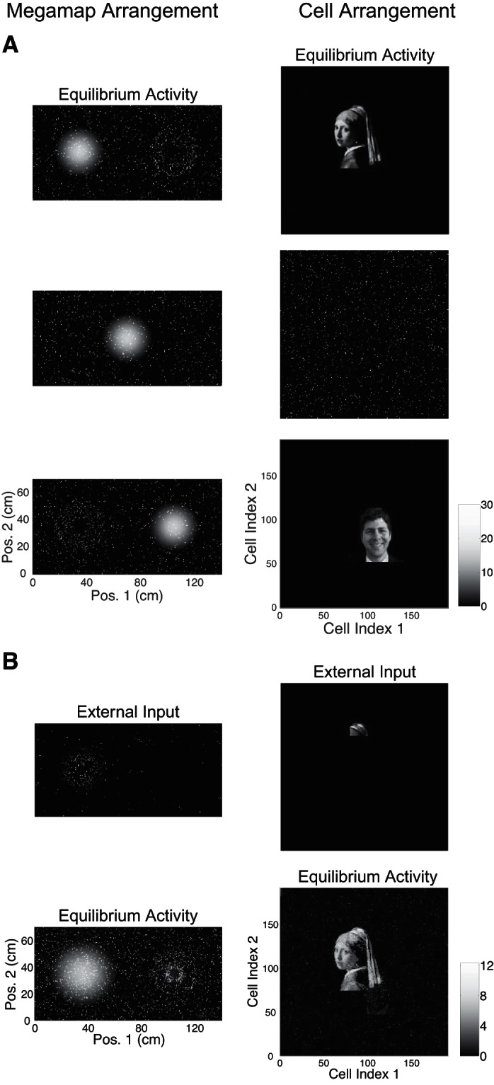
Dual interpretation of network activity patterns: example 2. A: the megamap represents a square region with 2 complex nonspatial patterns. When the animal is located at each of 3 locations, the equilibrium firing rates (Hz) are visualized in 2 ways (Fig. 13) to reveal the spatial (left) and nonspatial (right) information carried by the single network activity vector. The ghost effect in the megamap arrangement at locations corresponding to an image (top and bottom) is a result of the 16% of cells that represent both images. This overlap is much higher than the ∼6% of overlap between any other pair of activity bumps. As a result, the megamap has greater than average activity near the first image as a reflection of the robust activity bump near the second image, and vice versa. The multiplicity and randomness of the place code permit these 2 overlapping images to be embedded into the spatial framework of the megamap. B: the attractor network can perform pattern completion. Top, only cells representing the bun receive external input. Bottom, the equilibrium activity represents the complete learned pattern. The initial state is random. Supplemental Video S2 shows the 2 visualizations as the animal moves continuously across the region.

Suppose hippocampal pyramidal cells do not inherently encode either space or nonspatial objects, but rather can be responsive to both. Suppose further that a given salient nonspatial object is encoded through an arbitrary activity pattern across a subset of these cells. Through associative plasticity, cells encoding a nonspatial object should bind to place cells representing nearby locations, effectively forming place fields at the location of the object. In other subregions of the environment, these same cells may encode other objects or locations. A set of nonspatial patterns can then be seamlessly incorporated into the megamap by plotting the activity of each cell at each of its place field centers on the megamap (Fig. 1C), including the locations of the objects they encode.

One may visualize the resulting activity of the attractor network in two ways: by the megamap representation (Fig. 13A) or by resorting cells so that each cell's activity is plotted at a single preset pixel (Fig. 13B). As the animal traverses the environment, the former view shows the activity bump continuously encoding space, whereas the latter view of the same network activity shows the activation of discrete nonspatial memories (Figs. 14 and 15, Supplemental Videos S1 and S2). As expected of a discrete attractor, the megamap can perform pattern completion over these nonspatial memories whether operating in the WTA mode (Fig. 14B) or the combinatorial mode (Fig. 15B). This dual interpretation may potentially aid in developing unified theories of spatial and nonspatial memory to account for the “where” and “what” components of episodic memory.

Fig. 13.

Schematic for the visualization of spatial and nonspatial information encoded by a single network activity vector. In this schematic 36 place cells represent a 25 × 5-cm² region. A: for the megamap arrangement, each place cell is placed at each of its place field centers, as illustrated in Fig. 1C. The location of each cell in the megamap is indicated by the cell number, and cells 1–4 are additionally indicated by color. Cell 2 does not appear on the megamap because it has no place fields in the region. Pos., position. B: for the cell arrangement, each place cell is placed at a single preset pixel, regardless of its place fields. The 2 arrangements give 2 different ways to visualize the same network activity pattern. Unless the nonspatial activity patterns are orthogonal, this dual interpretation of the network activity requires place cells to have multiple, irregularly spaced place fields.

Nonspatial patterns can be bound to any attractor network representing space, but the dual representation is possible only if the nonspatial patterns are orthogonal or if place cells have the flexible representation of the megamap. In the nonorthogonal case, a cell participating in multiple nonspatial activity patterns must have place fields at the locations of each object it encodes. If the objects are placed randomly in the environment, the cell must have multiple, irregularly spaced place fields to incorporate the patterns into the cognitive map through the dual representation. Although one can model the associative binding of nonspatial patterns to the single-peaked attractor chart (Rolls et al. 2002), the spatial and nonspatial components of the environment would be encoded separately by two populations of cells, namely, by place cells and cells encoding objects.

Experimental predictions.

The megamap theory posits that hippocampal place cells are flexibly recombined to represent a large space through one seamless, stable cognitive map. Unlike the megamap, all other existing attractor models of place cells imply an exclusion principle. That is, there exists a neighborhood around each place field of a given cell in which the cell is excluded from having an additional place field. For example, a cell in the single-peaked chart (Fig. 1A) is excluded from exhibiting another place field anywhere in the region. Similarly, if the hippocampus were to partition an environment and represent each subregion by a different chart (Fig. 1B), then a cell with a place field in one subregion would be excluded from firing at any other location in the same subregion. Whereas all three models predict a localized activity bump over the animal's location, the single-peaked cognitive map is clean, the partitioned cognitive map restricts scattered activity to subregions that do not contain the activity bump, and activity is scattered throughout the megamap (Fig. 16A). The differing predictions of the three models could be tested through recordings in large two-dimensional environments, where the predicted scattered activity plotted redundantly at each cell's place field centers should be above the background noise.

A second distinguishing feature of the attractor models is the distance to nearest neighbor, or the distance from the center of a given place field to that of the closest place field of the same cell. Place fields that are close to their nearest neighbors should cluster near the artificial boundaries of a partitioned environment but should be evenly distributed throughout the megamap (Fig. 16B). If place fields in the megamap follow the Poisson distribution, then the distance to nearest neighbor follows the exponential distribution (Eq. 16) over a long, narrow track, which may be considered as approximately one-dimensional, and follows the Rayleigh distribution (Eq. 15) over a large two-dimensional environment (Figs. 2C and 16, C and D). Whereas the probability decays monotonically as the distance increases for the former case, the probability in a two-dimensional environment peaks at 1/$\sqrt{2\pi \lambda }$ ≈ 85 cm for λ = 0.22 m⁻². In either case, the distance to nearest neighbor over the megamap (but not over the partitioned environment) should be statistically unchanged whether the nearest neighbor is taken from place fields of the same cell or from place fields of any other single cell with the same average density of place fields (Fig. 16, C and D). With respect to these predictions, existing data are consistent with the megamap theory (see discussion).

The megamap shares several properties with the well-studied single-peaked attractor map of a small standard recording enclosure, including the relative stability of place fields in the CA3 compared with that of the CA1 (Lee et al. 2004; Vazdarjanova and Guzowski 2004), the persistence of place fields without external input (Figs. 6A and 7A; Quirk et al. 1990), and the sigmoidal relationship between changes in the spatial cues and changes in the CA3 representation (Guzowski et al. 2004; O'Reilly and McClelland 1994) due to pattern completion and pattern separation (Fig. 12). In addition, as the external input weakens, the amplitude of the activity bump should be largely maintained (Fig. 6), but it should slowly drift away from all but a relative few locations (Fig. 7). One must control the external input into the hippocampus to test these properties directly, perhaps by selective inactivation of the entorhinal cortex and current injection into subsets of hippocampal place cells.

The megamap provides a specific prediction for the functional connectome in the hippocampus. According to the standard theory, each place cell forms strong recurrent connections onto a single group of neighboring place cells on the chart. In contrast, a place cell with multiple place fields should form strong recurrent connections onto multiple groups of neighbors on the megamap (Fig. 5C). This could be a factor behind the variable spatial density of place fields found experimentally (Rich et al. 2014), because it implies that a cell with more place fields receives more recurrent excitation on average at a newly encountered location. As a by-product of the unique structure of its recurrent connections, the megamap may transition from the winner-take-all mode to the combinatorial mode as the learned environment becomes sufficiently large (Figs. 10 and 11). This transition should be accompanied by a loss of hysteresis (Fig. 11C) and weaker pattern separation while pattern completion remains strong (Fig. 11D and 12). These effects are potentially observable in experiments.

The flexibility of place cell recombinations also permits the megamap to incorporate nonspatial information through a novel dual interpretation (Figs. 14 and 15). Although the nonspatial patterns of these two examples are artificial, the dual interpretation may provide a useful visualization tool for testing hypotheses about the hippocampal representation of nonspatial information. A plausible alternative theory is that a continuous attractor network incorporates nonspatial information through associative binding of nonspatial cells to place cells (Rolls et al. 2002). A cell representing a nonspatial cue should not exhibit place fields in the region according to this theory, but it may have additional place fields elsewhere in the region according to the megamap theory. This prediction is experimentally testable.

DISCUSSION

We present an ideal model for a hippocampal attractor network that stabilizes the flexible representation of a large space. In addition to offering a concise description of the large cognitive map, the megamap has several unique properties that render it suitable as a basic building block for more comprehensive theories of hippocampal networks. The ideal megamap treats all spatial locations uniformly, providing one seamless cognitive map without any exclusion zones prohibiting place field multiplicity (Fig. 16). Its flexible representation also gives the megamap the potential to represent spaces of any size with a fixed spatial resolution (Figs. 3 and 4). Furthermore, the megamap is stable, because structured recurrent excitation always attracts the network activity to a localized activity bump bound to the animal's location by a relatively weak, noisy, or incomplete external input (Figs. 5–7 and 12). Finally, the megamap can be extended continuously (Figs. 8 and 9) and has emergent properties that permit it to adapt to environmental changes (Figs. 10–12) and incorporate nonspatial information (Figs. 14 and 15).

The concept of the megamap emerges naturally when one examines how hippocampal place fields are distributed in larger environments. Earlier experiments, confined to smaller chambers in which a place cell often shows no more than one place field (Muller 1996; O'Keefe and Nadel 1978) have understandably led to numerous attractor network models that are variants of the same basic motif: a rigid map in which each cell appears only once. These models naturally account for place field stability in a static environment (Quirk et al. 1990; Thompson and Best 1990) and coherence upon manipulation or removal of environmental cues, particularly in the CA3, presumably due to its recurrent connections (Harris et al. 2003; Johnston and Amaral 1998; Vazdarjanova and Guzowski 2004). However, models built on the framework of a single-peaked attractor network do not extend naturally to large environments (McNaughton et al. 2006). The idea of flexible cell recombinations on which the megamap is based (Fig. 1C) follows logically from the multiplicity and irregularity of place fields in large environments (Fenton et al. 2008; Maurer et al. 2006; Park et al. 2011; Rich et al. 2014) and the Hebbian-like associative plasticity observed in the hippocampus (Bliss and Collingridge 1993; McNaughton and Nadel 1990; Vazdarjanova and Guzowski 2004).

Although recent experimental studies have begun to quantify the multiplicity of place fields in large environments (Fenton et al. 2008; Maurer et al. 2006; Park et al. 2011; Rich et al. 2014), it has long been known that a minority of place cells exhibit multiple place fields in standard (<1 m²) recording enclosures (Muller 1996; O'Keefe and Nadel 1978). Accordingly, many previous modeling studies also allowed a place cell to have multiple place fields within small standard environments (Burgess 2007). For example, multiple place fields are expected if the given place cell relies on sensory inputs whose combined strength peaks at multiple spatial locations (Ji and Wilson 2007; Zipser 1985). More explicitly, multiple place fields have been generated in models by combining inputs from boundary vector cells in the subiculum, parasubiculum, and medial entorhinal cortex (Burgess et al. 2000; Hartley et al. 2000; Lever et al. 2009; O'Keefe and Burgess 1996); grid cells in the medial entorhinal cortex (Azizi et al. 2014; Fuhs and Touretzky 2006; Lyttle et al., 2013; McNaughton et al. 2006; Monaco and Abbott 2011; Savelli and Knierim 2010); and granule cells in the dentate gyrus (Cerasti and Treves 2010). A minority of cells have also been shown to exhibit multiple place fields in attractor network models generated from the multichart architecture (Samsonovich and McNaughton 1997; see Fig. 1B) or from an unsupervised learning process (Cerasti and Treves 2013; Kali and Dayan 2000). The megamap provides a theoretical framework on which attractor networks such as these could be extended to cover a large space by formalizing the ideal attractor network representing a large environment through one seamless cognitive map. Although additional biological mechanisms could always be incorporated into the model, the megamap is the simplest implementation for which the flexible representation of a large space is compatible with the stability of attractor dynamics.

Capacity of the megamap.

The flexible representation of place cells gives the megamap the potential to represent huge areas, but the megamap's capacity is limited by the number of activity bump locations that can be accurately learned by the attractor network (Figs. 8 and 9). Although we leave a detailed study of the capacity for future work, in this report we provide a rough heuristic scaling argument for the megamap's capacity.

It is well established that the number of distinct memory patterns that can be stored in a Hopfield-type network grows linearly with N, the number of cells (Amit 1989; Hopfield 1984). Similarly, the number of charts stored in the multichart model grows linearly with N (Battaglia and Treves 1998; Samsonovich and McNaughton 1997). It has also been shown that the capacity is limited by the number of connections per cell (Roudi and Latham 2007), but this should not be a limiting factor in the rat CA3 with 10⁵ cells since a given pyramidal cell has roughly 10⁴ recurrent connections (Johnston and Amaral 1998). Hence, we ignore this factor below.

The capacity is also affected by the place field width, σ_u, which varies in the hippocampus from roughly 0.1 to 10 m (Kjelstrup et al. 2008), and the place field density, λ. Using dimensional analysis (Barenblatt 1996), we propose that the capacity (area covered by the megamap) scales as

$$A\hspace{0.17em}\mathrm{\propto }\hspace{0.17em}N{\mathrm{\sigma }}_u^{\mathrm{\alpha }}{\mathrm{\lambda }}^{\mathrm{\beta }}$$ (21)

for some constants α and β. If we coarsen the spatial representation by hypothetically increasing the unit length, λ should scale with σ_u⁻² without affecting the network dynamics. Replacing λ with σ_u⁻² and matching dimensions in Eq. 21, we obtain

$$A\hspace{0.17em}\mathrm{\propto }\hspace{0.17em}N{\mathrm{\sigma }}_u^{\mathrm{2}}\mathrm{.}$$

In our simulations, we found that the megamap accurately represents about 100 m² when N ≈ 10⁴ cells and σ_u ≈ 0.1 m (Fig. 9). Hence, we estimate that a megamap with N ≈ 10⁵ cells and σ_u = 0.1 m should accurately represent about 1,000 m². This capacity is likely more than sufficient for covering the typical natural habitats of rats. Tracking experiments show that in the wild, a rat often travels many hundreds of meters along a primarily narrow passage, and so the total foraging area is typically far below 1,000 m² (Davis 1953; Innes and Skipworth 1983; Lambert et al. 2008; Taylor 1978;).

Finally, larger place fields may greatly increase the megamap coverage area. Assuming 1% of place cells (N = 10³) have the place field width σ_u = 10 m, then A = 10⁵ m², which could cover a 10-km × 10-m route. Of course, the spatial resolution of such a megamap would be much worse due to the smaller place field density (Eq. 4). In reality, the hippocampus likely binds together megamaps of varying scale for a coarse representation of long distances and a fine representation of subregions of interest, such as feeding sites.

Poisson distribution of place fields.

Cellular mechanisms underlying the recruitment of place cells in new territories may include the preexisting structure of recurrent connections (Dragoi and Tonegawa 2011), the excitability of place cells (Lee et al. 2012), a pattern separation process in the dentate gyrus (Aimone et al. 2011; Cerasti and Treves 2010; Leutgeb et al. 2007), and NMDA-dependent synaptic plasticity (Nakazawa et al. 2004), perhaps enhanced by acetylcholine (Hasselmo 2006). The megamap could be extended to incorporate these biological mechanisms without affecting the qualitative results.

The megamap is the most flexible when the place fields of each cell obey independent Poisson processes. The Poisson distribution of place fields approximates experimental data from a moderately large open-field environment (Fig. 2, Table 1). However, the Poisson distribution underestimates the number of cells with a relative large number of place fields, as shown by the prolonged tail in Fig. 2B. One can adapt the megamap to incorporate a variable place field density so that a minority of cells remain silent or have a relatively high propensity for exhibiting place fields. This modification is consistent with the data recorded over long tracks, for which place fields of individual cells follow the Poisson distribution with a variable field density among cells (Rich et al. 2014). It might also account for the exponential distribution of place fields across the population previously reported for long tracks (Maurer et al. 2006). As predicted by the megamap, the distance to nearest neighbor appears to follow the exponential distribution over a long track (Rich et al. 2014), to follow the Rayleigh distribution over a two-dimensional environment (Fig. 2C), and to show no clustering (Fenton et al. 2008; Park et al. 2011). Although the hippocampal representation of large open-field environments (>3 m²) is unknown, the hippocampus has been shown to uniquely represent several small open-field environments through global remapping among place cell ensembles in the CA3 (Alme et al. 2014). The representations appear to be independent except for a small minority of cells that fire in all environments. These results may point to a large hippocampal capacity, consistent with the megamap theory.

Union of stability and flexibility.

Stability and flexibility are two desirable properties of any hippocampal network model, but they naturally counteract one another. Although the activity bump drifts away from all but a discrete set of locations on the isolated megamap, relatively weak external input couples with strong, structured recurrent excitation to compensate for this loss of stability when the spatial representation is maximally flexible (Fig. 7). The megamap could be driven by more realistic external input than presented here. For example, place cells could track a weak path integration signal from grid cells innervating their distal dendrites (McNaughton et al. 2006). Similarly, a noisy signal for external landmarks carried by afferents in the lateral entorhinal cortex (Deshmukh and Knierim 2011; Knierim 2006; Knierim et al. 2014) could be sufficient for initial localization or error correction on the megamap.

Flexibility in the spatial representation leads to flexibility in the attractor map, permitting the megamap to stably combine embedded activity bumps. The combinatorial mode (Figs. 10 and 11) could lead to new associations or even permit partial remapping (Colgin et al. 2008; Jeffery 2011) if multiple megamaps were to represent distinct subsets of cues, as was shown for single-peaked attractor maps (Stringer et al. 2004). It also allows the activity pattern to gradually transition from one embedded attractor state to another (Fig. 11D), raising the possibility of an alternative explanation for the intermediate activity patterns found experimentally (Colgin et al. 2010; Leutgeb et al. 2005) to those offered by recent modeling studies (Rennó-Costa et al. 2014; Solstad et al. 2014). On a higher level, the combinatorial mode is conducive for combining memories never encountered together to simulate possible future episodes, an ability shown to rely on the same circuits critical for episodic memory in humans (Schacter and Addis 2007). Although other attractor models have modified the dynamical system to sustain multiple activity bumps (Moldakarimov et al. 2005; Samsonovich 1998; Stringer et al. 2004), the combinatorial mode emerges spontaneously in a sufficiently large megamap.

Union of spatial and nonspatial representations.

The megamap is locally continuous in the sense that the patterns of active cells representing two nearby locations are similar, but the patterns become uncorrelated as the distance exceeds the place field size. Uncorrelated activity patterns, like the discrete set of patterns stored in a Hopfield network (Hopfield 1982), may encode information about an environment in addition to the animal's spatial position. The megamap can store any nonspatial pattern if its active cells have place fields at the corresponding location. This should occur naturally through associative plasticity, because cells representing a salient nonspatial cue should be co-active with place cells representing nearby locations.

It has been suggested that hippocampal networks may encode discrete attractors encoding nonspatial information, whereas the continuous attractor dynamics apparent in place cell activity may be a mere reflection of the dynamics in the upstream grid cell network (Jeffery 2011; Knierim and Zhang 2012). We propose that the hippocampal attractor network can be considered both continuous and discrete, depending on one's point of view. The megamap arrangement reveals a quasi-continuous attractor map encoding space, whereas the cell arrangement of the same activity patterns reveals a discrete set of nonspatial memories. This novel perspective offered by the dual interpretation unites spatial and nonspatial representations under a single principle of flexible cell recombinations.

The megamap is the first attractor model for which the dual interpretation (Figs. 13–15) is possible. In models nonspatial memories are typically represented by random recombinations of cells (Hopfield 1982), just as the megamap represents distinct locations through random recombinations of place cells. Since the cues may be placed anywhere in the region, a cell representing multiple cues must have multiple, irregularly spaced place fields according to the dual interpretation. Similarly, there should be no correlation among place field pairs. These two requirements are the exact properties of the megamap that distinguish it from standard attractor models of place cell networks. Although previous models have shown how an autoassociative network may bind spatial and nonspatial information (Rolls et al. 2002), the dual interpretation is not possible for these models unless the nonspatial patterns are orthogonal. The megamap can incorporate any activity pattern, even complex visual patterns such as faces (Fig. 15), as long as distinct patterns correspond to well-separated locations in the environment.

Megamap as a building block.

The megamap can be used to construct more general theories in the same way as the single-peaked attractor map (chart) has been used. Although we have focused on a single megamap here, it is straightforward to embed multiple megamaps in the same network. For example, a single network may store multiple megamaps representing multiple environments (Samsonovich and McNaughton 1997) or distinct subsets of cues in the same environment (Stringer et al. 2004), permitting global and partial remapping, respectively. Similarly, the megamap may encode context through a variable firing rate (Solstad et al. 2014), permitting rate remapping. Megamaps with different scales (Kjelstrup et al. 2008) could be coupled together for a coarse representation of long distances and fine representations of subregions of interest, such as feeding sites. Since the animal's path between feeding sites is likely long and narrow, the learning procedure of the model may need to be adapted in this case to incorporate known spatial properties in a one-dimensional environment, such as the directionality of place fields (Muller et al. 1994). Using the megamap as the building block for these models instead of a single-peaked continuous attractor map eliminates the size limitations and provides the flexibility to adapt to environmental changes and to naturally incorporate nonspatial information.

GRANTS

This work is funded by Air Force Office of Scientific Research Grant FA9550-12-1-0018 and National Institute of Mental Health Grant R01MH079511.

DISCLOSURES

No conflicts of interest, financial or otherwise, are declared by the authors.

AUTHOR CONTRIBUTIONS

K.R.H. and K.Z. conception and design of research; K.R.H. performed experiments; K.R.H. analyzed data; K.R.H. and K.Z. interpreted results of experiments; K.R.H. prepared figures; K.R.H. drafted manuscript; K.R.H. and K.Z. edited and revised manuscript; K.R.H. and K.Z. approved final version of manuscript.

REFERENCES

- Abbott L, Nelson S. Synaptic plasticity: taming the beast. Nat Neurosci 3: 1178–1183, 2000. [DOI] [PubMed] [Google Scholar]
- Aimone J, Deng W, Gage F. Resolving new memories: a critical look at the dentate gyrus, adult neurogenesis, and pattern separation. Neuron 70: 589–596, 2011. [DOI] [PMC free article] [PubMed] [Google Scholar]
- Alme C, Miao C, Jezek K, Treves A, Moser E, Moser M. Place cells in the hippocampus: eleven maps for eleven rooms. Proc Natl Acad Sci USA 111: 18428–18435, 2014. [DOI] [PMC free article] [PubMed] [Google Scholar]
- Amit D. Modeling Brain Function: the World of Attractor Neural Networks. Cambridge, UK: Cambridge University Press, 1989. [Google Scholar]
- Azizi A, Schieferstein N, Cheng S. The transformation from grid cells to place cells is robust to noise in the grid pattern. Hippocampus 24: 912–919, 2014. [DOI] [PubMed] [Google Scholar]
- Barenblatt GI. Scaling, Self-similarity, and Intermediate Asymptotics. Cambridge, UK: University Press, 1996. [Google Scholar]
- Battaglia F, Treves A. Attractor neural networks storing multiple space representations: a model for hippocampal place fields. Phys Rev E 58: 7738–7753, 1998. [Google Scholar]
- Bliss T, Collingridge G. A synaptic model of memory: long-term potentiation in the hippocampus. Nature 361: 31–39, 1998. [DOI] [PubMed] [Google Scholar]
- Brown EN, Frank LM, Tang D, Quirk MC, Wilson MA. A statistical paradigm for neural spike train decoding applied to position prediction from ensemble firing patterns of rat hippocampal place cells. J Neurosci 18: 7411–7425, 1998. [DOI] [PMC free article] [PubMed] [Google Scholar]
- Burgess N. Computational models of the spatial and mnemonic functions of the hippocampus. In: The Hippocampus Book, edited by Andersen P, Morris R, Amaral D, Bliss T, and O'Keefe J. New York: Oxford University Press, 2007, p. 715–749. [Google Scholar]
- Burgess N, Jackson A, Hartley T, O'Keefe J. Predictions derived from modelling the hippocampal role in navigation. Biol Cybern 83: 301–312, 2000. [DOI] [PubMed] [Google Scholar]
- Cerasti E, Treves A. How informative are spatial CA3 representations established by the dentate gyrus? PLoS Comput Biol 6: e1000759, 2010. [DOI] [PMC free article] [PubMed] [Google Scholar]
- Cerasti E, Treves A. The spatial representations acquired in CA3 by self-organizing recurrent connections. Front Cell Neurosci 7: 112, 2013. [DOI] [PMC free article] [PubMed] [Google Scholar]
- Colgin L, Leutgeb S, Jezek K, Leutgeb J, Moser E, McNaughton B, Moser M. Attractor-map versus autoassociation based attractor dynamics in the hippocampal network. J Neurophysiol 104: 35–50, 2010. [DOI] [PMC free article] [PubMed] [Google Scholar]
- Colgin L, Moser E, Moser M. Understanding memory through hippocampal remapping. Trends Neurosci 31: 469–477, 2008. [DOI] [PubMed] [Google Scholar]
- Davidson TJ, Kloosterman F, Wilson MA. Hippocampal replay of extended experience. Neuron 63: 497–507, 2009. [DOI] [PMC free article] [PubMed] [Google Scholar]
- Davis D. The characteristics of rat populations. Q Rev Biol 28: 373–401, 1953. [DOI] [PubMed] [Google Scholar]
- Deshmukh S, Knierim J. Representation of non-spatial and spatial information in the lateral entorhinal cortex. Front Behav Neurosci 5: 69, 2011. [DOI] [PMC free article] [PubMed] [Google Scholar]
- Doboli S, Minai A, Best P. Latent attractors: a model for context-dependent place representations in the hippocampus. Neural Comput 12: 1009–1043, 2000. [DOI] [PubMed] [Google Scholar]
- Dragoi G, Tonegawa S. Preplay of future place cell sequences by hippocampal cellular assemblies. Nature 469: 397–401, 2011. [DOI] [PMC free article] [PubMed] [Google Scholar]
- Egorov A, Hamam B, Fransen E, Hasselmo M, Alonso A. Graded persistent activity in entorhinal cortex neurons. Nature 420: 173–178, 2002. [DOI] [PubMed] [Google Scholar]
- Ermentrout G, Terman D. Mathematical Foundations of Neuroscience. New York: Springer, 2010. [Google Scholar]
- Fenton A, Kao HY, Neymotin S, Olypher A, Vayntrub Y, Lytton W, Ludvig N. Unmasking the CA1 ensemble place code by exposures to small and large environments: more place cells and multiple, irregularly arranged, and expanded place fields in the larger space. J Neurosci 28: 11250–11262, 2008. [DOI] [PMC free article] [PubMed] [Google Scholar]
- Fiete I, Burak Y, Brookings T. What grid cells convey about rat location. J Neurosci 28: 6858–6871, 2008. [DOI] [PMC free article] [PubMed] [Google Scholar]
- Fortin N, Agster K, Eichenbaum H. Critical role of the hippocampus in memory for sequences of events. Nat Neurosci 5: 458–462, 2002. [DOI] [PMC free article] [PubMed] [Google Scholar]
- Fuhs M, Touretzky D. A spin glass model of path integration in rat medial entorhinal cortex. J Neurosci 26: 4266–4276, 2006. [DOI] [PMC free article] [PubMed] [Google Scholar]
- Guzowski J, Knierim J, Moser E. Ensemble dynamics of hippocampal regions CA3 and CA1. Neuron 44: 581–584, 2004. [DOI] [PubMed] [Google Scholar]
- Guzowski J, McNaughton B, Barnes C, Worley P. Environment-specific expression of the immediate-early gene Arc in hippocampal neuronal ensembles. Nat Neurosci 2: 1120–1124, 1999. [DOI] [PubMed] [Google Scholar]
- Harris K, Csicsvari J, Hirase H, Dragoi G, Buzsák G. Organization of cell assemblies in the hippocampus. Nature 424: 552–556, 2003. [DOI] [PubMed] [Google Scholar]
- Hartley T, Burgess N, Leve C, Cacucci F, O'Keefe J. Modeling place fields in terms of the cortical inputs to the hippocampus. Hippocampus 10: 369–379, 2000. [DOI] [PubMed] [Google Scholar]
- Hasselmo M. The role of acetylcholine in learning and memory. Curr Opin Neurobiol 16: 710–715, 2006. [DOI] [PMC free article] [PubMed] [Google Scholar]
- Hines M. Efficient computation of branched nerve equations. Int J Biomed Comput 15: 69–76, 1984. [DOI] [PubMed] [Google Scholar]
- Hopfield J. Neural networks and physical systems with emergent collective computational abilities. Proc Natl Acad Sci USA 79: 2554–2558, 1982. [DOI] [PMC free article] [PubMed] [Google Scholar]
- Hopfield J. Neurons with graded response have collective computational properties like those of two-state neurons. Proc Natl Acad Sci USA 81: 3088–3092, 1984. [DOI] [PMC free article] [PubMed] [Google Scholar]
- Innes J, Skipworth J. Home ranges of ship rats in a small New Zealand forest as revealed by trapping and tracking. NZ J Zool 10: 99–110, 1983. [Google Scholar]
- Ivancevic V, Ivancevic T. High-Dimensional Chaotic and Attractor Systems: a Comprehensive Introduction. Dordrecht, The Netherlands: Springer, 2007. [Google Scholar]
- Jazayeri M, Movshon J. Optimal representation of sensory information by neural populations. Nat Neurosci 9: 690–696, 2006. [DOI] [PubMed] [Google Scholar]
- Jeffery K. Place cells, grid cells, attractors, remapping. Neural Plast 2011: 182602. 2011. [DOI] [PMC free article] [PubMed] [Google Scholar]
- Ji D, Wilson M. Coordinated memory replay in the visual cortex and hippocampus during sleep. Nat Neurosci 10: 100–107, 2007. [DOI] [PubMed] [Google Scholar]
- Jochems A, Yoshida M. Persistent firing supported by an intrinsic cellular mechanism in hippocampal CA3 pyramidal cells. Eur J Neurosci 38: 2250–2259, 2013. [DOI] [PubMed] [Google Scholar]
- Johnston D, Amaral D. Hippocampus. In: The Synaptic Organization of the Brain, edited by Shepherd G. New York: Oxford University Press, 1998, chapt. 10, p. 417–458. [Google Scholar]
- Kali S, Dayan P. The involvement of recurrent connections in area CA3 in establishing the properties of place fields: a model. J Neurosci 20: 7463–7477, 2000. [DOI] [PMC free article] [PubMed] [Google Scholar]
- Kay S. Fundamentals of Statistical Signal Processing: Estimation Theory. Upper Saddle River, NJ: Prentice Hall, 1993. [Google Scholar]
- Kjelstrup K, Solstad T, Brun V, Hafting T, Leutgeb S, Witter M, Moser E, Moser M. Finite scale of spatial representation in the hippocampus. Science 321: 140–143, 2008. [DOI] [PubMed] [Google Scholar]
- Knierim J. Hippocampal place cells: parallel input streams, subregional processing, and implications for episodic memory. Hippocampus 16: 755–764, 2006. [DOI] [PubMed] [Google Scholar]
- Knierim J, Neunuebel J, Deshmukh S. Functional correlates of the lateral and medial entorhinal cortex: objects, path integration and local-global reference frames. Philos Trans R Soc Lond B Biol Sci 369: 20130369, 2013. [DOI] [PMC free article] [PubMed] [Google Scholar]
- Knierim J, Zhang K. Attractor dynamics of spatially correlated neural activity in the limbic system. Annu Rev Neurosci 35: 267–286, 2012. [DOI] [PMC free article] [PubMed] [Google Scholar]
- Kubie J, Muller R, Bostock E. Spatial firing properties of hippocampal theta cells. J Neurosci 10: 1110–1123, 1990. [DOI] [PMC free article] [PubMed] [Google Scholar]
- Kulkarni M, Zhang K, Kirkwood A. Single-cell persistent activity in anterodorsal thalamus. Neurosci Lett 498: 179–184, 2011. [DOI] [PMC free article] [PubMed] [Google Scholar]
- Lambert M, Quy R, Smith R, Cowan D. The effect of habitat management of home-range size and survival of rural Norway rat populations. J Appl Ecol 45: 1753–1761, 2008. [Google Scholar]
- Lee D, Lin B, Lee A. Hippocampal place fields emerge upon single-cell manipulation of excitability during behavior. Science 337: 849–853, 2012. [DOI] [PubMed] [Google Scholar]
- Lee I, Yoganarashimha D, Rao G, Knierim J. Comparison of population coherence of place cells in hippocampal subfields CA1 and CA3. Nature 430: 456–459, 2004. [DOI] [PubMed] [Google Scholar]
- Leutgeb J, Leutgeb S, Moser M, Moser E. Pattern separation in the dentate gyrus and CA3 of the hippocampus. Science 315: 961–966, 2007. [DOI] [PubMed] [Google Scholar]
- Leutgeb J, Leutgeb S, Treves A, Meyer R, Barnes C, McNaughton B, Moser M, Moser E. Progressive transformation of hippocampal neuronal representations in “morphed” environments. Neuron 48: 345–358, 2005. [DOI] [PubMed] [Google Scholar]
- Leutgeb S, Leutgeb J. Pattern separation, pattern completion, and new neuronal codes within a continuous CA3 map. Learn Mem 14: 745–757, 2007. [DOI] [PubMed] [Google Scholar]
- Lever C, Burton S, Jeewajee A, O'Keefe J, Burgess N. Boundary vector cells in the subiculum of the hippocampal formation. J Neurosci 29: 9771–9777, 2009. [DOI] [PMC free article] [PubMed] [Google Scholar]
- Li Z, Dayan P. Computational differences between asymmetrical and symmetrical networks. Network 10: 59–77, 1999. [PubMed] [Google Scholar]
- Lyttle D, Gereke B, Lin K, Fellous J. Spatial scale and place field stability in a grid-to-place cell model of the dorsoventral axis of the hippocampus. Hippocampus 23: 729–744, 2013. [DOI] [PMC free article] [PubMed] [Google Scholar]
- Marr D. Simple memory: a theory for archicortex. Philos Trans R Soc Lond B Biol Sci 262: 23–81, 1971. [DOI] [PubMed] [Google Scholar]
- Mathis A, Herz A, Stemmler M. Optimal population codes for space: grid cells outperform place cells. Neural Comput 24: 2280–2317, 2012. [DOI] [PubMed] [Google Scholar]
- Maurer A, Cowen S, Burke S, Barnes C, McNaughton B. Organization of hippocampal cell assemblies based on theta phase precession. Hippocampus 16: 785–794, 2006. [DOI] [PubMed] [Google Scholar]
- McNaughton B, Battaglia F, Jensen O, Moser E, Moser M. Path integration and the neural basis of the ‘cognitive map’. Nat Rev Neurosci 7: 663–678, 2006. [DOI] [PubMed] [Google Scholar]
- McNaughton B, Nadel L. Hebb-Marr networks and the neurobiological representation of action in space. In: Neuroscience and Connectionist Theory, edited by Gluck M, Rumelhart D. Hillsdale, NJ: Lawrence Erlbaum, 1990, chapt, 1, p. 1–63. [Google Scholar]
- Moldakarimov S, Rollenhagen J, Olson C, Chow C. Competitive dynamics in cortical responses to visual stimuli. J Neurophysiol 94: 3388–3396, 2005. [DOI] [PubMed] [Google Scholar]
- Monaco J, Abbott L. Modular realignment of entorhinal grid cell activity as a basis for hippocampal remapping. J Neurosci 31: 9414–9425, 2011. [DOI] [PMC free article] [PubMed] [Google Scholar]
- Muller R. A quarter of a century of place cells. Neuron 17: 979–990, 1996. [DOI] [PubMed] [Google Scholar]
- Muller R, Bostock E, Taube J, Kubie J. On the directional firing properties of hippocampal place cells. J Neurosci 14: 7235–7251, 1994. [DOI] [PMC free article] [PubMed] [Google Scholar]
- Muller R, Kubie J, Ranck J Jr.. Spatial firing patterns of hippocampal complex-spike cells in a fixed environment. J Neurosci 7: 1935–1950, 1987. [DOI] [PMC free article] [PubMed] [Google Scholar]
- Nakazawa K, McHugh T, Wilson M, Tonegawa S. NMDA receptors, place cells and hippocampal spatial memory. Nat Rev Neurosci 5: 361–372, 2004. [DOI] [PubMed] [Google Scholar]
- Neunuebel J, Knierim J. CA3 retrieves coherent representations from degraded input: direct evidence for CA3 pattern completion and dentate gyrus pattern separation. Nature 81: 416–427, 2014. [DOI] [PMC free article] [PubMed] [Google Scholar]
- O'Keefe J. Hippocampal neurophysiology in the behaving animal. In: The Hippocampus Book, edited by Andersen P, Morris R, Amaral D, Bliss T, O'Keefe J. New York: Oxford University Press,2007, chapt. 11, p. 523–534. [Google Scholar]
- O'Keefe J, Burgess N. Geometric determinants of the place fields of hippocampal neurons. Nature 381: 425–428, 1996. [DOI] [PubMed] [Google Scholar]
- O'Keefe J, Nadel L. The Hippocampus as a Cognitive Map. Oxford, UK: Clarendon, 1978. [Google Scholar]
- O'Reilly R, McClelland J. Hippocampal conjunctive encoding, storage, and recall: avoiding a trade-off. Hippocampus 4: 661–682, 1994. [DOI] [PubMed] [Google Scholar]
- Park E, Dvorak D, Fenton A. Ensemble place codes in hippocampus: CA1, CA3, and dentate gyrus place cells have multiple place fields in large environments. PLoS One 6: e22349, 2011. [DOI] [PMC free article] [PubMed] [Google Scholar]
- Peyrache A, Lacroix M, Petersen P, Buzsáki G. Internally organized mechanisms of the head direction sense. Nat Neurosci 18: 569–575, 2015. [DOI] [PMC free article] [PubMed] [Google Scholar]
- Pouget A, Zhang K, Deneve S, Latham P. Statistically efficient estimation using population coding. Neural Comput 10: 373–401, 1998. [DOI] [PubMed] [Google Scholar]
- Quirk G, Muller R, Kubie J. The firing of hippocampal place cells in the dark depends on the rat's recent experience. J Neurosci 10: 2008–2017, 1990. [DOI] [PMC free article] [PubMed] [Google Scholar]
- Redish A, Elga A, Touretzky D. A coupled attractor model of the rodent head direction system. Network 7: 671–685, 1996. [Google Scholar]
- Renart A, Song P, Wang X. Robust spatial working memory through homeostatic synaptic scaling in heterogeneous cortical networks. Neuron 38: 473–485, 2003. [DOI] [PubMed] [Google Scholar]
- Rennó-Costa C, Lisman J, Verschure P. A signature of attractor dynamics in the CA3 region of the hippocampus. PLoS Comput Biol 10: e1003641, 2014. [DOI] [PMC free article] [PubMed] [Google Scholar]
- Rich P, Liaw H, Lee A. Large environments reveal the statistical structure governing hippocampal representations. Science 345: 814–817, 2014. [DOI] [PubMed] [Google Scholar]
- Rolls E. An attractor network in the hippocampus: theory and neurophysiology. Learn Mem 14: 714–731, 2007. [DOI] [PubMed] [Google Scholar]
- Rolls E, Stringer S, Trappenberg T. A unified model of spatial and episodic memory. Proc Biol Sci 269: 1087–1093, 2002. [DOI] [PMC free article] [PubMed] [Google Scholar]
- Rolls E, Treves A, Tovee M. The representational capacity of the distributed encoding of information provided by populations of neurons in primate temporal visual cortex. Exp Brain Res 114: 149–162, 1997. [DOI] [PubMed] [Google Scholar]
- Roudi Y, Latham PE. A balanced memory network. PLoS Comput Biol 3: e141, 2007. [DOI] [PMC free article] [PubMed] [Google Scholar]
- Samsonovich A. Hierarchical multichart model of the hippocampal cognitive map. In: Proceedings of the 5th Joint Symposium on Neural Computation, University of California, San Diego, 1998, p. 140–147. [Google Scholar]
- Samsonovich A, McNaughton B. Path integration and cognitive mapping in a continuous attractor neural network model. J Neurosci 17: 5900–5920, 1997. [DOI] [PMC free article] [PubMed] [Google Scholar]
- Savelli F, Knierim J. Hebbian analysis of the transformation of medial entorhinal grid-cell inputs to hippocampal place fields. J Neurophysiol 103: 3167–3183, 2010. [DOI] [PMC free article] [PubMed] [Google Scholar]
- Schacter D, Addis D. The cognitive neuroscience of constructive memory: remembering the past and imagining the future. Philos Trans R Soc Lond B Biol Sci 362: 773–786, 2007. [DOI] [PMC free article] [PubMed] [Google Scholar]
- Seelig J, Jayaraman V. Neural dynamics for landmark orientation and angular path integration. Nature 521: 186–191, 2015. [DOI] [PMC free article] [PubMed] [Google Scholar]
- Skaggs W, Knierim J, Kudrimoti H, McNaughton B. A model of the neural basis of the rat's sense of direction. Adv Neural Inf Process Syst 7: 173–180, 1995. [PubMed] [Google Scholar]
- Solstad T, Yousif H, Sejnowski T. Place cell rate remapping by CA3 recurrent collaterals. PLoS Comput Biol 10: e1003648, 2014. [DOI] [PMC free article] [PubMed] [Google Scholar]
- Stella F, Cerasti E, Si B, Jezek K, Treves A. Self-organization of multiple spatial and context memories in the hippocampus. Neurosci Biobehav Rev 36: 1609–1625, 2012. [DOI] [PubMed] [Google Scholar]
- Stensola H, Stensola T, Solstad T, Frøland K, Moser M, Moser E. The entorhinal grid map is discretized. Nature 492: 72–78, 2012. [DOI] [PubMed] [Google Scholar]
- Stringer S, Rolls E, Trappenberg T. Self-organising continuous attractor networks with multiple activity packets, and the representation of space. Neural Netw 17: 5–27, 2004. [DOI] [PubMed] [Google Scholar]
- Stringer S, Rolls E, Trappenberg T, de Araujo I. Self-organizing continuous attractor networks and path integration: two-dimensional models of place cells. Network 13: 429–446, 2002. [PubMed] [Google Scholar]
- Strogatz S. Nonlinear Dynamics and Chaos. Reading, MA: Addison-Wesley, 1994. [Google Scholar]
- Taylor K. Range of movement and activity of common rats (Rattus norvegicus) on agricultural land. J Appl Ecol 15: 663–677, 1978. [Google Scholar]
- Thompson L, Best P. Long-term stability of the place-field activity of single units recorded from the dorsal hippocampus of freely behaving rats. Brain Res 509: 299–308, 1990. [DOI] [PubMed] [Google Scholar]
- Tsodyks M. Attractor neural network models of spatial maps in hippocampus. Hippocampus 9: 481–489, 1999. [DOI] [PubMed] [Google Scholar]
- Vazdarjanova A, Guzowski J. Differences in hippocampal neuronal population responses to modifications of an environmental context: evidence for distinct, yet complementary, functions of CA3 and CA1 ensembles. J Neurosci 24: 6489–6496, 2004. [DOI] [PMC free article] [PubMed] [Google Scholar]
- Vogels T, Sprekeler H, Zene F, Clopath C, Gerstner W. Inhibitory plasticity balances excitation and inhibition in sensory pathways and memory networks. Science 334: 1569–1573, 2011. [DOI] [PubMed] [Google Scholar]
- Wilson H, Cowan J. Excitatory and inhibitory interactions in localized populations of model neurons. Biophys J 12: 1–24, 1972. [DOI] [PMC free article] [PubMed] [Google Scholar]
- Wilson M, McNaughton B. Dynamics of the hippocampal ensemble code for space. Science 261: 1055–1058, 1993. [DOI] [PubMed] [Google Scholar]
- Winograd M, Destexhe A, Sanchez-Vives M. Hyperpolarization-activated graded persistent activity in the prefrontal cortex. Proc Natl Acad Sci USA 105: 7298–7303, 2008. [DOI] [PMC free article] [PubMed] [Google Scholar]
- Wu S, Hamaguchi K, Amari S. Dynamics and computation of continuous attractors. Neural Comput 20: 994–1025, 2008. [DOI] [PubMed] [Google Scholar]
- Yoon K, Buice M, Barry C, Hayman R, Burgess N, Fiete I. Specific evidence of low-dimensional continuous attractor dynamics in grid cells. Nat Neurosci 16: 1077–1084, 2013. [DOI] [PMC free article] [PubMed] [Google Scholar]
- Yoshida M, Hasselmo M. Persistent firing supported by an intrinsic cellular mechanism in a component of the head direction system. J Neurosci 29: 4945–4952, 2009. [DOI] [PMC free article] [PubMed] [Google Scholar]
- Zhang K. Representation of spatial orientation by the intrinsic dynamics of the head-direction cell ensemble: a theory. J Neurosci 16: 2112–2126, 1996. [DOI] [PMC free article] [PubMed] [Google Scholar]
- Zhang K, Ginzburg I, McNaughton BL, Sejnowski TJ. Interpreting neuronal population activity by reconstruction: unified framework with application to hippocampal place cells. J Neurophysiol 79: 1017–1044, 1998. [DOI] [PubMed] [Google Scholar]
- Zipser D. A computational model of hippocampal place fields. Behav Neurosci 99: 1006–1018, 1985. [DOI] [PubMed] [Google Scholar]
Associated Data
This section collects any data citations, data availability statements, or supplementary materials included in this article.