COMPREHENSIVE CLASSIFICATION OF RETINAL BIPOLAR NEURONS BY SINGLE-CELL TRANSCRIPTOMICS

SUMMARY

Patterns of gene expression can be used to characterize and classify neuronal types. It is challenging, however, to generate taxonomies that fulfill the essential criteria of being comprehensive, harmonizing with conventional classification schemes, and lacking superfluous subdivisions of genuine types. To address these challenges, we used massively parallel single-cell RNA profiling and optimized computational methods on a heterogeneous class of neurons, mouse retinal bipolar cells (BCs). From a population of ~25,000 BCs we derived a molecular classification that identified 15 types including all types observed previously, and two novel types, one of which has a non-canonical morphology and position. We validated the classification scheme and identified dozens of novel markers using methods that match molecular expression to cell morphology. This work provides a systematic methodology for achieving comprehensive molecular classification of neurons, identifies novel neuronal types, and uncovers transcriptional differences that distinguish types within a class.

eTOC

Single-cell transcriptome sequencing of retinal bipolar cells reveals known and new types including one with a non-canonical morphology.

INTRODUCTION

Investigations into brain development, function, and disease depend upon accurate identification and categorization of cell types. Assignment of roles, genes, or pathologies to specific types allows fundamental processes to be understood with greater precision than when assigned to brain regions or broad classes of cells. Moreover, molecular identifiers of specific types enable comparison of results obtained at different times, in different laboratories, or following experimental perturbations. In model organisms, they enable genetic access, allowing neurons to be marked and manipulated. Accordingly, numerous methods have been developed to classify neurons (Seung and Sumbul, 2014).

Despite methodological advances, the enterprise of cell type categorization remains challenging for both technical and conceptual reasons. Conceptually, the very definition of a “cell type” is contentious. Existing taxonomies represent neurons as a hierarchy of types whose distinctions reflect criteria such as morphology, physiology, and gene expression (Sanes and Masland, 2015). While distinctions at the upper levels of this hierarchy are easily agreed upon (e.g. sensory vs. motor neurons), finer divisions are less obvious. It is also unclear whether distinctions based on morphological, molecular, and physiological properties agree with each other. Finally, some distinctions are difficult to quantify. Indeed, few diverse neuronal classes have been comprehensively partitioned into types.

A taxonomy based on molecular features is a potential solution to these problems. Several recent studies have used single-cell RNA sequencing (scRNA-seq) to group cells into types based on gene expression signatures (Darmanis et al., 2015; Macosko et al., 2015; Pollen et al., 2014; Tasic et al., 2016; Usoskin et al., 2015; Zeisel et al., 2015). However, these studies have not been able to determine whether the groups represent distinct types, or whether all types in the population are represented. Among many obstacles, two stand out. First, the number of cells profiled to date, typically ranging from a hundred to a few thousand, is likely too few for complete sampling and categorization. Second, satisfactory classification requires that molecular criteria be validated against an orthogonal criterion of cell type.

To address these challenges, we set out to generate a comprehensive, validated classification scheme for a diverse class of interneurons, the bipolar cells (BCs) of the mouse retina. BCs receive synaptic input from rod and cone photoreceptors, process it in diverse ways, and transmit it to retinal ganglion cells (RGCs), which in turn send axons to the rest of the brain (Figure 1A). BCs are divided into rod and cone types, based on the photoreceptors from which they receive their predominant synaptic input. They are also divisible into ON and OFF types based on whether they are excited (depolarized) by increases or decreases in illumination level. BCs have been divided into 9–12 types, initially by morphological features, which were later related to physiological and, in some cases, molecular properties (Euler et al., 2014; Helmstaedter et al., 2013; Wassle et al., 2009). This prior knowledge is useful for evaluating computational methods, and for validating novel markers or types.

Figure 1. Clustering of bipolar cells by Drop-seq.

(A) Sketch of retinal cross-section depicting major resident cell classes. Rod and cone photoreceptors detect and transduce light stimuli into chemical signals, relaying this information to rod and cone bipolar cells (BCs), respectively (turquoise and purple/orange). BCs synapse on retinal ganglion cells (whose axons form the optic nerve) in the inner plexiform layer (IPL) at varying depths that depend on the BC type.

(B) Overview of experimental strategy. Retinas from Vsx2-GFP mice were dissociated, followed by FAC sorting for GFP+ cells. Single cell libraries were prepared using Drop-seq and sequenced. Raw reads were processed to obtain a digital expression matrix (genes x cells). PCA, followed by graph clustering was used to partition cells into clusters, and identify cluster-specific markers, which were validated in vivo using methods that detect gene expression and cellular morphology in combination.

(C)–(E) 2D visualization of single cell clusters using tSNE. Individual points correspond to single cells colored according to clusters identified by the (C) Louvain-Jaccard, and (D) Infomap algorithms, and numbered in decreasing order of size. Arrows in panels (C), (D) indicate a Louvain-Jaccard BC cluster that was partitioned by Infomap (examined in Figure 5). Panel (E) shows the clustering output of Infomap when applied on cells from a single Drop-seq experiment (50% of the dataset). The tSNE representation was only used for visualization, and not for defining clusters.

(F) Gene expression patterns (columns) of major retinal class markers (left panels) and known BC type markers (right panels) in BC (upper panels) and non-BC clusters (lower panels) based on the clusters in panel C. Clusters with cell-doublet signatures, and that contained < 50 cells are not shown. Putative cell type assignments, based on the expression of known genes, are indicated on the right (see Table S2). Nomenclature for BC types 1 and 5 is based on results in Figures 3 and 4. The size of each circle depicts the percentage of cells in the cluster in which the marker was detected (≥1 UMI), and its color depicts the average transcript count in expressing cells (nTrans). MG = Müller glia, AC = amacrine cells, PR = photoreceptors).

(G) Hierarchical clustering of average gene signatures of BC clusters based (euclidean distance metric, average linkage). The confidence level of each split was assessed using bootstrap (Methods and Resources). Relatedness between clusters was used in prospective cluster assignment to BC type in panel F.

See also Figures S1–S3 and Tables S1–S2

To comprehensively study BCs in a cost-effective manner we used Drop-seq, a high-throughput scRNA-seq method that utilizes droplet microfluidics (Macosko et al., 2015). We profiled ~28,000 cells from a transgenic mouse line that marks BCs. This is 10–30 fold more cells than analyzed in recent studies but at far lower sequencing coverage per cell. We applied scalable computational methods to identify cell types. To assess the tradeoff between cell number and sequencing depth for resolving cell types, we performed parallel experiments using conventional scRNA-seq. To relate clusters defined by unsupervised computational analyses to known BC types, we used previously described type-specific markers, 10 transgenic lines, and a validation method that combines fluorescent in situ hybridization (FISH) with sparse viral labeling. Together, these approaches allowed us to match molecularly defined with morphologically defined BC types (Figure 1B).

Our work addresses three key questions, two of which are technological: (1) how can one best use scRNA-seq to classify neuronal types, and (2) can genes relevant for functional differences among types be identified from an unbiased inquiry? In answering these questions, we present a framework that can be used for similar analyses of other heterogeneous cell populations. The third question is neurobiological: what is the full cohort of BC types? In answering this question, we identified 15 transcriptionally distinct BC types, including all types identified previously (Euler et al., 2014), as well as two that had not previously been described. We also identified molecular markers for each BC type. The vast majority of BCs displayed transcriptional profiles of a single type, with scant evidence for intermediate types or continua of transcriptional identities.

RESULTS

Drop-seq of single retinal bipolar neurons

BCs comprise ~7% of all retinal cells in mice (Jeon et al., 1998). To obtain an enriched population, we used a transgenic line that expresses GFP in all BCs and Müller glia (Vsx2-GFP) (Rowan and Cepko, 2004). We collected GFP-positive cells by fluorescence activated cell sorting (Figure 1B), and prepared scRNA-seq libraries using Drop-seq, wherein single cells are paired in droplets with single microparticle beads coated with oligonucleotides for reverse transcription (Macosko et al., 2015). These oligonucleotides contain a bead-specific barcode (“cell barcode”) uniquely identifying each bead (cell), and a unique molecular identifier (UMI) that allows “amplification duplicates” to be recognized and discarded. Thousands of beads can be processed in a single reaction, dramatically reducing labor and reagent costs.

We obtained data from 45,000 cells, sequenced to a median depth of 8,200 mapped reads per cell (Figure S1A–H, Table S1), and derived a digital expression matrix of 13,166 appreciably expressed genes across 27,499 cells after aligning reads, demultiplexing and counting UMIs. After correcting for batch effects, we applied principal component (PC) analysis, retained the 37 statistically significant PC scores (p<10⁻³, Figure S1I, J), and visualized the cells in two dimensions using t-distributed stochastic neighborhood embedding (t-SNE; Figure 1C–E, S1K; see Methods and Resources for details).

Unbiased graph clustering identifies 26 putative cell type clusters

We tested six unsupervised computational approaches for clustering cells by their transcriptional profiles, without reference to prior knowledge of BC types or markers (Methods and Resources, Figure S2). Two graph clustering algorithms, Louvain-Jaccard (Blondel et al., 2008; Levine et al., 2015) and Infomap (Rosvall and Bergstrom, 2008), exhibited superior performance as judged by a post hoc comparison of predicted clusters to known BC types, their ability to resolve clusters when applied to subsets of the data, and their computational scalability (Figure 1C, D; Methods and Resources). Infomap nominated a larger number of clusters than Louvain-Jaccard (Figure S2A, F), but most differences disappeared upon merging transcriptionally proximal clusters (Figure 1C, D). We focused subsequent validation efforts on the output of Louvain-Jaccard, which produced the fewest spurious clusters prior to merging. We obtained the same clusters when the analysis was repeated using only 50% of the cells in the dataset, but some clusters were merged when only 18% of cells were analysed (Figure 1E, S2K, L, N), suggesting that large numbers of cells are important for resolving transcriptionally similar types.

Fourteen BC clusters, seven align with known types

Fourteen of the 26 clusters generated by Louvain-Jaccard were identifiable as BCs by expression of the pan-BC markers Vsx2 and Otx2 (Baas et al., 2000; Burmeister et al., 1996), and absence of markers of other retinal classes (clusters 1 and 3–15; Figure 1C, F). These clusters comprised 84% of all cells analyzed vs. 7% in the whole retina, indicating that FACS resulted in a 12-fold enrichment of BCs. Müller glia (cluster 2), which are also labeled in the Vsx2-GFP line, comprised 10.5% of cells. The remaining 11 clusters, comprising <4% of the dataset, included rods, cones, amacrine cells and cell doublets (Table S2). It is a strength of scRNA-seq methods that undesired types can be identified and excluded from further analysis rather than contaminating the transcriptomes of the relevant types.

We assigned the 14 BC clusters to types by inspecting the expression of known markers (Table S2). Clusters could be divided into rod and cone BCs based on the presence or absence of RBC markers (e.g., Prkca; cluster 1) or the broad cone BC marker, Scgn (3–15; Figure 1F) (Kim et al., 2008b; Puthussery et al., 2010). The cone BC clusters could be further divided into ON (3–6, 13, 15) and OFF (7–10, 12, 14) BC types based on the ON bipolar markers Isl1 and/or Grm6 (Elshatory et al., 2007; Ueda et al., 1997). Additional known markers allowed for the 1:1 assignment of six clusters (4, 5, 8, 10, 12, and 14) to six matching cone BC types (BC7, 6, 3B, 2, 3A and 4, respectively) (Figure 1F, Table S2). Figure 1G shows relationships among putative BC types, determined by hierarchical clustering (Methods and Resources). These types were consistently reproduced in a reanalysis of ~5,500 BCs from our recent whole retina Drop-seq study (Macosko et al., 2015) (Figure S3A–F).

Seven BC clusters (3, 6, 7, 9, 11, 13 and 15) could not be unequivocally assigned to known types. We tentatively labeled them based on marker expression (Figure 1F) and relationships to known types (Figure 1G). We investigate these “mystery” clusters below.

Validated molecular markers for six BC types

To identify markers for BC types, we devised a binomial test to find genes differentially expressed between clusters (Figures 2A, S3G, Table S3). To relate markers to cellular morphology, we developed a method for sparse labeling of BCs using a lentivirus with a Vsx2 enhancer to express GFP in BCs, and combined this with fluorescent in situ hybridization (FISH) (Table S4, Methods and Resources). In some cases we also combined FISH with an antibody or a transgenic reporter mouse line.

Figure 2. Validation of markers for six BC types.

(A) Representative markers (columns) enriched in BC clusters (rows) predicted and validated in this study. Representation as in Figure 1F.

(B–D) Validation of RBC-specific genes Vstm2b, Casp7, and Rpa1 by FISH combined with PKCα immunostaining, which marks RBCs.

(E–I) Validation of new markers of BC3A, BC3B, BC4, BC6, and BC7 against cell morphology. Leftmost panels show representative drawings of these types based on EM reconstructions (Helmstaedter et al., 2013), middle panels show lentiviral labeling of single BCs combined with FISH for the indicated gene in retinal cross sections. Dashed lines are drawn from calretinin antibody labeling within sublaminae (S) 2, 3, and 4. Insets show localization of FISH signal within virus-labeled cell bodies. Rightmost panels show FISH labeling of cell bodies on retinal whole mounts. To reduce background puncta in the GFP+ lentivirus labeled cells, an outlier removal noise filter was applied (Methods and Resources). Scale bars indicate 20 μm for main panels and 10 μm for insets.

See also Figures S4–S5 and Tables S3–S4.

More than 100 genes were enriched in the RBC cluster (FDR < 0.01) (Table S3), including all previously reported RBC markers and numerous additional candidates. We tested 25 candidate genes and validated expression of all 25 using FISH in combination with a RBC-specific antibody, PKCα (Figures 2B–D and S4A). We also validated expression of several low abundance genes, which were RBC-specific but detected in <30% of the cells in cluster 1 (Figure S4A–C). Thus, the ability to sample a large number of cells across multiple types enables identification of markers across a wide range of expression levels.

We next validated new markers for BC types 3A, 3B, 4, 6 and 7 (Figure 2A, Table S3). The morphology of FISH-positive cells revealed by sparse lentiviral labeling was matched to reconstructions from electron microscopy (Helmstaedter et al., 2013) (Figure 2E–I, leftmost panels). Erbb4, Nnat, Col11a1, Lect1, and Igfn1 labeled cells that corresponded in arbor shape and lamination with BC3A, 3B, 4, 6, and 7 respectively (Figure 2E–I, middle panels). We further validated markers for all five types by combinatorial labeling with known markers and use of transgenic lines (Figure S5A–E). Many BC2 markers have been identified previously (Chow et al., 2004; Fox and Sanes, 2007; Haverkamp et al., 2003), all of which were enriched in cluster 10 (Figure S5F). We also devised a FISH protocol to label retinal whole mounts and confirmed that patterns of labeled somata across the whole retina were consistent with authentic neuronal types (Figure 2E–I, rightmost panels).

Together, these results validate markers for 7 BC types. We next turned to the remaining 7 BC clusters, which were less readily assigned to known types.

A BC1 variant with amacrine-like morphology

Clusters 7 and 9 both expressed BC1 markers (Tacr3⁺Rcvrn⁻Syt2⁻). This was unexpected, as previous studies had indicated BC1 to be a single population (Helmstaedter et al., 2013; Wassle et al., 2009). Although these clusters (BC1A and BC1B) were each other’s closest relatives (Figure 1G), 139 genes were >2 fold differentially expressed between them (FDR < 0.01), suggesting that they represented distinct cell types (see Figure 3A for examples).

Figure 3. BC1B is a non-canonical bipolar type.

(A) Expression patterns of known BC and amacrine cell genes across BC1A, BC1B, and BC2 clusters, plus new BC1A and BC1B markers. Representation as in Figure 1F.

(B) Pcdh17 (BC1A marker) and Wls (BC1B marker) label distinct populations of CFP-positive cells in the MitoP line. Pcdh17 labels cells with a bipolar morphology positioned in the bipolar cell layer (BCL), whereas Wls labels cells that lack an upward process and are positioned in the amacrine cell layer (ACL) (dashed grey line denotes the division between these two layers). Insets show example cells with or without an upward process.

(C) BC1B cells (Vsx2+ Ppp1r17−) are distinct from nGnG amacrine cells (Vsx2− Ppp1r17+)

(D–E) Lentiviral labeling and Vsx2 immunostaining shows that BC1B cells lack an upward process and laminate in S1 (D), in contrast to other bipolar types that laminate at a similar depth in the IPL (E).

(F) Representative drawings based on EM reconstructions of BC1A, BC2, and BC1B (the latter identified post-hoc from (Helmstaedter et al., 2013))

(G–I) BC1B cells lose their apical process, and translocate to the ACL. G. BC1B cells (CFP+ Lhx3+) predominatly have a bipolar morphology at P6, by P17 most have become unipolar. See representative images in H and diagram of developmental events in I. Scale bars indicate 20 μm for main panels and 10 μm for insets.

See also Figure S6.

To explore whether BC1A and 1B were morphologically distinct, we used the MitoP transgenic line in which CFP is expressed in BC1s and an amacrine cell (AC) type called nGnG (Kay et al., 2011; Schubert et al., 2008). BC1A markers labeled cells with bipolar morphology. Surprisingly, BC1B markers labeled cells that were unipolar, lacking a dendrite extending to the outer plexiform layer (OPL), where BCs are innervated by photoreceptors (Figures 3B, S6A–F). Moreover, BC1A somata were intermingled with other BCs nearer the OPL border, whereas BC1B somata were located closer to the IPL, amongst AC somata. Nonetheless, BC1B cells, expressed pan-BC markers but neither pan-AC markers nor the nGnG AC marker Ppp1r17 (Figures 1F, 3A, C).

We confirmed the unusual morphology of BC1B cells using the lentiviral method and a Fezf1-cre knock-in mouse line (Figures 3D–F, S6G). Moreover, (Della Santina et al., 2016) recently observed cells that likely correspond to BC1B in another transgenic line, and confirmed that their synaptic ultrastructure is characteristic of BC axon terminals. As BC1B cells have BC-AC hybrid properties, we asked whether their developmental origins resembled those of BCs or ACs. We stained MitoP retinas at multiple ages with an antibody against Lhx3, which is expressed by BC1B but not BC1A cells (Figure 3A, S6L). We observed two sets of CFP+ Lhx3+ cells, those with a bipolar morphology in the outer part of the INL, where conventional BCs reside, and those with a unipolar morphology closer to where ACs are located. The percentage of CFP+ Lhx3+ cells with a unipolar rather than bipolar morphology progressively increased from 3% at P6 to over 80% by P17 (Figure 3G). BC1B cells with short, seemingly retracting dendrites were observed at an intermediate position at P6–8. Thus, both BC1 types originate with a bipolar morphology, but BC1B cells lose their apical process and translocate to the amacrine layer (Figures 3H, I, S6H–K).

Four distinct BC5 types

To date, molecular studies have revealed only a single BC5 type in mice (Wassle et al., 2009), but morphological and physiological analyses have shown the existence of two BC5-like populations and an additional type, provisionally called XBC, that laminates in proximity to BC5 (Hellmer et al., 2016; Helmstaedter et al., 2013). Our unsupervised analysis identified four BC5 clusters (Figure 1G), which we termed BC5A–D, as they expressed known BC5 makers (Figure 4A) (Duan et al., 2014; Haverkamp et al., 2003; Hellmer et al., 2016; Wassle et al., 2009).

Figure 4. Four BC5 types with distinct morphology and gene expression.

(A) Expression patterns of known and novel BC5 genes across BC5A-BC5D clusters. Representation as in Figure 1F.

(B–E) FISH+lentiviral labeling for BC5A-BC5D markers from A. Insets show localization of FISH within GFP+ cell body. Noise reduction was applied to GFP+ lentivirus labeled cells as in Figure 2.

(F–K) BC5 types labeled in transgenic lines that report on genes highlighted in A. F. Kcng4-cre;stop-YFP retina whole-mounts labeled with GFP and Sox6 show co-localization in BC5A cells G. Kcng4-cre;Cdh9-lacZ retinal cross section labeled for lacZ and cre show near complete co-localization. H. BC5D cells are GFP+ and PkarIIβ− in Kirrel3-GFP retinas. GFP-low and PkarIIβ+ cells correspond to BC3B J. A density recovery profile (DRP) shows that BC5D cells are uniformly spaced compared to a density matched random population I. Kcng4-cre;Htr3a-GFP retinal cross section labeled for GFP and cre show near complete co-localization. J. Kcng4-cre;stop-YFP;Cntn5-lacZ retinas labeled for YFP, lacZ, and Nfia combinatorially mark BC5A-5C.

(L,M) Kcng4-cre;Cntn5-lacZ retinas infected with AAV-stop-GFP marks the morphology BC5A (green and orange cells) and BC5D (cyan cell). L. Terminals are shown from the side (left) and en face (right). M. GFP and lacZ labeling of axon stalks distinguishes BC5A (lacZ+) from BC5D (lacZ−). Dashed lines drawn from choline acetyltransferase (ChAT) labeling of S2 and S4. Scale bars indicate 20 μm for main panels and 10 μm for insets.

(N) Bulk RNA-seq of FAC sorted Htr3a-GFP cells shows BC5A and BC5D markers robustly expressed, but BC5B and BC5C markers are absent.

Using the lentivirus/FISH method, we found that BC5A–D axons all arborized in the sublamina characteristic of canonical BC5s, but displayed morphological distinctions (Figure 4B–E). BC5A (Sox6+) and BC5B (Chrm2+), had narrow monostratified axonal arbors, but only the former extended large dendritic stalks to the OPL, a feature of the ultrastructurally defined BC5A. BC5C (Slitrk5+) cells had bistratified axons. BC5D (Lrrtm1+) cells had wide, thin arbors reminiscent of XBCs (Helmstaedter et al., 2013).

We next analyzed five mouse lines that report on the expression of genes enriched in specific BC5 types (Kcng4-cre, Kirrel3-GFP, Cntn5-tau-lacZ, Cdh9-lacZ, and Htr3a-GFP; Figure 4A). In each case results validated patterns predicted from Drop-seq. (Figure 4F–M). Moreover, bulk RNA-seq of GFP+ cells from the Htr3a-GFP line confirmed the expression of markers from the BC5A and BC5D but not BC5B/BC5C clusters (Figure 4N, Methods and Resources). Together, these results provide a definitive division of BC5 into four groups, and a set of transgenic lines with which they can be marked.

BC8 and 9 identified through an alternative unsupervised method

ON BC8 and 9 were the only known BC types that remained unaccounted for, and no endogenous markers of either type have been identified. Cluster 15 expressed markers of ON cone BCs, but no known markers of specific BC types (Figure 1F, 5A). We asked whether Cluster 15 contained BC8 and or BC9. Cluster 15 was unique in comprising two visibly separate lobes on the t-SNE map, suggesting the possibility of sub-populations (Figures 1C, 5A). These clusters were distinguished by applying the Infomap algorithm (Figure 1D), with 71 DE genes (>2-fold expression difference FDR < 0.01). The most specific marker for Cluster 15, Cpne9, was expressed exclusively in one of the two putative sub-populations (Figure 5A). Neither of the general ON BC markers, Grm6 or Isl1 exhibited this bias.

Figure 5. BC8 and BC9 are closely related but separable by unsupervised methods.

(A) A magnified view of cluster 15 on the tSNE map in Figure 1C shows two subpopulations. Individual cells are colored by expression levels of ON cone BC genes (Grm6, Isl1, Scgn) and Cluster 15 enriched genes (Cpne9, Spock3, Seripini1).

(B) BC9 cells labeled by the Clm-1 transgenic line are Cpne9⁺

(C) Single cells labeled by lentivirus combined with FISH. Cpne9 is expressed in some but not all BCs with wide axonal arbors laminating at low IPL depth, consistent with the presence of two populations, BC9 (Cpne9⁺) and BC8 (Cpne9⁻). Insets show FISH and GFP labeling of the cell body. Noise reduction applied to GFP+ lentivirus labeled cells as in Figure 2.

(D–E) Soma spacing in Cpne9 labeled retinal whole-mounts is indicative of Cpne9 marking a single type. E shows a density recovery profile derived from whole-mount (D), revealing uniform spacing with an exclusion zone of 14.3 μm, which is absent in density matched simulations of randomly distributed, non-overlapping cells of similar size.

(F) Retinal whole-mounts with double FISH labeling for Cpne9 and Seripini1, reveals two populations, Cpne9⁺ Seripini1⁺ (BC9, indicated by solid outlines) and Cpne9⁻ Seripini⁺ (BC8, indicated by dashed outlines). Scale bars indicate 20 μm for main panels and 10 μm for insets.

These observations suggested that cluster 15 contains both BC8 and BC9 cells, with Cpne9 marking one type. (Figures 2A, 5A). To test this idea, we used the Thy1-Clomeleon-1 (Clm-1) line, previously described to label BC9 cells (Breuninger et al., 2011; Haverkamp et al., 2005). BCs that expressed clomeleon (a YFP/CFP fusion) were Cpne9⁺, indicating this to be a marker for BC9 (Figure 5B). We also identified both Cpne9⁺ and Cpne9⁻ cells with BC8/9-like morphology using the FISH/lentiviral method (Figure 5C); likewise, two-color FISH identified two populations of Seripini1⁺ cells (a marker of both subclusters), some Cpne9⁺ (BC9) and others Cpne9⁻ (BC8) (Figure 5F). Cpne9⁺ somas in retinal whole mount exhibit uniform spacing (Figure 5D, E), consistent with this being a single cell type. We conclude that Serpini1⁺ Cpne9⁻ and Serpini1⁺ Cpne9⁺ BCs correspond to BC8 and 9, respectively.

Taken together, our histological validation of a computationally derived molecular taxonomy unifies molecular and morphological signatures of BCs (Figure 6A, B).

Figure 6. Drop-seq transcriptomes provides insights into BC function.

(A) Representative drawings of BC types validated in this study, drawn from EM reconstructions (Helmstadter et al., 2013).

(B) Hierarchical clustering of BC clusters, similar to Figure 1G, now with identities of the BC1s, BC5s, and BC8 and 9 resolved based on results from Figures 3, 4, and 5, respectively.

(C) Enrichment patterns of Gene Ontology (GO) categories in BC clusters based on the GO-PCA algorithm. Rows correspond to significantly enriched GO terms, while columns correspond to random averages of single-cell gene expression signatures arranged by cluster (200 per cluster, averaging was performed to mitigate single-cell noise).

(D–H) Dotplots of functionally and developmentally relevant genes expressed by BC types. Representation as in Figure 1F. D. Glutamate receptors and ON pathway components. E Acetylcholine, GABA, and glycine receptors. F. Potassium channel subunits G. Transcription factors. H. Adhesion/recognition molecules. In panels D–H, only genes expressed in > 20% of cells in at least one BC cluster are shown.

Transcriptional programs underlie functional differences between BC types

To gain insight into functional or developmental differences among BC types, we tested genes driving the top principal components for enriched functional categories as defined by Gene Ontology (GO) (Wagner, 2015) (Figure 6C, Table S5). Top enriched categories included genes consistent with BC function and development (p < 10⁻⁶), such as “axonogenesis”, and “glutamate receptor signaling pathway”. These categories exhibited modest differences between BC clusters. However “extracellular ligand-gated ion channel activity” was enriched in OFF types reflecting their usage of ionotropic glutamate receptors, and “neuron migration” was moderately enriched in BC1B, consistent with its translocation from the bipolar to the amacrine cell layer. As expected, these categories differed substantially from those enriched in Müller glia and photoreceptors (Figure S7A).

We next analyzed expression of genes that encode neurotransmitter receptors (Figures 6D, E). Patterns of glutamate and acetylcholine receptors were noteworthy.

Glutamate receptors

There are four main classes of synaptic glutamate receptors: NMDA (Grin), AMPA (Gria), and Kainate (Grik), which are ionotropic (glutamate-gated channels) and metabotropic (Grm; glutamate-activated G protein-coupled receptors). All BCs respond to glutamate, which is released from photoreceptors in the dark. OFF BCs use ionotropic receptors, likely of the Grik category (Borghuis et al., 2014) that lead to depolarization by glutamate; thus, they hyperpolarize in response to illumination. In contrast, ON BCs use the metabotropic receptor mGluR6 (Grm6), which leads to hyperpolarization by glutamate; thus, they depolarize in response to illumination.

Patterns of glutamate receptors were generally consistent with this prior knowledge (Figure 6D), but there were five exceptions. First, BC1A showed little, if any, Grik-class receptor expression (see also (Ichinose and Hellmer, 2016; Puller et al., 2013)). Second, Gria2 was expressed by all cone BC types, including BC1B, but not by RBCs. Third, Grin2b and 3a were detected in several BC types, albeit at low levels. Fourth, Grm6, was expressed at much lower levels in BC5D than in other ON BCs, a result we confirmed by in situ hybridization (Figure S7B–F). Fifth, Trpm1, Gng13, and Nyx, which encode Grm6-associated proteins, are expressed not only by ON BCs but also by some OFF BCs (Figure 6D).

Acetylcholine receptors

BC2, BC3A and BC5 cells provide direct input to the direction-selective circuit in the retina, synapsing with starburst amacrine cells (SACs) and the ON-OFF direction-selective ganglion cells (ooDSGCs; (Duan et al., 2014; Helmstaedter et al., 2013; Kim et al., 2014). SACs are the sole source of acetylcholine (ACh) in the retina, but the role of ACh in the mature retina is not well understood (Taylor and Smith, 2012). BC2 and BC3A both express the nicotinic acetylcholine receptors Chrnb3 and Chrna6, and BC2 and BC5B express the muscarinic receptor Chrm2 (Figure 6E). This pattern raises the possibility that SACs provide cholinergic feedback to the BCs that innervate them.

Other gene categories showed evidence of type-specific roles. Several potassium channel subunits were expressed selectively, including Kcnab1, Kcng4, Kcnj9, and Kcnk3. Numerous transcription factors (TFs) were also differentially expressed, including factors expressed in single (Fezf1, Ebf1, Irx3) or small sets of types (Fezf2, Zfhx4, Vsx1, Six3, Nfib, Meis2, Nfia, Neurod2) (Figure 6G). However, aside from the previously described Isl1 (Elshatory et al., 2007), we did not find TFs whose expression correlates strictly with the ON/OFF division or other subdivisions in our dendrogram, indicating the importance of combinatorial TF codes in regulating type-specific gene expression.

Finally, consistent with their role in establishing type-specific connections and lamination patterns, genes encoding some adhesion/recognition molecules showed expression in single types (Ptprt, C1ql3, Kirrel3, Tpbg) or small sets of types (Nxph1, Ntng1, Lsamp, Cdhr1). The cell surface receptor Amyloid beta A4 protein (App) appears to be a robust pan-cone BC marker. Interestingly, genes from the same family typically had unique or non-overlapping expression patterns across types (Pcdh7, 9, 10, and 17, Ncam1 and 2, Slitrk5 and 6, Lrrtm1 and 3, Fam19a3 and 4, Cdh8, 9 and 11, and Cadm1–3) (Figure 6H). Single cell profiling at earlier time points (e.g., as circuits assemble) will likely reveal additional, selectively expressed TFs and recognition molecules.

Fewer, deeply sequenced single-cell libraries do not enable better classification

Given limited time and money, it is important to achieve an optimal balance between the number of single-cell libraries and the sequencing depth per library. We sequenced our Drop-seq single-cell libraries at a shallow depth of 8,200 mapped reads per cell. For the 27,499 cells analyzed in this study, this meant an “effective” combined library and sequencing cost of $0.34/cell, including the cost of low-quality libraries that were not analyzed.

Could we have derived a better classification had we sequenced fewer cells at greater depth for equivalent cost? To explore this, we collected GFP+ cells from the Vsx2-GFP line and prepared 288 single-cell libraries using Smart-seq2, a near full-length RNA-seq method (Picelli et al., 2014) as well as bulk population libraries from ~10,000 GFP+ cells (Figure 7A–B). We analyzed 229 single cells that passed quality filters (Methods and Resources); they were sequenced to a median depth of 835,000 mapped reads per cell; the cumulative depth of these 229 libraries (mapped reads) was equivalent to 23,300 Drop-seq libraries or ~83% of our dataset. Gene expression profiles averaged across Smart-seq2 single cells, Smart-seq2 bulk and Drop-seq libraries were highly correlated (Figure 7B, C). However, the per-cell effective library+sequencing cost of the Smart-seq2 cells was $18 (55x greater than Drop-seq), such that the overall cost of 229 single cells was equivalent to ~12,200 Drop-seq cells (excluding time considerations and labor costs).

Figure 7. Comparison of Drop-seq with Smart-seq2.

(A) Bulk RNA-seq expression levels of 15,063 genes tightly correlate across two biological replicates (~10,000 cells each) processed using the Smart-seq2 method.

(B) Gene expression levels averaged across 229 single cells (3 biological replicates) tightly correlate with the expression levels in the bulk libraries.

(C) Single-cell averaged expression levels of Vsx2-GFP cells (log(Transcripts-per-million+ 1) units) correlate between Smart-seq2 and Drop-seq datasets

(D) Sensitivity of transcript detection in single cell libraries as a function of Smart-seq2 bulk expression levels. Curves show results for Smart-seq2 (3 replicates), Drop-seq (6 replicates) and deep-sequenced Drop-seq and downsampled Smart-seq2 data.

(E) Clustering and tSNE visualization of Smart-seq2 single-cell data. Each cell is labeled on the tSNE map by its random forest (RF) assigned cell type. The RF model assigned one of 18 possible types including 14 BC types (1A-8/9), RBC, Müller glia (MG), Amacrine cells (A), rod photoreceptors (R), cone photoreceptors (C) or unknown (N).

(F) Top 30 differentially expressed (DE) genes in each BC type computed using a post hoc test on the Smart-seq2 data based on the RF-assigned labels. BC types with fewer than 3 cells in the data were excluded. Black bars on the right mark genes that were common among the top 30 DE genes for the corresponding Drop-seq clusters (Table S3).

(G) tSNE visualization of Kcng4-GFP Smart-seq2 data (309 single cells). Each cell is represented on the tSNE map by its RF-assigned class label. (H–I) Violin plots showing expression of known and novel BC5A-D markers (identified in Drop-seq) in the BC5A, BC5D and BC7 clusters.

See also Figure S7 and Table S5.

We assessed sensitivity of detection by computing the fraction of cells in which a gene was detected as a function of its population expression level. As expected, the higher sequencing depth per cell in Smart-seq2 enabled better detection of lowly expressed genes, compared to Drop-seq (Figure 7D). To test whether this was related to sequencing depth or was a limitation intrinsic to Drop-seq, such as low transcript capture on beads, we re-sequenced ~200 single-cell Drop-seq libraries at 50X greater depth (400,000 mapped reads per cell). Deeper sequencing greatly improved the transcript detection efficiency in Drop-seq libraries, and was comparable to Smart-seq2 libraries downsampled to a similar depth (Figure 7D).

We next examined the performance of fewer, deeply sequenced cells in cell type identification. Clustering the 229 single cells using an approach similar to that used for the Drop-seq data generated only 8 clusters, many of which expressed signatures of multiple BC types (Figure 7E, Methods and Resources). We classified individual cells within these clusters using a random forest (RF) model (Figure 7E, labels) trained on Drop-seq bipolar signatures (Figure S3D, Methods and Resources). The predicted labels of individual cells showed that a majority of the mixed clusters were comprised of BC pairs that were each other’s closest relative (e.g. BC1A-1B, BC3B-4 and BC5B-5C). No cells were classified as BC3A or BC5D cells, likely because they were too rare to be captured in the dataset (1.7–1.9 % in Drop-seq data). In contrast, these type were identified in Drop-seq datasets containing ~5000 shallow-coverage cells (Figures S2N, S3A). These results suggest that for the task of cell type identification greater sequencing depth per cell is insufficient to compensate for the underrepresentation of cell types.

Next, using the cell-type labels assigned by the RF model, we obtained the top 30 DE genes for each BC type in the Smart-seq2 data using a bimodal test (McDavid et al., 2013). 60% of these markers featured among the top 30 DE genes found in the Drop-seq analysis (Figure 7F), suggesting consistency between the results obtained from the Drop-seq and Smart-seq2 libraries. The proportion of gene discrepancies was larger for Smart-seq2 clusters with small numbers of cells, suggesting that these might be false positives.

To further test whether our ability to cluster Smart-seq2 data was limited by numbers of cells, we prepared Smart-seq2 libraries of YFP-positive BCs from retinas of Kcng4-Cre mice crossed to a stop-YFP Cre-dependent reporter. (Methods and Resources). Unbiased clustering of 309 cells identified four large clusters in the data, three of which corresponded to BC5A (n=110), BC5D (n=60), and BC7 (n=43) based on the RF model (Figure 7G–I; labels), consistent with Kcng4 expression (Figure 1F). A fourth cluster (n=82) consisted of likely rod-BC5 doublets; the RF model assigned classes for <10% of the cells in this cluster.

Together, these results demonstrate the importance of distributing a given number of reads over a large number of cells in order to accurately resolve cell types.

DISCUSSION

We developed and applied an integrated strategy for building a comprehensive validated atlas of cell types. Challenges included (1) the need to harmonize different definitions of cell type (here, molecular and morphological); (2) a population containing both abundant and rare cell types; (3) the need for a scalable and robust computational approach; and (4) the need to optimize the depth of profiling and the number of profiled cells, given fixed resources. We showed that our classification is comprehensive in covering all known mouse BC types, and that associated transcriptional profiles are accurate, identifying the majority of known markers and new ones that we went on to validate. We also discovered two BC types not previously identified and generated an extensive resource for future studies. Finally, we provide an experimental and computational framework for similar studies in other systems.

BCs are an ideal class for cell type analysis

We used BCs to develop and test our strategy for several reasons. First, BC types have been classified morphologically at both light and electron microscopic levels (Helmstaedter et al., 2013; Wassle et al., 2009). Second, BCs are readily accessible by viral infection, and we employed lentiviral vectors for sparse, random labeling of BCs; combined with FISH, this allowed us to relate candidate marker expression to the morphologies of BC types. Third, endogenous and transgenic markers were already available for some BC types, aiding the assignment of cell clusters to BC types and allowing us to assess the accuracy of computational approaches at an early stage of the analysis.

BC types, markers, factors and relationships

The discovery of BC1B illustrates the power of scRNA-seq. BC1B cells appeared amacrine-like in morphology and position, and indeed may have been misclassified as amacrine cells in previous studies. However they display a typical bipolar morphology during development, and remain molecularly bipolar-like in adulthood (Figure 3). Such morphological transitions during development have precedents within the CNS. In the mammalian cortex, for example, some pyramidal neurons retract their apical dendrite and become spiny stellate neurons (Koester and O’Leary, 1992). Such examples raise the possibility that some morphology-based classifications of neuronal types will be revised with the application of molecular profiling.

Hierarchical clustering of BC types based on transcriptional profiles provides insight into the relationships among BCs. The two main distinctions among BC types are rod vs. cone BCs and ON vs. OFF BCs. The former is associated with synaptic input (predominantly from rod vs. cone photoreceptors), while the latter distinguishes the signaling mechanism in dendrites (metabotropic vs ionotropic; Figure 6D) and the level of axonal stratification. The first split in the dendrogram (Figure 6B) separates the rod from cone BCs, with a second split separating ON cone from OFF cone BCs. Thus, ON cone BCs are more similar to OFF cone BCs than to ON rod BCs.

Grouping of cone BC clusters also shows that lamination depth in the IPL correlates well with molecular relatedness. Although BC5D uniquely shares a wide axonal arbor morphology with BC8 and 9, it does not show a close transcriptional relatedness to these types. Rather, the four clusters with cells that co-laminate, BC5A–D, were grouped together despite their varied arbor morphologies (Figure 6A, B). Likewise, BC6–9, which laminate lower in the IPL, were positioned together in the dendrogram.

One possible exception to this rule is BC2. Despite sharing lamination with BC1A and BC1B, BC2 did not cluster reliably with these types, with only 70% of the bootstrap trials placing it in the OFF BC branch. In a large proportion of the other trials it was positioned in the ON branch next to BC6. Interestingly, BC2 expresses genes encoding components of the ON-type glutamate receptor signaling complex (Gng13, Nyx, and Trpm1) (Figure 6D).

Design considerations for scRNA-seq based cell classification

Although each system will surely present its own challenges, we believe our work presents a starting point for designing studies aimed at classifying other heterogeneous tissues.

First, our success in classifying BCs using shallow-sequenced Drop-seq libraries supports previous studies (Heimberg et al., 2016; Jaitin et al., 2014; Macosko et al., 2015; Pollen et al., 2014), which have noted that the majority of genes that account for transcriptional variance between cell types are identifiable by low coverage RNA-seq (10–50,000 reads per cell). To this we add evidence that shallow sequencing can be used for comprehensive classification. Drop-seq is also cost-effective: At $0.34/cell, Drop-seq datasets of 13,938 cells ($4,739) enabled better cell type classification than Smart-seq2 (229 cells × $18/cell= $4,122) (Figures 7, S2). However, more depth may be required in systems where cell type distinctions are graded (e.g., developing tissues), or when dynamic processes are being monitored. An attractive strategy would be to first identify cell types using large numbers of cells profiled at shallow depth, and then, if desired, re-sequence a subset at higher coverage for a deeper analysis (Figure 7D).

Second, our analysis of downsampled Vsx2-GFP Drop-seq, and Smart-seq2 datasets (Figures 7, S2, S3) underscores the importance of large cell numbers for robust classification. Retrospectively, we were able to resolve BC types occurring at a frequency >200 cells in the Drop-seq datasets (Table S2). Some non-BC types, like cone photoreceptors, were resolvable at <50 cells per cluster, presumably because of their transcriptional distinctness. Thus, the minimum number of cells needed to resolve all cell types is a function of their frequency distribution, transcriptional distinctness, and depth of sequencing. In particular, comparison of Vsx2-GFP Drop-seq and Smart-seq2 data shows that deeper sequencing does not enable better classification when cell numbers are low. For example, BC3B and BC4 could not be resolved from each other in Smart-seq2 data even though their proportions were higher in the Smart-seq2 dataset (4.4%, 3%) than in Drop-seq (2.9%, 1.4%). The computational challenges separating the two rarest BC types, BC8 and BC9, in the Drop-seq data at various levels of cell downsampling further underscores the need for large cell numbers in classifying rare, related types.

Third, with the advance of multiplexing technologies and decreasing sequencing costs, future studies will undoubtedly profile larger numbers of cells at greater depth. Analysis of such datasets will require scalable computational methods. We tested six clustering methods, of which two, Louvain-Jaccard (Blondel et al., 2008) and Infomap (Rosvall and Bergstrom, 2008), produced the most useful results. Both methods have an approximately linear complexity with the number of cells, making this approach promising for large scRNA-seq datasets in the future. The tradeoff between the two methods (sensitivity vs. over-clustering) exposes the challenges inherent to clustering, and suggests that future studies aimed at classifying less well-characterized regions of the brain would benefit from analyzing data using multiple clustering approaches, followed by additional validations of putative types.

What defines a cell type?

Most neurobiologists agree that classifying the cell types of the nervous system is essential for understanding how the brain develops, functions, and malfunctions. There is less agreement, however, on how to define a cell type. In C. elegans, the task is straightforward: each neuron can be viewed as a type, with a unique lineage, position, pattern of connectivity, molecular profile and functions. In the vertebrate nervous system, with orders of magnitude more neurons (~10¹¹ in the human brain), it is more difficult to define a type. One hopes for a taxonomy that meaningfully reconciles morphological, physiological, molecular and perhaps other criteria (e.g., position, connectivity).

It is encouraging that correspondence among these criteria seems to be the rule for BCs. It is unclear, however, whether distinctions will be as crisp for other populations, such as neurons of the cerebral cortex, where activity and other factors can profoundly affect neuronal properties (Spitzer, 2015), and intermediate types may exist (Tasic et al., 2016). Indeed, molecular classifications are likely to fail if they do not take account of activity- and state-dependent transcriptional programs. Nonetheless, we argue that comprehensive transcriptomic classification using large numbers of cells, coupled with extensive validation, provides a useful starting point for generating neuronal taxonomies.

Methods Text

CONTACT FOR REAGENT AND RESOURCE SHARING

Further information and requests for reagents may be directed to, and will be fulfilled by the corresponding author Joshua R. Sanes (sanesj@mcb.harvard.edu).

EXPERIMENTAL MODELS AND SUBJECT DETAILS

MICE

All animal experiments were approved by the Institutional Animal Care and Use Committees (IACUC) at Harvard University. Mice were maintained in a specific pathogen free facility under standard housing conditions with continuous access to food and water. All RNAseq experiments were carried out at post-natal age (P) 17. Histological studies used P17-60 mice unless indicated otherwise. Male and female mice were used across different experiments. None of the mice had noticeable health or immune status abnormalities, and were not subject to prior procedures. The genotype of mice are described where appropriate.

The following mouse lines were used:

1. Tg(Chx10-EGFP/cre,-ALPP)2Clc transgenic mice (Vsx2-GFP hereafter) were bred for two generations to CD1 (Charles River) and used for FACS experiments of GFP-positive cells (Rowan and Cepko, 2004).

2. Transgenic Clomeleon-1 (CLM1) mice, which encode a topaz-cyan fusion fluorescent indicator protein under control of a Thy1 promoter, were used to visualize blue cone BCs (gift of Dr. Kevin Staley) (Berglund et al., 2006).

3. Transgenic Gustducin-GFP (Tg(GUS8.4GFP)) mice were used to identify BC7 cells (Huang et al., 2003; Huang et al., 1999).

4. A knock-in of membrane localized EGFP to exon 1 of Kirrel3 (Kirrel3^tm1.1Jfcl) was used at P21 to visualize BC5D cells (gift of Dr. Jean-François Cloutier) (Prince et al., 2013).

5. Kcng4^{tm1.1(cre)Jrs} mice (Duan et al., 2014) were crossed to the cre-dependent reporter Thy1-stop-YFP Line#1 (Buffelli et al., 2003) and used for FACS experiments of YFP-positive cells for single cell Smart-seq2 and immunohistochemistry (IHC) (hereafter Kcng4-cre;stop-YFP).

6. Mice expressing tau-lacZ under the endogenous Cntn5 locus (Cntn5^tm1Kwat) and used for AAV-stop-GFP infections at P3 or IHC at P113 (Li et al., 2003).

7. Cck^{tm1.1(cre)Zjh} mice were used for AAV-stop-GFP infections at P0 (gift of Dr. David Ginty) (Taniguchi et al., 2011).

8. Thy1-mitoCFP-P (MitoP) mice express CFP under the control of a Thy1 promoter in neuronal mitochondria, and labels BC1A, BC1B, and nGnG amacrine cells (Kay et al., 2011; Misgeld et al., 2007; Schubert et al., 2008). These mice were used for FISH and/or IHC at P6, 8, 11, 17, and P100.

9. BC1B cells were also visualized by IHC at P56 using Fezf^{1tm1.1(cre/folA)Hze} mice crossed to a td-Tomato cre-reporter Gt(ROSA)26Sortm14(CAG-tdTomato)Hze (Madisen et al., 2010) (gift of the Allen Brain Research Institute).

10. Transgenic mice expressing EGFP under a Htr3a promoter (Tg(Htr3a-EGFP)#aShkp) were used for FACS followed by bulk RNA-seq (Haverkamp et al., 2009). These mice were also crossed to Kcng^{4tm1.1(cre)Jrs} and retinas were used for IHC at P20.

11. Mice with lacZ knocked-in to the Cdh9 locus were crossed to Kcng4^{tm1.1(cre)Jrs} mice and used for IHC at P20 (Duan et al., 2014).

METHOD DETAILS

RNA-SEQUENCING

Isolation of cells for sequencing

For Drop-seq experiments using the Vsx2-GFP line, retinas were dissected in Hank’s balanced salt solution (HBSS) and promptly dissociated using an accelerated DNAse-free dissociation protocol (Siegert et al., 2012) with minor modifications. Papain (Worthington, LS003126) was removed with one wash in 10% FBS in HBSS followed by one wash in DMEM, after which retinas were placed in DMEM containing 0.4% BSA (Sigma, A8806), dissociated by trituration, passed through a 35μm cell strainer, and placed on ice. Propidium Iodide (0.01 mg/mL) was added as a dead cell stain. Cells from Vsx2-GFP negative littermates were used to determine background fluorescence levels, and cells above this threshold from Vsx2-GFP positive animals were collected using FACS into PBS plus 0.1% BSA at a concentration of 100 cells/μl and 1 ml aliquots were used as input to the Drop-seq protocol. Cells were processed for Drop-seq within ~30 minutes of collection.

For Smart-seq2 experiments using the Vsx2-GFP line, three individual retinas from two animals were dissected, dissociated, and FAC sorted as above. Single cells from each retina were collected into separate 96-well plates with 5 μl lysis buffer comprised of Buffer TCL (Qiagen 1031576) plus 1% 2-mercaptoethanol (Sigma 63689). We also collected ~10,000 cells from each retina into 350 μl lysis buffer to serve as population RNA-seq controls. All samples were immediately frozen at −80°C.

To identify BC types marked by the Kcng4-cre line, mice were crossed to the cre-dependent reporter Thy1-stop-YFP and YFP-positive single cells were FAC sorted as described above in the Vsx2-GFP Smart-seq2 experiments, with some minor differences in retinal dissociation. Briefly, individual retinas from two P17 Kcng4-cre;stop-YFP mice were dissected in ice-cold HBSS, digested with papain for 5 minutes, washed with Ovomucoid solution (Worthington, LS003087) to inactivate papain, dissociated by manual trituration, and passed through a 40 μm cell strainer. To exclude retinal ganglion cells (RGCs) that are also marked in Kcng4-cre;stop-YFP retinas (Duan et al., 2015) dissociated cells were incubated with a pan-RGC cell surface marker, anti-mouse CD90.2 (Thy-1.2) PE-Cyanine7 (Affymetrix, 25-0902-81) (Kay et al., 2012). During FAC sorting, only YFP+ Cy7− BCs were collected, and YFP+ Cy7+ RGCs were excluded.

Drop-seq procedure

Drop-seq was performed largely as described previously (Macosko et al., 2015). Briefly, cells were diluted to an estimated final droplet occupancy of 0.05, and co-encapsulated in droplets with barcoded beads, which were diluted to an estimated final droplet occupancy of 0.06. The beads were purchased from ChemGenes Corporation, Wilmington MA (catalogue number Macosko201110). Individual droplet aliquots of 2 mL of aqueous volume (1 mL each of cells and beads) were broken by perfluorooctanol, following which beads were harvested, and hybridized RNA was reverse transcribed. Populations of 2,000 beads (~100 cells) were separately amplified for 14 cycles of PCR (primers, chemistry, and cycle conditions identical to those previously described) and pairs of PCR products were co-purified by the addition of 0.6x AMPure XP beads (Agencourt).

A total of six replicates were prepared from two experimental batches (Batch 1 and Batch 2) of FAC sorted Vsx2-GFP positive cells on different days. For each batch, retinas from multiple littermates were pooled together. Batch 1 consisted of cells from 5 mice, whose cells were divided into 4 replicates and Batch 2 consisted of 4 mice, whose cells were split into 2 replicates. Each replicate was collected by Drop-seq from 1 ml FAC sorted GFP-positive cells pooled from multiple Vsx2-GFP mice. For Batch 1 replicates 1–4, cDNA from an estimated 5,400 cells were prepared and tagmented by Nextera XT using 600 pg of cDNA input, and the custom primers P5_TSO_Hybrid and Nextera_N701 (see table below). For Batch 2 replicates 1–2, cDNA from an estimated 11,700 cells was used as input into the Nextera XT tagmentation. Each replicate was separately sequenced on the Illumina NextSeq 500 using 1.8 pM in a volume of 1.3 mL HT1, and 3 mL of 0.3μM Read1CustSeqB (see table below) for priming of read 1. Read 1 was 20 bp; read 2 (paired end) was 60 bp.

Template_Switch_Oligo	AAGCAGTGGTATCAACGCAGAGTGAATrGrGrG
TSO_PCR	AAGCAGTGGTATCAACGCAGAGT
P5-TSO_Hybrid	AATGATACGGCGACCACCGAGATCTACACGCCTGTCCGCGGAAGCAGTGGTATCAACGCAGAGT*A*C
Nextera_N701	CAAGCAGAAGACGGCATACGAGATTCGCCTTAGTCTCGTGGGCTCGG
Read1CustomSeqB	GCCTGTCCGCGGAAGCAGTGGTATCAACGCAGAGTAC

To sequence a smaller number of Drop-seq libraries at a greater depth (Figure 7D), amplified cDNA from approximately 200 single-cell profiles from replicate 4 of Batch 1 was tagmented by the above Nextera XT protocol. This library was sequenced in a separate Illumina NextSeq 500 run using the same recipe as above.

Plate-based RNA-seq experiments

For preparation of single-cell libraries from 96-well plates (for Vsx2-GFP and Kcng4-cre;stop-YFP cells), we thawed the cells and purified them with 2.2x RNAClean SPRI beads (Beckman Coulter Genomics,) without final elution. The RNA captured beads were air-dried and processed immediately for cDNA synthesis. We performed Smart-seq2 following the published protocol (Picelli et al., 2014) with minor modifications in the reverse transcription (RT) step (Monika Kowalczyk, in preparation). We made 25 μl reaction mix for each PCR and performed 21 cycles for cDNA amplification. We used 0.075 ng cDNA of each cell and ¼ of the standard Illumina NexteraXT reaction volume in both the tagmentation and final PCR amplification steps.

For the bulk RNA samples from the Vsx2-GFP line, we purified total RNA using the RNeasy Mini Kit (Qiagen, 74104) with the in-column DNase treatment step. We used 1 ng total RNA and made Smart-seq2 libraries as for the single cells described as above, except only 12 cycles PCR for cDNA amplification.

We pooled the 288 single-cell libraries and 3 bulk sample libraries from the Vsx2-GFP line, and sequenced 50 × 25 paired-end reads using a single kit on the NextSeq500 instrument. The 396 Kcng4-cre single cell libraries were sequenced on two lanes of the HiSeq2500 instrument with 50bp single end reads (192 libraries per lane).

For bulk sequencing experiments using the Htr3a-GFP line we collected 15,000 GFP-positive cells into RNAlater (ThermoFisher, AM7024) in two replicates. RNA was purified using ARCTURUS PicoPure columns (ThermoFisher, KIT0204). Reverse transcription and cDNA amplification was performed using the Ovation RNA-seq system V2 (Nugen, 7102-32).

Cost-model for Drop-seq and Smart-seq2

Drop-seq

The 45,000 cells profiled using Drop-seq were sequenced on six lanes of Next-seq (~8,200 mapped reads per cell). Based on a library generation cost of 6c / cell and $1,100 per Next-seq kit, the cost of 45,000 single-cell libraries was $9,300. For 27,499 cells that passed QC filters, this yielded an effective per-cell cost of 34c / cell.

Smart-seq2

The 288 cells profiled using Drop-seq were sequenced on a single lane of Next-seq (~835,000 mapped reads per cell). Based on a library generation cost of $10.27 / cell, the cost of 288 single cell-libraries was $4058, yielding a cost of $17.8 / cell for the 229 cells that passed QC filters.

The effective cost of sequencing 27,499 Drop-seq libraries to an equivalent depth of our Smart-seq2 libraries is $23.5/cell (100x deeper), slightly larger than the cost of a Smart-seq2 library, because a higher proportion of reads are lost in Drop-seq to barcode errors and cellular debris. We note, however, that this calculation does not take into account labor costs and preparation time, both of can be substantially higher for Smart-seq2 compared to Drop-seq for an equivalent number of libraries

HISTOLOGICAL METHODS

Probe generation and fluorescent in situ hybridization

Probe templates were generated using cDNA derived from P17 CD1 mouse retina following RNA extraction and reverse transcription with Superscript III (ThermoFisher, 18080051). Antisense probes were generated by nested PCR, with the second PCR using a reverse primer with a T7 sequence adapter to permit in vitro transcription (see Table S4 for primer sequences). DIG rUTP (Roche, 11277073910) was used for synthesis of probes for all single FISH experiments, and DNP rUTP (Perkin Elmer, NEL555001EA) was used for double FISH probes. FISH on sectioned tissues was performed as described (Trimarchi et al., 2007), with modifications. Freshly dissected retinas were fixed in 4% PFA in PBS at room temperature for 30 minutes and immediately embedded in 1:1 30% sucrose:OCT. Sections were adhered to Superfrost slides, treated with 1.5 μg/ml of proteinase K (NEB, P8107S) and then post-fixed and treated with acetic anhydride for deacetylation. Probe detection was performed with anti-DIG HRP (1:750) or anti-DNP HRP (1:200) followed by tyramide amplification. Detection of protein epitopes was performed following probe detection. Antibodies were diluted in block consisting of 3% donkey serum (Jackson, 017-000-121), 1% BSA, and 0.1% Triton-X in PBS at concentrations of 1:1000 (anti-Calretinin and anti-PkarIIb), 1:500 (anti-GFP), and 1:1500 (anti-PKCα) (See below for antibody information). For whole mount FISH, retinas of CD1 mice (age P25) were fixed in 4% PFA, freeze-thawed in 30% sucrose, and then treated with PBS + 0.3% Triton-X for 30 minutes prior to proteinase K treatment (5 μg/ml). Here, blocking steps were performed with Triton-x (0.3%).

Modified lentivirus for single BC labeling

The FUGW lentiviral genome plasmid (Lois et al., 2002) was used as the backbone to insert an element upstream of the Vsx2 (Chx10) gene that drives expression in BCs and Müller glia. This element is the chicken homolog of a previously described mouse enhancer (Emerson and Cepko, 2011), and was PCR amplified from genomic DNA using primers (5′TTAAGATAACGTACACACACAGCGT3′ and 5′CGAGTAAAATGTCTTCCCCGCAGC3′) and placed upstream of an SV40 promoter followed by GFP (amplified from Addgene plasmid #18808) (Kim et al., 2008a). We call this plasmid FChxVGW. Virus was generated by transfection of 293T cells with the FChxVGW genome plasmid, pspax2 packaging plasmid (Addgene #12260) and an envelope expressing plasmid, CMV-VSV-G. 10 μg of DNA was transfected per 10 cm plate, in a plasmid ratio of 6:3:1 genome:packaging:envelope, and 48 and 72 hour supernatants were concentrated by ultracentrifugation. CD1 pups were injected subretinally at P1 and infected retinas were harvested at P17–P20 for FISH and IHC.

Cre-dependent AAV for single BC labeling

Sparse labeling of BCs was also achieved using an adeno-associated virus (AAV) expressing fluorescent proteins in a cre-dependent manner. Brainbow virus AAV9.hEF1a.lox.TagBFP.lox.eYFP.lox.WPRE.hGH-InvBYF (titer: 1e12) (Penn Vector Core, AV-9-PV2453) (Cai et al. 2013) was injected into the sub-retinal space of Kcng4-cre;Cntn5-tau-lacZ and Cck-cre newborn mouse pups, and eyes were collected three weeks later and retinas dissected out and either maintained as retinal whole-mounts or cryosections prior to IHC.

Immunohistochemistry

Animals were given a lethal dose of sodium pentobarbital (120 mg/kg) (MWI, 710101) and either enucleated immediately or perfused intracardially with 4% PFA. Eye were removed and fixed in PFA for 15–30 minutes. Following dissection, retinas were either kept whole or immersed in 30% sucrose overnight prior to freezing in TFM (EMS, 72592) and cryosectioning at 20 μm. Immunostaining of retinal whole-mounts and cryosections was conducted as described previously (Duan et al., 2014; Krishnaswamy et al., 2015). Primary antibodies used: mouse anti-β-galactosidase (DSHB, 40-1a), rabbit anti-β-galactosidase (Duan et al., 2014), rabbit anti-calretinin (Millipore, AB5054), mouse anti-calretinin (Milipore, AB1568), goat anti-ChAT (Milipore, AB144P), goat anti-Chx10 (Santa Cruz Biotechnology, 21690), sheep anti-Chx10 (Exalpha, X118OP), mouse anti-cre (Milipore, AB3120), chicken anti-GFP (Abcam, ab13790), rabbit anti-Lhx3 (gift of Dr. Sam Pfaff) (Sharma et al., 1998), rabbit anti-mcherry (Krishnaswamy et al., 2015), rabbit anti-Nfia (Active Motif, 39397), Rabbit anti-Otx2 (Millipore, AB9566), mouse anti-PkarIIb (BD Bioscience, 610625), rabbit anti-PKC (Sigma, P4334), rabbit anti-Ppp1r17 (Atlas Antibodies, HPA047819), mouse anti-Syt2 (ZIRC, Znp-1). All secondary antibodies used were purchased from either Invitrogen or Jackson ImmunoResearch.

Image collection, processing, and analysis

Images were collected using several scanning laser confocal microscopes, including an Olympus Fluoview 1000, Ziess LSM 710, or Ziess LSM 780. ImageJ, Zen, and Imaris software were used to generate maximum projections and rotations of image stacks, and Adobe Photoshop CC was used for adjustments to brightness and contrast. ImageJ was also used for noise reduction. IHC for GFP following FISH occasionally caused the appearance of bright puncta. These background speckles obscured the visualization of lentivirus labeled cells. Therefore, we applied the ‘Remove outliers’ noise filter process in ImageJ to the GFP channel only in lentivirus+FISH images. This process replaces a pixel if it deviates from the median of the surrounding pixels by a given value. A pixel radius of 3 or less and the default threshold of 50 were used to remove bright outliers. No aspects of cell morphology were detectably obscured after applying the filter. The BC1B bipolar to unipolar transition was quantified from MitoP retinal sections stitched together using the pairwise stitching plugin of ImageJ (Preibisch et al., 2009). WinDRP (http://wvad.mpimf-heidelberg.mpg.de/abteilungen/biomedizinischeOptik/software/WinDRP/index.html) was used to generate density recovery profiles and calculate the effective radius for real and density matched random populations of BC5D and BC9.

COMPUTATIONAL METHODS FOR DROP-SEQ DATA

Preprocessing of Drop-seq data

Read filtering and alignment

Paired-end sequence reads were processed largely as described before (Macosko et al., 2015) with an additional barcode correction step (see below). Briefly, the left read was used to infer the cell of origin based on the first 12 bases (the cell barcode or CB), and the molecule of origin based on the next 8 bases (Unique molecular Index or UMI). Reads were first filtered to remove all pairs where either the CB or the UMI had one or more bases with quality score less than 10. The right mate of each read pair (60 bp) was trimmed to remove any portion of the SMART adapter sequence or large stretches of polyA tails (6 consecutive bp or greater). The trimmed reads were then aligned to the mouse genome (version m38) using STAR v2.4.0a (Dobin et al., 2013) with the default parameter settings. Reads mapping to exonic regions of genes as per the Ensembl transcriptomic annotation (version 81) were recorded. Exonic reads that mapped to multiple locations or to the antisense strand were discarded.

Correcting for barcode synthesis errors

During the analysis of our experimental data, we noticed that our recently purchased batch of beads contained a sizeable fraction of cell barcodes (~5–10 %) that shared the first 11 bases, but differed at the last base. These CBs also had a very high fraction of “T” (>95%) at the last position of the UMI (see figure below). We concluded that these represented beads that were missing a single base of the CB, likely because they missed one of twelve split-and-pool synthesis cycles. Thus, for these beads, the 20-bp barcode read would be expected to contain a mixed base at position 12 (the first base of the UMI) and a fixed T at position 20 (the first base of the polyT segment). If uncorrected, this would lead to an overestimation of the true number of cells in the data (i.e., reads that have arisen from the same cell would be split to different “virtual” cells, because one position is not in fact part of the cell barcode, but rather the UMI).

To correct for this phenomenon, we first identified CBs with “fixed” UMI bases at position 12. If only the last UMI base is fixed as a “T”, we collected all the reads carrying cell barcodes that had an identical sequence at the first 11 bases, and “merged” these barcodes together. Empirically, we found that in these barcodes, “A”, “G”, “C” and “T” occurred in roughly equal proportions at base 12, consistent with our hypothesis that this was actually the first UMI base. We then made this the first UMI base by inserting an “N” at CB position 12 (denoting the missing base), and trimmed off the “T” at the last UMI base. If any other UMI base was fixed, all the reads carrying that CB were discarded. This resulted in a corrected set of cell barcodes and UMIs that was used for the estimation of digital gene expression. 5–10% of cell barcodes were corrected in this way in all the six replicates.

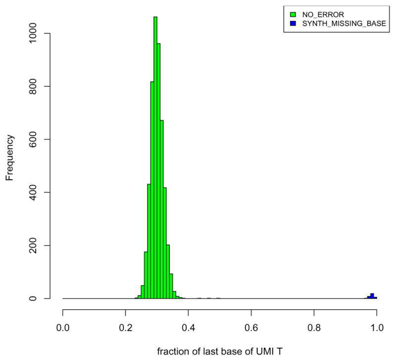
Histogram of the fraction of ‘T’ bases in the last UMI position for each cell barcode. Data from replicate 1 of Batch 1 of Drop-seq was used. For most cell barcodes (green), the fraction of ‘T’ at position 8 of the UMI barcode is drawn from a normal distribution centered around 0.25, consistent with a uniform distribution for all 4 bases. For a small number of the cell barcodes (~5%), a fixation of ‘T’ at the last UMI position is observed (blue).

A command line script to perform this correction has been made publicly available in the Drop-seq website (http://mccarrolllab.com/dropseq/), and its implementation is described in the Drop-seq computational cookbook (http://mccarrolllab.com/wp-content/uploads/2016/03/Drop-seqAlignmentCookbookv1.2Jan2016.pdf)

Digital gene expression

To distinguish cell barcodes that represent genuine transcriptomic libraries arising from cells, rather than from beads never exposed to a cell’s lysate, we ordered the cell barcodes by the total number of transcripts per cell barcode and estimated a “shoulder” in the corresponding plot, as described before (Macosko et al., 2015). All cell barcodes larger than this cutoff were used in downstream analysis, while the remaining cell barcodes were discarded.

We then performed the following steps for every gene within every cell. The UMIs corresponding to all uniquely mapped sense reads (for a given gene) were recorded, and UMIs within an edit distance of 1 (substitutions only) were collapsed, as described in (Macosko et al., 2015). We then counted the number of remaining unique UMIs and this was recorded as the expression count for that particular gene in that particular cell. This resulted in a digital expression matrix (DGE) with genes as rows and cells as columns that served as the starting point for clustering analysis.

Batch correction, PCA analysis, tSNE visualization and clustering

Filtering the expression matrix

The starting pool of 45,000 cells (5,400 cells per replicate in Batch 1 and 11,700 cells per replicate in Batch 2) was first filtered to remove cells where less than 500 genes¹ were detected, and where the proportion of the transcript counts (i.e., UMIs) derived from mitochondrially encoded genes (e.g. Mt-Rnr2, Mt-Co2 etc.) was greater than 10%. We then removed genes that were detected in less than 30 cells, and also those that had fewer than 60 transcripts counts, summed across all the retained cells. These filters resulted in 27,499 cells and 13,166 genes, which were considered for further analysis. From Batch 1, we retained 3,055–3,851 cells from each of the four replicates. From Batch 2, we retained 7,129 cells and 6,383 cells from the two replicates, respectively (Figure S1A, Table S1).

Amongst the retained cells, the median number of genes detected per cell was 810 (IQR 644–1033, Figure S1A, upper panel) and the median number of transcripts counts was 1,192 (IQR 914–1607, Figure S1A, lower panel), and both these numbers were comparable across the different experimental batches and replicates. The median number of transcriptome-mapped reads per cell was 8,200. The median number of reads supporting each detected transcript was 4 (IQR 3–7), but this distribution was very wide (Figure S1B). 95% of non-zero gene-counts in the filtered matrix had a value less than or equal to 3 (75% 1’s, 16% 2’s and 4% 3’s), suggesting that our data (given the shallow sequencing depth) primarily reflected presence/absence of transcripts and did not capture the full dynamic range for most transcripts (Figure S1C).

Transcript counts within each column of the 13,166 genes × 27,499 cell count matrix were normalized to sum to the median number of transcripts per cell (1,192), resulting in normalized counts M_ij for gene i in cell j. For PCA and clustering, we used a log-transformed expression matrix E_ij = ln(M_ij + 1).

QC metrics

A list of quality metrics was obtained for the Drop-seq single cell libraries using Samtools (http://samtools.sourceforge.net/), Picard Tools (http://broadinstitute.github.io/picard/) and in-house scripts. For each single cell library (identified based on its Batch, replicate and a 12bp barcode), we calculated the total number of mapped reads (coding and UTR), the number of genes detected per cell, percentage of the total number of reads assigned to the cell barcode that were from (1) coding regions (2) UTRs (3) intronic regions (4) intergenic regions (5) ribosomal RNA, and (6) mitochondrially derived transcripts. These are summarized in Table S1.

Batch correction

Although the values of E_ij between any two single cells correlated poorly, as expected (Figure S1D), the averaged expression levels of genes and the average counts were highly correlated across the six replicates (Figure S1E–H). However, we noted that the intra-batch correlations were slightly higher than the inter-batch correlations (Figure S1G, H). While no differentially expressed genes were detected between any two replicates from the same batch (e.g., Figure S1E, F), we detected 33 differentially expressed genes at an average expression fold change > 2 between the two batches (FDR < 0.05), most of them expressed at very low levels (see table below). These genes included Xist (the most differentially expressed), Tsix, Hopx and Eif2s3y, all of which are sex-related genes, and Egr1 and Jun, both early response genes to stress and injury. These observations suggest that differences in the proportion of males and females in the two litters, and differences in handling conditions between the two experiments, are therefore likely to contribute to these batch effects in gene expression.

Gene	P-value	log-fold change (Batch 1 vs Batch 2)
Xist	< 1e-6	−3.14
BC033916	< 1e-6	1.87
2810008D09Rik	< 1e-6	1.65
2700089E24Rik	< 1e-6	1.65
Smim10l1	< 1e-6	−1.58
Platr17	< 1e-6	−1.56
A930011O12Rik	< 1e-6	1.52
mt-Rnr2	< 1e-6	−1.37
Mir124a-1hg	< 1e-6	−1.35
Hopx	< 1e-6	1.34
Snhg20	< 1e-6	−1.29
Tsix	< 1e-6	−1.29
Zfp638	< 1e-6	−1.24
Zfml	< 1e-6	1.13
Eif2s3y	< 1e-6	1.09
mt-Rnr1	< 1e-6	−0.99
RP23-102H7.9	< 1e-6	0.87
Rsrp1	< 1e-6	0.86
Eno1	< 1e-6	−0.86
Rpl26	< 1e-6	0.85
2510003E04Rik	< 1e-6	0.85
Egr1	< 1e-6	−0.83
Jun	< 1e-6	−0.82
Kif1bp	< 1e-6	−0.80
Hes1	< 1e-6	−0.78
Gm29609	< 1e-6	0.76
NCBP2-AS2	< 1e-6	−0.74
Gm4792	< 1e-6	0.72
Prss22	< 1e-6	0.70
Sag	< 1e-6	−0.70

We performed batch correction on the expression matrix E_ij using the ComBat method (Johnson et al., 2007) as implemented in the R package sva. ComBat was run using the default parametric adjustment mode, which was able to fit the empirical batch-related variations well according to the author’s recommended prescriptions (the non-parametric mode made slightly better fits, but required more than 4 days running time, compared to less than 10 minutes for the parametric mode on an Intel(R) Xeon(R) CPU, 2.67GHz, 100 GB of memory). The output was a corrected expression matrix $E_{ij}^c$, which was used for PCA and clustering described below after row centering and scaling, resulting in a matrix ${\overline{E}}_{ij}^c$.

Dimensionality reduction using PCA and estimation of significant PCs

The matrix ${\overline{E}}_{ij}^c$ was reduced using principal component analysis (PCA) using the fast.prcomp function in R (package gmodels). PCA computes a low dimensional representation of the high dimensional gene expression data by linearly projecting the expression vectors (columns of ${\overline{E}}_{ij}^c$) along basis vectors that successively maximize the captured variation in the data. The optimal basis vectors are expressed as linear combinations of the row vectors (genes), and are called the “principal directions”. The principal directions can be ordered by their associated eigenvalues, which are proportional to the amount of variance captured. The principal component scores (PCs) of each cell can be obtained by projecting its expression vector along these principal directions. The PC scores of individual cells can be plotted as a scatter graph to visualize cellular heterogeneity in the data along different PCs (representative scatters shown in Figure S1I).

We used a permutation test to identify those PCs that capture statistically significant correlated variation among the genes, which cannot be attributed to random “noise”. Briefly, PCA was performed on 1000 randomized versions of the data, where in each instance, all the rows of the original expression matrix (genes) were randomly and independently permuted. This procedure makes the gene expression values uncorrelated, while maintaining the expression distribution of every gene as in the original dataset. The distribution of eigenvalues of these random matrices agreed very well with the predictions of the Marchenko Pastur (MP) law (Marchenko and Pastur, 1967) which also predicts theoretical upper and lower bounds on the null distribution of eigenvalues (Figure S1J, lower panel). Specifically for a large M × N random matrix (M, N ≫ 0), whose entries are independent, identically-distributed random variables with mean 0 and variance σ², the maximum eigenvalue λ₊ and the minimum eigenvalue λ₋ satisfy the following criteria,

$${\lambda }_{\pm }={\sigma }^2{(1\pm \sqrt{\mu })}^2$$ (1)

Here, $\mu =\frac{M}{N}(\approx 0.486)$ and σ = 1 because of the row scaling operation. The probability density function of eigenvalues PDF(λ) according to the MP law is given by,

$$\mathit{PDF}(\lambda )=\frac{1}{2\pi {\sigma }^2}\frac{\sqrt{({\lambda }_{+}-\lambda )(\lambda -{\lambda }_{-})}}{\lambda \mu }$$ (2)

The values of λ_± and the overall shape of the PDF in our simulated randomized data agreed closely with the predictions of Eq 1 and 2 (Figure S1J, lower panel).

61 eigenvalues in our original dataset had eigenvalues larger than the 2.87, the maximum eigenvalue observed in the randomized data (Figure S1J, upper panel). Since the MP law holds only in the asymptotic limit (M, N → ∞), we only considered the 37 PCs that had eigenvalues larger than 3 (Figure S1J, upper panel, red arrows). The scores of each cell across the top 37 PCs were used for clustering. PCA thus achieves a compression of the expression data from an initial dimensionality of 13,166 (# of genes) to 37 (# of selected PCs).

2-D visualization using tSNE

In order to visualize single cell variation, we generated a two-dimensional non-linear embedding of the cells using t-distributed Stochastic Neighbor Embedding or tSNE (van der Maaten and Hinton, 2008). The scores along the 37 significant PCs estimated above were used as input to the algorithm. tSNE finds two dimensional coordinates for each input data point, such that the pairwise distances between data points in the high dimensional space is conserved in the low-dimensional embedding (Figure S1K). We ran the python implementation of tSNE (https://lvdmaaten.github.io/tsne/) for 2500 steps after disabling the initial PCA step and setting the perplexity parameter to 30. Since tSNE can produce different visualizations in different runs, we ran it once on our full dataset, and used these coordinates only for visualization (i.e., not to identify cell clusters). This step is entirely dispensable if one does not wish to visualize the clusters. We note here that exact tSNE computation has a computational complexity that is O(N²) in the number of input cells, and took ~ 2.5 days to finish on our dataset when run on an Intel(R) Xeon(R) CPU (2.67GHz, 100 GB of memory).

The cells separated into distinct point clouds in tSNE space that were not driven by batch effects (i.e., all point clouds were an admixture of cells from all replicates). However, within some point clouds, there was a visible separation between cells from Batch 1 and Batch 2 (Figure S1K, color scheme same as Figure S1I), suggesting that ComBat did not perfectly correct for batch effects.

Graph clustering and robustness analysis

To identify cell types in the data, we partitioned the cells into transcriptionally similar clusters based on their scores along the thirty-seven significant PCs. We initially used the Louvain community detection method (Blondel et al., 2008), which partitions an input graph to maximize the “graph modularity”, a metric that favors densely interconnected communities and disfavors edges between communities. The Louvain algorithm consists of two steps. In the first step, the method searches for small clusters that maximize the modularity locally. In the second step, it aggregates nodes belonging to the same community, and builds a new graph whose nodes are the aforementioned clusters. The method finds a local minimum of the graph modularity with a computational complexity that scales with the number of cells N as O(N log N). We performed Louvain clustering using the R package igraph.

The input to the algorithm was a k-nearest neighbor (k-NN) graph on the data, where every cell is connected to each of its k nearest neighbors determined based on Euclidean distance in PC-space (using the nn2 function of the RANN package). We weighted each edge in the graph by the Jaccard overlap index of the neighborhood of the corresponding nodes i and j as follows,

$$\mathit{Edge}(i,j)=\frac{\mid {\mathit{Neighbors}}_i\cap {\mathit{Neighbors}}_j\mid }{\mid {\mathit{Neighbors}}_i\cup {\mathit{Neighbors}}_j\mid }$$

Here i and j are nodes, and we refer to this method as “Louvain-Jaccard” in our comparisons below (to distinguish it from the unweighted version, also tested below). While the Jaccard index been used in the past as a similarity measure in graphs, the Louvain-Jaccard strategy has been recently used in studies of social networks (Matutano et al., 2014), and in the Phenograph algorithm, which was developed to analyze mass cyotmetry data from leukemic cells (Levine et al., 2015). We computed the clusters based on a k=30 graph, but extensively evaluated the reproducibility of the output by bootstrapping experiments (below).

The Louvain-Jaccard method identified 30 clusters in our data, which were visualized on the tSNE map by coloring each cell based on its cluster identity (Figure S2A). It’s encouraging to see that the spatial organization of the cells on the tSNE map mirrors the clustering output, given that the tSNE coordinates were not used to influence the clustering.

Reproducibility of clusters

We then used a resampling approach to evaluate the reproducibility of the Louvain-Jaccard clustering. We performed 500 perturbations on the data where in each realization, we,

1. Randomly selected 85% of the cells, and rebuilt the k-NN graph with a randomly chosen k ~ Uniform(15, 100).

2. Removed 5% of the edges, and added 5% spurious edges between randomly chosen cell pairs

3. Added multiplicative noise to each edge by multiplying the edge weight by a random scalar x, where x ~ Uniform(0.6, 1.66).

Clustering using the Louvain-Jaccard method was performed on each of these 500 graphs, and the output cluster labels were recorded. For each Louvain-Jaccard cluster k (=1, 2, …, 30) on the original dataset (i.e. non-perturbed), we calculated two measures of reproducibility – Stability_k and Purity_k (see Appendix 1 for definitions). Stability_k quantifies the extent to which cells from original cluster k are found to cluster together in the randomized trials, and is a value ranging from 0 (randomly distributed) to 1 (found in a single cluster) for each cluster. Low Stability_k values can be indicative of under-clustering. In contrast Purity_k quantifies the extent to which cells from cluster k tend to form an exclusive cluster of their own, ranging from 0 (tend to cluster with other cells) to 1 (tend to cluster largely by themselves). Low Purity_k values are indicative of over-clustering. We desire clusters that have both high values of Stability_k and Purity_k.

All our clusters had high stability values (> 0.92) and most of the major clusters (1–20, ordered by size), containing > 96% of the data, also had high purity values (Figure S2B). Control calculations wherein the initial assignments were randomly permuted (maintaining the cluster sizes) yielded stability and purity values that were, on average, ten-fold lower. Closer examination revealed that some low purity clusters were nearly transcriptionally identical to a closely related high purity cluster (e.g., cluster 18 vs. cluster 1 in Figure S2A) save for 5–10 differentially expressed genes that are likely to reflect technical features (e.g., library size) or sex-related batch effects that were not fully correct by ComBat. For example, clusters 1 and 3 both had a rod bipolar signature (Prkca⁺Car8⁺Scgn⁻Apoe⁻) but were each enriched in cells from Batch 1 and Batch 2 respectively, indicating that batch correction using ComBat was not perfect (Figure S1K). Indeed, the ~10 differentially expressed genes between these two clusters featured Xist, Tsix, BC033916, Ddx3y, Eif2s3y, Fos, Dusp etc. (see table above). Motivated by these observations, we decided to merge clusters that did not show sufficient differential expression.

Merging clusters based on differential expression

We searched for differentially expressed “up” and “down” genes between every pair of clusters using a nonparametric binomial test (see Appendix 2). For each pair of clusters A and B, we evaluated “n”, the number of statistically significant differentially expressed genes (FDR < 0.01), such that there were at least [n/2] genes up-regulated in A and [n/2] down-regulated genes in A, with respect to B. The two-way condition was imposed to avoid subdivision of clusters based on transcriptome quality, although the latter effect was not very prevalent in our dataset. Only genes that satisfied two conditions were considered: (1) Detection in greater than 20% of the cells in at least one of the two clusters (see Note below); and (2) A minimum 2-fold effect size. Here, the effect size was defined as the ratio of the proportion of cells in which the marker was detected between the two clusters (e.g. if gene X is detected in 40% of the cells in cluster A, and 5% of the cells in cluster B, its effect size (A/B) is 8).

The distribution of the number of statistically significant differentially expressed genes “n” between each cluster pair exhibited a “tail” at low values (Figure S2C), likely reflecting effects of library size, strain or biological variation with a type (e.g. cell state). Based on this, we decided to merge every pair of clusters that had fewer than 50 differentially expressed genes each at a minimum effect size of 2 (minimum 25 up and 25 down, FDR < 0.01). We iteratively merged 4 pairs of clusters until all remaining clusters satisfied this criterion, resulting in 26 clusters (Figure S2D). Each pair of the clusters that remained had, on average, 418 differentially expressed genes.

We then tentatively assigned each cluster to a retinal type based on the presence/absence of known markers. We briefly describe the logic behind some of these assignments in Table S2. Clusters 1 and 3–15 were assigned to BC types as they robustly expressed Vsx2 (the marker used for FACS enrichment) and Otx2. Cluster 1 was identified as rod bipolar cells (Prkca+Scgn−) and Clusters 3–15 were identified as cone bipolar cell types (Prkca-Vsx2+), and considered for further validation after assigning each of these clusters to a BC type based on prior knowledge (described in Table S2 in detail). Cluster 2 was identified as Muller Glia (Apoe+Glul+Rlbp1+). Cluster 16 consisted of amacrine cells (Pax6+Tfap2a+). Cluster 17–19, 21 expressed signatures of multiple retinal types (including some of the top genes enriched in clusters 1–15), and considering their low frequency, were annotated as doublets (Table S2). Cluster 20 and 22 consisted of rod photoreceptors (Rho+Pdc+) and cone photoreceptors (Arr3+Opn1sw+). Clusters 23–26, collectively accounting for < 0.5% of the cells, however, expressed non-BC signatures, that we were not able to assign to known types. We did not consider these clusters for validation as based on their frequency such cells would be expected to have extremely wide arbors, and BCs with such morphology have been ruled out by ultrastructural studies till date.

We then compared each of the 26 clusters with the other clusters to identify cluster-specific genes using the binomial test (Appendix 2). Genes detected in a significantly higher proportion of cells in a cluster compared to the remaining clusters (> 2 fold, FDR < 0.01) were ordered by the logarithm of their effect size, and considered for experimental validation (Table S3).

The above test was constructed to find genes that exhibit a binary (ON/OFF) pattern of expression (see Appendix 2, and footnote 3), we used an alternative differential expression test (McDavid et al., 2013) to find ubiquitously detected genes that nonetheless exhibited a quantitative expression difference between clusters (results in a separate worksheet in Table S3). While being less sensitive overall in its ability to identify differential expression amongst lowly detected genes, which dominated our dataset, this test was able to identify cluster-enriched genes that were not nominated by the binomial test (including several genes that were). For example, this test correctly identified Pcp2, Pcp4, Trpm1 and Calm1 as RBC-enriched genes, which were not nominated by the binomial test. These genes were ubiquitously detected in all cells but at much higher levels in the RBCs. For example, Pcp2 was present at 17.3 transcripts per cell on average in RBCs, but at 3.1 transcripts per cell on average in non-RBCs (Table S3). Similarly, this test correctly identified Cabp5 as being enriched in 5A, 5B and 5D but this was missed by the binomial test.

Finslly, we note that thet the threshold of 20%: appears extremely small. We believe this value is justified because the binomial statistics are computed across hundreds to thousands of cells, which can lead to a significant result. The low sequencing depth of our libraries makes dropouts very likely at the individual cell level. However, because of the large number of cells in our data, the PCs capture significant collective correlations, even though individual cells are noisy. The clusters are defined based on these collective signatures, even though an individual gene might be detected in a small fraction of cells within the cluster. Thus we found (and validated) multiple examples of marker genes that detected in only 100 out of 500 cells in a cluster (~20%), but its incidence in the background was less than (0.1%), which is a statistically significant observation.

Selection of candidate RBC genes to test using FISH

For the screen of rod bipolar cell enriched genes, we tested the 10 novel and most enriched genes nominated by the binomial test, and randomly selected 15 genes with robust expression (at least 0.5 average transcripts per cell) among the 100 most enriched genes (Table S3).

Alternative clustering methods and robustness tests

The Louvain-Jaccard method (Blondel et al., 2008; Levine et al., 2015; Matutano et al., 2014) generated reproducible clusters (Figure S2A–D, 1C), many of which were eventually validated as true bipolar types and/or identified as known retinal types (e.g. Müller Glia, rods, cones, amacrines etc). Additionally, we tested alternative approaches to clustering, including recently proposed algorithms for analyzing scRNA-seq data (Grun et al., 2015; Zeisel et al., 2015). We also tested our approach on smaller subsets of our data to explore the impact of sample size on the sensitivity of clustering. We summarize the key results from these explorations here. To facilitate easy comparison across all methods, results are visualized using the tSNE coordinates computed previously (Figure S2E–P). Key differences with regards to the output of the Louvain-Jaccard method (Figure 1C, S2A, D) are noted in each case. The merging step, wherever performed, is explicitly indicated.

• Louvain-Unweighted: (Levine et al., 2015) argued that weighting edges based on the Jaccard similarity metric removes spurious links in the graph and can improve the ability to resolve “natural” clusters in the data. To test this, we repeated the clustering steps using the Louvain algorithm, but using an unweighted 30-NN graph as input (the rest of the steps were identical). This produced 22 clusters, which after the merging step (implemented exactly as described earlier) resulted in 18 clusters (Figure S2E). Encouragingly in this set, the clusters corresponding to the major bipolar types (RBC, BC1A-BC8/9) and Müller glia were conserved. However, many of the clusters with doublet-like signatures could not be resolved (e.g., clusters 17, 19, 21, 23 in Figure S2D) and were merged with another cluster (Figure S2E, red arrows). In addition the rod, cone and rod-doublet clusters were merged into a single cluster (Figure S2E, blue arrows). Thus, in agreement with (Levine et al., 2015), we find that the Jaccard weighting step does remove spurious links especially between transcriptionally proximal clusters relating to cell doublets. Encouragingly in our dataset, none of the true BC clusters that were resolved by the Louvain-Jaccard method were merged together indicating that, transcriptional differences between these clusters are robust and reflected in the structure of the unweighted k-NN graph.

• Infomap: The Infomap algorithm (Rosvall and Bergstrom, 2008) decomposes an input graph into modules by deriving a compressive description of random walks on the graph. The result is a community structure that is represented through a two-level description based on Huffman coding: the first level distinguishes clusters in the network, and the second level distinguishes cells within a cluster. Infomap was implemented in R using code downloaded from http://mapequation.org/.

  The input to the algorithm was an unweighted k-NN graph (k=30). Infomap produced 49 clusters in the initial step (Figure S2F), 19 more than the initial output of Louvain-Jaccard (Figure S2A). A pairwise differential expression test between these clusters exhibited a similar, albeit more accentuated, tail at values < 50 DE genes compared to Figure S2C (not shown). Investigating these clusters revealed that 15 clusters nominated by Infomap were subdivisions of RBC-like cells (cf. Figure S2F), compared to 4 in the case of Louvain-Jaccard (Figure S2A). These clusters shared the RBC-signature (Prkca⁺Sebox⁺Car8⁺Scgn⁻) but differed in the expression of batch driven genes like Xist, Tsix, BC033916, Ddx3y, Eif2s3y, Fos, Dusp etc.. Furthermore, cells within each of these 15 clusters were predominantly derived from one of the two experimental batches (> 80% skew), suggesting that the most likely origin of these extra RBC-like clusters were batch effects, and that Infomap was more sensitive to these signals in the data. It is also notable that, many non-RBC clusters mapped 1:1 between Louvain-Jaccard and Infomap, specifically those retrospectively assigned to BC1A-1B, BC2, BC3A-3B, BC4, BC5A-5D, BC7 and MG (Figure S2A vs Figure S2F).

  Pairwise merging (implemented as before) resulted in 31 clusters (Figure S2G or 1D). Clusters 1–14 were identical between Louvain-Jaccard, Louvain-Unweighted and Infomap (Figure S2D, E, G). A large proportion of small clusters with doublet/contaminant signatures were also reproduced (# 22–31). A key difference was that Infomap split the putative BC8/9 mixed cluster in the Louvain method (Cluster 15 in Figure S2D) into two clusters that we subsequently validated as BC8 and 9, respectively (Clusters 16 and 20, Figure S2G, red arrow).

  The amacrine cell cluster (Cluster 17, Figure S2D) was also split into two clusters corresponding to Glycinergic and GABAergic cells, respectively (Clusters 18 and 21, Figure S2G, blue arrow). Thus, the greater sensitivity of the Infomap method enabled the detection of clusters that were under-represented in the data. Running Infomap using a Jaccard-weighted k-NN graph input resulted in a larger number of initial clusters (65 vs. 50) but post merging the results were identical (not shown). We speculate that Infomap, which is based on random walks on an input graph, is less sensitive to the presence of spurious edges, than the Louvain method, which is based on modularity maximization.

• PCA-2000 + Louvain-Jaccard: Statistically significant PCs, which were used for clustering, were computed based on expression across 13,166 appreciably expressed genes. It is a common approach in scRNAseq studies to pre-select highly variable genes prior to PCA/clustering (e.g. (Macosko et al., 2015; Zeisel et al., 2015)). We used Ziesel et al.’s approach to select 2,000 highly variable genes in the data (based on fitting a relationship between mean vs. coefficient of variation of all genes), and repeated the PCA using only the expression of these genes. This was followed by Louvain-Jaccard clustering using significant PCs, estimated using a permutation step. The results after the merging-step (Figure S2H) agree closely with the original results (Figure S2D), with the exception that 3 doublet clusters (blue arrows in Figure S2H) were merged with larger clusters. Overall, this suggested that a smaller, highly variable subset of the genes was sufficient for resolving the most important clusters, but with a decreased sensitivity towards identifying cell doublets.

• k-means clustering in PCA-space: To evaluate whether a simpler, faster method could resolve the clusters when the number of clusters was specified, we performed k-means clustering using the 37 significant PC scores as input (with k chosen to be 30 based on the Louvain-Jaccard output). The raw output of k-means clustering (Figure S2I) was significantly different from that of Louvain-Jaccard, pre-merging (Figure S2A). Specifically, we found that 9/30 of the clusters were subsets of the RBC cloud (2, 4, 6, 9, 11, 13, 14, 15, 25), while 4 clusters comprised Müller glia (#12, 16, 17, 22). Additionally, we found a few clusters that were an admixture of validated types. BC types 1B and 2 were merged into a single cluster (Figure S2I, blue arrow) as were BC types 3B and 4 (Figure S2I, red arrow) (cf. Figure 1C–1D). Furthermore, most of the cell doublet clusters and contaminant clusters were not resolved. We speculate that the non-uniform/non-Gaussian distribution of the cells in expression space underlies the inferior performance of parametric methods like k-means over graph clustering methods. We also emphasize here that the apparent computational efficiency of k-means clustering presumes that an appropriate value of k is known. If not, an additional layer of computation is necessary to select an optimal value of k, the number of clusters (e.g., using methods like the gap statistic), which can substantially increase computational time.

• tSNE+DBSCAN: Similar to (Macosko et al., 2015) we performed density clustering using DBSCAN on the tSNE coordinates as input (eps=1.8, minPts). As before, parameters were tuned so that the main point clouds on the tSNE map were assigned to distinct clusters. At these, values, many small clusters of < 6 cells were detected, resulting in 72 clusters (Figure S2J).

  Conceptually, this approach assumes that the output of tSNE, a visualization technique, faithfully represents the cluster structure of the data. While we have found empirically in the current and past work that distinct cell types in the retina project onto well-separated point clouds in tSNE, this need not be generally true when cell types/states occupy a more continuous spectrum (e.g., in hematopoiesis). On the practical side, the tSNE embedding can change based on stochastic initialization, which makes it hard to compare the output on bootstrapped versions of the data, especially if the choice of density clustering parameters is tuned to the visualization. Lastly, exact tSNE computation time and memory requirements scale with the number of points N as O(N²) which can become prohibitively long for even 50,000 data points. An approximate tSNE algorithm is available, but in practice, produces less well-separated point clouds in practice compared to the exact method. In contrast, the visualization-independent graph clustering methods have a computational and memory footprint that is between O(N) and O(N log N), making it highly scalable for larger datasets (Fortunato, 2010).

• Clustering on Batch 1 cells: We explored the ability to detect major bipolar clusters on smaller subsets of the data. We ran our clustering pipeline on 13,938 cells from the first biological batch (49% of our data). As in the case of the full dataset, we first ran PCA on the median-normalized and log-transformed expression matrix of these cells (skipping batch correction). The resulting significant PCs were used to find clusters using both the Louvain-Jaccard and Infomap algorithms (using a 30-NN graph). The results following the cluster-merging step, which was implemented using the same parameters, are show in Figure S2K (Louvain-Jaccard) and Figure S2L (Infomap, also see Figure 1E). Only cells that were included in the analysis are shown in the tSNE plots.

  In this setting, both methods suffered only slight loss of sensitivity and were able to resolve most of the BC clusters as in the full dataset. Louvain-Jaccard was unable to resolve the BC5B and BC5C clusters (Figure S2K, blue arrow). Infomap fared relatively better, and was able to resolve these clusters (Figure S2L, blue arrow). However, when compared to its output on the full dataset, it was unable to resolve BC8 vs. BC9 (Figure S2L, red arrow).

• BackSPIN: Originally proposed by (Zeisel et al., 2015), BackSPIN is a biclustering method that based on the SPIN algorithm to sort rows and columns of a correlation/distance matrix. BackSPIN begins by sorting the cell-cell correlation matrix evaluated based on a subset of highly variable genes, and then splits the matrix into two groups of cells if a splitting parameter exceeds a user-defined value (Default value 1.15). Genes are partitioned into the two splits based on their average expression. The procedure is then successively repeated on each of the partitions until the number of splitting cycles exceeds a user defined threshold m. m split cycles results in a maximum of 2^m clusters.

  We implemented BackSPIN using publicly available code (https://github.com/linnarsson-lab/BackSPIN) using the default parameters. We used the function feature_selection to select 2,000 highly variable genes (same set used in 3. above), and used the median-normalized, batch corrected and log-transformed expression matrix $E_{ij}^c$ as input to the function backSPIN. The algorithm took longer than 7 days to run on the full dataset (27,499 cells), so we elected to run it on the 13,938 cells from Batch 1, up to six cycles (runs were performed on an Intel(R) Xeon(R) CPU, 2.67GHz, 100 GB of memory).

  The clustering output of the BackSPIN algorithim, consisting of 10 clusters, is visualized in Figure S2M. BackSPIN successfully separated RBC, Müller glia and large cone bipolar clusters corresponding to BC5A, BC6 and BC7. However, it reported the following cases as single clusters (1) BC1A, BC1B, BC2, BC8/9 (Figure S2M, red arrows); (2) BC3B, BC4, BC3A (Figure S2M, blue arrows); (3) BC5B, BC5C and BC5D (Figure S2M, green arrows); and (4) Rods/Cones and Amacrine cells (not indicated).

  We speculate that the inability of BackSPIN to resolve these clusters relates to the default value of its minimum splitting score (parameter k in the function backSPIN, defaults to 1.15). Preliminary tests indicated that lowering the value of this parameter could potentially resolve more clusters, but exploring a rigorous, data-driven way to choose the optimal value of this parameter for our dataset was not obvious, and also beyond the scope of this work.

  Clustering on 5,000 cells from the first batch: To further explore the effect of sample size on the sensitivity of clustering, we tested our methods on 5,000 randomly sampled cells from the first batch (18% of our data) after normalization and PCA. The clustering output of Infomap is shown in Figure S2N (as in 6. Louvain-Jaccard exhibited lower sensitivity and is not shown). Compared to its performance on 13,938 cells, Infomap reported BC5B/BC5C, BC3B/BC4 and rods/cones respectively as single clusters (Figure S2M, blue, red, and green arrows respectively), and additionally was unable to detect the amacrine cluster (black arrow). It also failed to resolve members of the “doublet clusters” and merged them into larger clusters because they were poorly represented in this dataset. Interestingly, Infomap was still able to resolve the BC8/9 (Figure S2N, cluster 15), although only 56 cells of this cluster were present in the data.

  BackSPIN’s performance on this dataset (Figure S2O) was slightly worse on this dataset compared to its performance on the 13,938 cells (Figure S2L, arrows). In addition to the shortcomings listed in 7., it was unable to fully resolve the BC6 cluster (Figure S2L, black arrow).

  RaceID: RaceID (Grun et al., 2015) was developed to enable the identification of rare and abundant cell types from single cell RNA-seq data. Here, we disabled the rare cell type identification step, and only ran the first step of RaceID. To identify abundant cell types, the algorithm uses the k-means method to find clusters on expression data. The optimal number of clusters is calculated using the gap statistic method.

  We ran the publicly available implementation of RaceID (https://github.com/dgrun/RaceID) with mintotal = 600, minexpr=5, minnumber =1, maxexpr=500 (all other parameters were set to their default values). Because of its long running time (due to the gap statistic calculations), RaceID could only be run on the 5,000-cell dataset (2123 genes selected), and took 4 days to complete on an Intel(R) Xeon(R) CPU, 2.67GHz, 100 GB of memory. The clustering output of RaceID is shown in Figure S2P, and consisted of 4 clusters (chosen by the gap-statistic method), two of which were divisions with the RBC cluster. The remaining two clusters were an admixture of BCs and Müller glia (Figure S2P). We speculate that RaceID fails to identify meaningful clusters because of the poor performance of k-means clustering on the raw, high dimensional data. Indeed, we also observed that the performance of graph clustering algorithms deteriorated when applied directly to the raw data, likely because of the noise in nearest neighbor estimation in high dimensional spaces. Thus PCA, in addition to reducing the dimensionality of the data to a meaningful representation, also serves as a “de-noising” step.

Comparison with full retina Drop-seq (Macosko et al., 2015)

To assess the reproducibility of Drop-seq and the performance of our computational pipeline, we reanalyzed cells from the eight bipolar cell clusters identified in the full retina Drop-seq study (Macosko et al., 2015). We asked whether the difference in the number of clusters reflects lack of reproducibility, larger cell number in the current dataset, and/or improved clustering methods.

Macosko et al. identified 39 clusters from 44,808 retinal cells using the tSNE + DBSCAN approach. These included 8 Vsx2⁺Otx2⁺ bipolar clusters (26–33) that comprised 6,285/44,808 cells. Of these, clusters 27–33 had a cone-bipolar signature (Scgn⁺Prkca⁻) and cluster 26 comprised rod bipolar cells (Scgn⁻Prkca⁺). We removed cells that contained fewer than 500 detected genes (n=810) or greater than 10% mitochondrially-derived transcripts (n=8). The remaining 5,466 cells had a median 1,035 detected genes. We considered 12,318 genes detected in greater than 20 cells, and clustered the original expression matrix based on the following procedure,

(1) Correct for batch effects using ComBat (7 batches); (2) z-score (standardize) gene values and find significant PCs using a permutation test (20 found); (3) Build a 30-NN graph and cluster using Infomap; (4) Iteratively merge clusters pairwise based on differential expression. (We elected to use Infomap rather than the Louvain-Jaccard method as it demonstrated greater sensitivity on smaller datasets in our downsampling experiments).

Infomap detected 16 clusters, which were visualized on a tSNE map computed from the PC scores (Figure S3A) (Note. These were recomputed and are not the coordinates published in (Macosko et al., 2015)). Types were assigned to these clusters based on top differentially expressed markers (binomial test) following the heuristics detailed in Table S2. Coloring the tSNE map with the original cluster identities (Figure S3B) from Macosko et al. showed that closely related bipolar types had been lumped by the original analysis (e.g., BC1A-1B, 2-3A etc.), but were resolved when analyzed in isolation using our present computational approach. 12/16 clusters were comprised of BCs, and the remaining four included non-bipolar cells, cell doublets, or dying cells that were likely misclassified in the original dataset. We also noticed some variation within clusters – for example, some RBCs expressed higher levels of rod genes (e.g. Prkca, Sag) and mitochondrially encoded genes (e.g. mt-Co2, mt-Rnr2) suggesting these could be a combination of doublets and apoptotic cells (Figure S3A, dashed ellipsoid). Lastly, we note that despite analyzing BCs in isolation, the different types do not perfectly segregate on the tSNE map, reflecting the limitations of the tSNE + DBSCAN approach.

To understand how closely the assigned types in the full retina data matched the corresponding types identified in the bipolar data presented in the present work, we computed the Pearson correlation coefficient between the average expression values of the major Louvain-Jaccard clusters identified in the Vsx2-GFP Drop-seq dataset (Figure 1C) against the clusters identified in the full retina Drop-seq dataset by Infomap (Figure S3A). Figure S3C shows that the expression vectors of corresponding types are highly correlated (r > 0.88), reflecting the robustness of gene signatures among similar cell types between the two datasets. Also, clusters that are a mixture of closely related types in the full retina data, show a similar high correlation with the corresponding clusters in the bipolar data (e.g. the BC5B+5C cluster in the full retina data shows high correlation with both the BC5B and 5C clusters in the Vsx2-GFP data; and similarly the BC3B+4 cluster shows high correlation with both the BC3B and 4 clusters in the Vsx2-GFP data).

Two reasons could underlie the imperfect classification in the full retina Drop-seq data compared to the bipolar data: (1) The smaller number of cells; and (2) the quality of the transcriptome data. Here, we found that almost all of the cells had abundant levels of rhodopsin expression, likely due to cross-contamination (rods constituted > 65% of cells in the dataset and are often damaged during tissue dissociation, with the result that rod transcripts are abundant in ambient, cell-free RNA) (Figure S3F). In contrast, the levels of rhodopsin were low in most clusters except those classified as rods in the bipolar data.

Using Drop-seq clusters to train a Random Forest classifier

Analysis of smaller subsets of our Drop-seq dataset (Figure S2K,L,N) and the full retina dataset (Figure S3A) suggested that as sample size decreases, it becomes challenging to resolve distinct cell types. While cell types like RBCs or Müller Glia are easily classifiable because of their distinct transcriptional signatures, our experiments above foreshadowed the possibility that in smaller datasets closely related types like BC3B/4 or BC5B/5C are likely to be lumped into single clusters. We reasoned that a supervised classifier trained on the cluster signatures from the Vsx2-GFP Drop-seq dataset could be useful to further resolve independent datasets where unbiased clustering is likely to be insufficient.

We used our Louvain-Jaccard cluster labels to train a random forest classifier on our Vsx2-GFP Drop-seq dataset. A random forest (Breiman, 2001) is an ensemble learning method that consists of a multitude of decision trees, each trained on a random “bag” of features (here, genes). We composed a “training set”, sampling cells from 18 major clusters in the primary Drop-seq data: Clusters 1–16, 20, 22 (Figure 1C), which represented all 13 BC types (BC8/9 was treated as a single cluster), RBCs, Müller Glia, amacrine cells, rod and cone photoreceptors. The number of cells from each cluster k that was included in the training set N_k was chosen such that N_k = min(300, 0.4* |cells_k|), and thus at most 40% of each cluster was used for training. The training set was comprised of 3,990 cells (14.2% of our dataset) and we used the z-scored expression vectors of these cells’ columns of Ē_ij. The remaining 24,004 cells were used to test the performance of the trained classifier.

We trained a random forest using 1,000 trees on the training set using the R package randomForest. Stratified sampling was used to ensure that all classes were equally represented in training each of the composite trees. The median “out-of-bag” error rate of the final classifier, which quantifies the quality of the model, was less than 2% for all the 18 classes (median value 0.8%). Finally, we tested the trained model on the 24,004 cells (test set) that were kept aside, whose labels were independently known from the original clustering, but not used to build the classifier. We used the model to assign a class label (one of 18 possible labels) to each cell, but considered this a valid assignment only if the majority vote was composed of a minimum of 15% of the trees in the forest (with 18 class labels, even a ~5.5% vote could constitute a majority). Based on this criterion, 214 cells in the test set could not be classified into a definitive class (0.9%). The classification error rate for the remaining cells was strikingly low with a median per-class-misclassification rate of 1%. Figure S3D shows a “confusion matrix” for this classification, whose diagonal structure reflects the robustness of the classifier.

Lastly, we used this model to classify each cell in the full retina dataset. As before, we assigned each cell to the class with the majority vote, only this comprised > 15% of the trees. Our results (Figure S3E) show that in nearly all the full retina clusters, a majority of the cells could be classified to the type that was consistent with their labeling based on top differentially expressed markers (Figure S3G). Clusters combining cells from two types (BC3B/4, BC5B/5C) were decomposed into these types by the classifier. Only two clusters contained a majority of cells (>80%) that could not be classified: these clusters had a high expression of photoreceptor genes (Figure S3F). Taken together, these results show that type-specific gene expression signatures were faithfully and robustly reflected in the expression levels of individual cells from the putative corresponding type, rather than just cluster averages or over-fitting within a dataset (Figure S3C).

Dendrogram

Average expression vectors were calculated for all the 15 bipolar clusters. For each cluster, we averaged the normalized gene counts M_ij across all the cells, and then log-transformed this value after the addition of 1. We then removed all genes whose average expression values were lower than 0.1 across all clusters, and/or that did not show sufficient variability in these values (CV < 0.1). This resulted in 3,839 genes. Slight variations in these parameters did not affect qualitative results. The average expression vectors including these genes were hierarchically clustered using the R package pvclust (Euclidean distance, average linkage), which provides bootstrap confidence estimates on every dendrogram node, as an empirical p-value over 10,000 trials (Figure 1G, 6B). Euclidean/Correlation based distance and Average/Complete linkage yielded consistent dendrograms.

GO-PCA

Significantly enriched Gene Ontology (GO) terms with the top principal components in the Drop-seq data were computed using GO-PCA, an unsupervised method to mine key signatures in gene expression data (https://github.com/flo-compbio/gopca) (Wagner, 2015). We considered only the 14 Louvain-Jaccard clusters of BCs, and the three clusters corresponding to rods, cones and Müller glia in this analysis (Figure 1C).

We used our cluster labels to generate multiple cell-averaged gene signatures for each of the 17 clusters, as a means to suppress sampling noise in measurements of individual cells. Briefly, we sampled N instances of m randomly chosen cells from each cluster, and in each case instance averaged the expression vectors of the m chosen cells. For c clusters, this yields N*c expression vectors each of which is an m-cell averaged gene signature. We chose N=200, and m=20 for the BC and Müller glia clusters, and m=5 for the rod and cone clusters, as the latter were smaller in size. The resulting 13,166 genes x 3400 input matrix was used as input to GO-PCA, which was run with the default parameter values (see https://gopca.readthedocs.org/en/latest/running.html#running-go-pca-go-pca-py). GO-PCA was performed twice, once on only the BC meta-clusters (Figure 6C, Table S5), and a second time by including the photoreceptor and Müller glia meta-clusters (Figure S7A).

COMPUTATIONAL METHODS SMART-SEQ2 DATA

Vsx2-GFP Smart-seq2 data analysis steps

288 single-cell libraries and 4 bulk libraries were sequenced. Expression levels of gene loci were quantified using RNA-seq by Expectation Maximization (RSEM) (Li and Dewey, 2011). Raw reads were mapped to a mouse transcriptome index (mm10 Ensembl build) using Bowtie 2 (Langmead and Salzberg, 2012), as required by RSEM in its default mode. On average, 93% of the reads mapped to the genome in every sample (range 91.8–94.6%), and 63% of the reads mapped to the transcriptome (range 53.5–71.8%). RSEM yielded an expression matrix (genes x samples) of inferred gene counts, which was converted to TPM (transcripts per million) values and then log-transformed after the addition of 1 to avoid zeros.

We considered 229 single cell libraries that satisfied the following QC criteria: > 500K genome mapped reads, genome mapping rate > 50%, transcriptome mapping rate > 25%, % intergenic reads < 20%, read duplication rate < 10%, > 2,000 genes detected (including only genes that are detected in at least 5 cells), rRNA rate < 10%. The final expression matrix consisted of 14,191 genes and 229 cells. These cells altogether accounted for 183 million mapped reads, which was roughly 80% of the amount of mapped reads in the Drop-seq cells.

As in the case of the Drop-seq dataset, we used PCA to reduce the dimensionality of our expression matrix after standardizing each row. 10 significant PCs were identified by a permutation test, and these PCs were used to cluster the cells based on the Infomap method (k=15) and also to independently embed these cells on a tSNE map (Figure 7E). (The Louvain-Jaccard method yielded similar results). We then used the random forest classifier trained and validated on the Drop-seq dataset to classify each individual cell based on its scaled expression vector. The class assignment was completely agnostic to the output of the clustering or its location on the tSNE map. A cell was assigned to a class (out of 17 possible classes) based on majority vote, only if it constituted > 15% of the trees in the random forest. 2/229 cells failed to be classified. The remaining 227 cells were classified into nearly all of the expected types in the Vsx2 transgenic line in expected proportions featuring RBCs (n=99), MG (n=22), BC1A (n=14), BC1B (n=4), BC2 (n=3), BC3B (n=8), BC4 (n=9), BC5A (n=24), BC5B (n=2), BC5C (n=11), BC6 (n=16), BC7 (n=8), BC8/9 (n=5), amacrine cells (n=1), rod photoreceptors (n=1). Notably, none of the cells were classified as BC3A or BC5D.

Encouragingly, all the moderately sized clusters (n > 10) by the PCA+Louvain-Jaccard method either consisted of a single RF type (Figure 7E, e.g., RBC, BC5A, MG) or, more often, of two closely-related types (e.g., BC3B-BC4 or BC1A-BC1B). This enabled us to use the Drop-seq signatures to deeply resolve the Smart-seq2 data, which were not fully possible using unbiased approaches. Using the RF class assignments, we then searched for differentially expressed genes for each of the BC types that had at least five cells and MG using a likelihood ratio test (McDavid et al., 2013). Briefly, cells in each cluster were compared against the remaining cells and significantly upregulated genes at an average expression fold change of at least 2 were recorded (FDR < 0.01). The top differentially expressed genes in all clusters were identical to those nominated by Drop-seq.

Taken together, these results underscore the reproducibility of our classification across multiple datasets. When the quality of the unbiased classification is compared to the classification on the 13,000 and 5,000 cell Drop-seq data, these results also suggest that when the goal is to classify a heterogeneous tissue into cell types, it is far more beneficial to sequence a much large number of cells at a shallow depth than to distribute those reads across a few cells.

Kcng4-cre;stop-YFP Smart-seq2 data analysis steps

Raw reads from the 384 single-cell RNA-seq libraries were mapped and quantified as described in the previous section. 309 single cell libraries that satisfied the following QC criteria were considered for further analysis: > 500K genome mapped reads, genome mapping rate > 50%, transcriptome mapping rate > 30%, % intergenic reads < 20%, read duplication rate < 10%, > 2,000 genes detected (including only genes that are detected in at least 5 cells), rRNA rate < 10%. The RSEM expression matrix (log(TPM+1) units) consisted of 14,191 genes and 309 cells, sequenced to a typical depth of 1.07 million transcriptome-mapped reads. On average 75% of the reads mapped to the genome in every sample, while 47% of the reads mapped to the transcriptome and 6,388 genes were detected per cell.

We performed PCA+Infomap clustering followed by merging (yielding 4 major clusters) and visualization on tSNE as described in the previous section. Random forest classification was performed on each cell using its expression vector, but with the following key difference in normalization. Gene expression values (log(TPM+1) units) were not standardized using the mean (μ) and standard deviation (σ) within the Kcng4-YFP dataset. Instead, for every gene we computed μ and σ using the 229 cells Vsx2-GFP Smart-seq2 dataset, and used these quantities to standardize (subtract μ and divide by σ) the corresponding gene expression values in the Kcng4-YFP+ cells. Since the random forest classifier was trained on standardized Vsx2-GFP cell signatures of Drop-seq, we reasoned that Smart-seq2 measurements from the same biological source would serve as the most appropriate background model for feature normalization prior to classification.

The normalized expression vector of each cell was used to query the random forest model for one of 18 possible class labels. As in the previous section, a cell was assigned to a class only if its majority vote comprised > 15% of the trees in the random forest. Here we found that a majority of cells within one of the four large clusters (n=82) failed to be classified unequivocally (Figure 7G). Examination of their gene signatures showed that these cells coexpressed Type 5 (Cabp5, Grm6, Kcng4) and rod photoreceptor markers (Rho, Pdc, Gnat1), suggesting that these could be cell doublets. Majority of cells in each of the three remaining clusters classified into a single class; these comprised BC5A (n=110), BC5D (n=60) and BC7 (n=43), consistent with our type assignments of these clusters based on the differentially expressed genes (Sox6 and BC046251 in BC5A, Lrrtm1 and Kirrel3 in BC5D, Igfn1 and Kcnab1 in BC7) (Figure 7H,I).

Assessment of cluster stability and purity

The “cluster stability index” defined as,

$${\mathit{Stability}}_k=1-\left(\frac{1}{500}\right)\sum _{i=1}^{500}\frac{H_i^k}{H_i^{\mathit{Tot}}}$$

where $H_i^{\mathit{Tot}}$ is the overall Shannon diversity index (entropy) of the cluster distribution of cells in realization $i{\left\{p_j\right\}}_{j=1}^{N^i}$ and N_i is the number of clusters found in realization i by Louvain-Jaccard, before merging. Then,

$$H_i^{\mathit{Tot}}=-{\sum }_{j=1}^{N^i}{p}_j\text{log}(p_j)$$

$H_i^k$ is the Shannon diversity of the cluster distribution of only the cells belonging to cluster k in realization $i{\left\{f_j^k\right\}}_{j=1}^{N^i}$.

$$H_i^k=-{\sum }_{j=1}^{N^i}{f}_j^{k}log(f_j^k)$$

As the formula suggests a cluster is “stable” if $H_i^k$ is much less than the background entropy $H_i^{\mathit{Tot}}$.

The “cluster purity index” is defined as,

$${\mathit{Purity}}_k=\left(\frac{1}{500}\right)\sum _{i=1}^{500}\frac{\mid {\mathit{cells}}_k\subset {\mathit{cells}}_{\mathit{clust}(i,k)}\mid }{\mid {\mathit{cells}}_{\mathit{clust}(i,k)}\mid }$$

where, clust(i,k) denotes the cluster in realization i that contains the maximum proportion of cells from the original cluster k. cells_k denotes the cells that comprise cluster k.

As an illustration, consider two situations: (1) Cells from cluster k are found to form three clusters each consisting of only cluster k cells; and (2) Cells from cluster k are found to all be assigned to a large cluster that contains cells from additional clusters. The former situation would lead to low Stability_k but high Purity_k, while the latter situation would lead to high Stability_k but low Purity_k.

We emphasize that the quantities Stability_k and Purity_k attempt to provide a quantitative answer to the following question: Does a clustering method provide consistent answers when only a fraction of the cells are used for clustering, and/or when the underlying input graph is noisy? In other words, they merely evaluate the reproducibility of a particular method’s output (e.g., Louvain-Jaccard) to perturbations in the input dataset. High values of these metrics are necessary but not sufficient conditions for the output of a clustering algorithm to be valid. Indeed, it is possible that two clustering methods produce different solutions, each of which is both “stable” and “pure”. Which of these answers is correct, if at all, can only be resolved with further validation and testing that is independent of the principal dataset itself. Nevertheless, the convergence of multiple different methods to a similar solution could be construed as an encouraging sign (as was the case of the Louvain-Jaccard and Infomap algorithms tested on bipolar cell data).

Binomial test for differential expression

Consider the case wherein we wish to ascertain if a gene g is expressed more frequently in subpopulation A (N cells) compared to a second subpopulation B (M cells). Suppose gene g is present in N_g/N in subpopulation A and in M_g/M cells in supopulation B (>= 1 transcript/cells). To test whether gene g is a marker for subpopulation A with B as reference, we compute the following p-value,

$$p_g=\sum _{k=N_g}^N\left(\begin{array}{c}N\\ k\end{array}\right){\gamma }^k{(1-\gamma )}^{N-k}$$

Here, γ = M_g/M is the detection frequency in subpopulation B. A low p-value indicates that g is present in A cells with a much higher frequency than can be explained by its frequency in subpopulation B. To avoid spurious significance calls where M_g=0 but N_g is small (e.g., 1 or 2), we added a pseudocount of 1 whenever M_g = 0. This filters out genes that are extremely lowly expressed in both populations. In comparing two populations, we only considered genes that satisfied a minimum effect size defined as e = (N_g/N)/(M_g/M) ≥ 2. We computed the nominal p_g for all valid genes and converted these to FDR values. A gene was considered statistically significant if it satisfied FDR < 0.01.

A similar test can be performed to find genes that are enriched in B compared to A. To find marker genes for subpopulation A against all the other cell types in the data, we pooled the cells from all the subpopulations except A, and regarded this pool as subpopulation B.

Note: This test is only suitable for finding genes that exhibit a binary (ON/OFF) pattern of expression. Specifically, it is incapable of nominating genes that are expressed in both cell types but at different quantitative levels. Moreover, the test, in its current formulation, does not differentiate between different quantitative levels of transcript expression (e.g., two cells that express two and five transcripts of a gene are regarded as equivalent). This makes the test conservative, and particularly suited to datasets consisting of a large number of cells, where in each case only a small portion of the transcriptome is captured. For example, in the current dataset, a gene, when expressed in a cell, was usually present 90% of the time at a transcript count ≤ 3. Each reported transcript had on average 4 supporting reads (IQR 3–7), making these counts highly reliable.

Lastly, we note that test can be easily generalized to multinomial versions that account for expression levels.

QUANTIFICATION AND STATISTICAL ANALYSIS

For the Drop-seq experiments, cells were collected from five and four Vsx2-GFP mice during first and the second batch, respectively. In both batches, single cell suspensions from dissected retinas were pooled and sorted for GFP+ cells. For the Vsx2-GFP Smart-seq2 experiments, left and right retinas from one Vsx2-GFP mouse and the left retina from another mouse were dissected, suspended and separately processed using FACS to prepare three 96-well plates of single cells. Bulk populations of ~10,000 cells were also sorted from each retina. For the Kcng4-cre;stop-YFP Smart-seq2 experiments, four retinas from two animals were dissected, suspended and separately sorted into four 96-well plates of single cells. For the Tg(Htr3a-EGFP)#aShkp) bulk RNA-seq experiments four retinas from two animals were used for each of the two replicates.

For experiments involving FISH or immunohistochemistry, retinas were from two or more animals for each experiment. Sections were obtained from the vicinity of the optic nerve, Approximately 80 retinas were used for histological analysis.

Statistical methodologies and software used for performing various types analysis in this work are cited where appropriate in the Methods text. Most of the analysis was performing in R, but python was used for certain tasks (e.g. running the tSNE algorithm and the BackSPIN algorithm. Expression patterns of genes across cell clusters are shown in dotplots (e.g. Figure 1F), which simultaneously depict the fraction of cells in a cluster (row) that express a particular marker (column) based on the size of the dot, and the average number of transcripts in the expressing cells based on the color scale, as indicated in the legends. In the dendrograms, asterisks denote statistical significance as assessed by empirical p-values calculated using bootstrap (*, p < 0.1; **, p < 0.01; ***, p < 0.001; ****, p < 0.0001).

Differential expression of genes across clusters in the Drop-seq data was evaluated using the binomial test (see above). Differential expression of genes in the Smart-seq2 dataset was evaluated using the method described in as used in our previous work (McDavid et al., 2013). The binomial test could not be used here because of the nature of the data (full transcript length, and non-UMI). We employed multiple hypothesis correction wherever significance was evaluated across multiple statistical tests, using an FDR threshold of 0.01.

DATA AND SOFTWARE AVAILABILITY

Data Resources

Raw and processed data files for Drop-seq and Smart-seq2 experiments are available under the GEO accession number GSE81905.

R Markdown code for reproducing clustering analysis

As an accompaniment to this paper, we provide an R markdown file that describes step-by-step instructions starting with loading and preprocessing the Drop-seq digital expression matrix, PCA, clustering based on Louvain-Jaccard and Infomap, and data visualization. The digital expression matrix and functions necessary to run these commands are also provided as an R data file and an R script respectively and can be accessed at https://github.com/broadinstitute/BipolarCell2016.

Supplementary Material

1. Figure S1. Library complexity metrics, correlation between replicates, PCA and tSNE, related to Figure 1.

(A) Violin plots of genes/cell (upper) and transcripts/cell (lower) across the six experimental replicates. Only 27,994 cells filtered based on QC criteria are included (individual points). (B) Histogram of the ratio of the number of observed reads and the number of observed UMIs for the nonzero entries of the digital expression matrix (DGE). Dashed read line shows the median value. Both axes are represented in logarithmic units. (C) Histogram of the values of non-zero transcript counts observed in the DGE. y-axis is represented in logarithmic units. (D) Scatter plot of gene expression values before batch correction (E_ij units) between two cells randomly chosen from Batch 1 replicate 1. Each dot corresponds to a gene, and many genes have similar values because of the digital nature of the data. (E) Scatter plot of average gene expression values (across cells) between replicate 1 and replicate 4 of Batch 1 (F) Same as E. for replicate 1 and replicate 2 of Batch 2. (G) Same as E. for Batch 1, replicate 1 and Bach 2, replicate 1. Representative genes that are differentially expressed are indicated (full list in Table S2). (H) Sample-sample correlation (Pearson) of cell-average gene expression values (E_ij, upper triangular), and of non-normalized cell-average transcript counts (lower triangular), before batch correction. For panels (E–H), average expression values for every gene within a sample were computed by first averaging the normalized transcript counts M_ij across all the cells, adding 1 and then taking the logarithm. Only 13,166 significantly expressed genes were considered. (I) Scatter plots of PCA-scores for PC1–PC2, PC3–PC4 and PC9–PC10. Each dot corresponds to a single cell, and is colored based on its sample of origin (legend) (J) PCA - eigenvalue spectrum computed using the real expression matrix (upper) and randomized (n=500) expression matrices (lower). The theoretical spectrum based on the Marchenko-Pastur (MP) law is shown in red in the lower panel. The empirically observed (rand) and the predicted (MP) maximum and minimum eigenvalues λ₊ and λ₋ for the randomized data are indicated (see Equations (1) and (2) in Supplementary Experimental Procedures). Eigenvalues that are larger than the empirical-bound are indicated with red arrows (upper) (K) 2D visualization of single cell variation using t-distributed stochastic neighbor embedding (tSNE), computed based on cell scores along 37 significant PCs. Single cells are colored based on their sample of origin and the scheme is the same as in panel I.

10. Table S1.

Quality metrics of Drop-seq single cell libraries used for clustering analysis, related to Figure 1

11. Table S2.

Summary of previously known markers for bipolar cell types (with references) and description of assignment of computationally identified clusters to specific types, related to Figure 1

12. Table S3.

List of differentially expressed genes in each of the 26 Louvain-Jaccard clusters, relative to the rest of the cells in the Drop-seq dataset partitioned by large and small effect sizes, related to Figure 2

13. Table S4.

Sequences of primers used in PCR to generate template for in vitro transcription of antisense riboprobes, related to Figure 2

2. Figure S2, Bootstrap analysis of Louvain-Jaccard clusters, and comparison of six clustering methods, related to Figure 1.

(A) Clustering output of Louvain-Jaccard, prior to merging proximal clusters (B) Stability_k and Purity_k scores for Louvain-Jaccard clusters in A. (C) Histogram of the number of differentially expressed genes (based on a binomial test described in Supplementary Experimental Procedures, FDR < 0.01) found in all pairwise comparisons of clusters in panel A (N= 2915 comparisons). In each pairwise comparison, only genes detected in at least 20% of cells in at least one of the two clusters, and exhibiting an effect size > 2 were considered. The median number of differentially expressed genes (DE) in a pairwise comparison was 418 (red dashed line). Inset shows that a small number of clusters have fewer than 50 DE genes. (D) Louvain-Jaccard clusters, after iteratively merging clusters with fewer than 50 DE genes (henceforth referred to as the “post-merge”), identical to Figure 1C. (E) Louvain clusters based on an unweighted k-NN graph, post-merge. (F) Clustering output of Infomap, without merging. (G) Infomap clusters, post-merge, same as Figure 1D. (H) Post-merge Louvain-Jaccard clusters, based on significant PCs constructed using a subset of 2000 highly variable genes. (I) k-means clustering in PCA space (k=30), without the merging step. (J) Density clustering in tSNE space using DBSCAN using the parameters minPts=10, eps=1.8. No merging was performed. (K) Louvain-Jaccard procedure, post-merge, applied on 13,938 cells from Batch 1 (all 4 replicates). (L) Infomap procedure, post-merge, on the same dataset as K, same as Figure 1E. (M) Output of BackSPIN on the same dataset as K. No merging was performed. Arrows indicate key differences compared to K and L. (N) Infomap procedure, post-merge, applied on a randomly chosen subset of 5000 cells from Batch 1 (sampling across all 4 replicates). (O) Output of BackSPIN on 5000 cells used in panel N. No merging was performed. Arrows indicate key clusters that were resolved by Infomap/Louvain-Jaccard on the equivalent dataset (panels N) but are not resolved by BackSPIN. (P) Output of the clustering step RaceID on 5000 cells used in panel N. No merging was performed.

In panels (A), (D)–(P), the output of various clustering methods are visualized on the tSNE map shown in Figures 1C, S1K. In the panels (K–P) only cells represented in the downsampled dataset are shown on the tSNE map.

3. Figure S3. Reanalysis with full retina Drop-seq data, comparison with results from this study, and heatmap of differentially expressed genes across BC clusters, related to Figure 1.

(A)–(B) Recomputed tSNE representation of 5,466 BCs from full retina Drop-seq data. Cells are colored according to their cluster identity based on Infomap in panel A. In panel B, they are colored according to their original cluster identity in (Macosko et al., 2015), where clustering was performed using tSNE + DBSCAN. (C) Matrix of Pearson correlation coefficients of cell-averaged gene expression signatures of Infomap clusters in the full retina Drop-seq data shown in panel A (rows) and final Louvain-Jaccard clusters in the Vsx2-GFP Drop-seq data shown in Figure 1C (columns). Clusters are labeled according to their tentative types based on top differentially expressed genes. Note. Average expression values for every gene within a sample were computed by first averaging the normalized transcript counts M_ij across all the cells, adding 1 and then taking the logarithm. (D) Test set performance of random forest model trained on the Vsx2-GFP dataset with Louvain-Jaccard cluster labels. A training set was formed by choosing ~15% of cells from the full dataset labeled according to the Louvain-Jaccard method (Figure 1C). Cells were chosen only from the subset of the data corresponding to 14 BC types, Müller glia, rod photoreceptors, cone photoreceptors and amacrine cells, and the remaining cells from these clusters were held out as the ‘test set’. The trained RF model was then used to classify each cell in the test set, and the predicted cluster label (one of 18, columns) was compared to its withheld cluster label (rows), and the result is shown as a confusion matrix. A cell was only assigned a class if > 15% of trees in the RF model contributed to the majority vote, else it was deemed ‘unclassified’. (E) Confusion matrix of RF-assigned class (columns) vs. tentative cluster label based on top differentially expressed genes (rows) in the full retina Infomap clusters (rows). A cell was only assigned a class if > 15% of trees in the RF model contributed to the majority vote, else it was deemed ‘unclassified’. (F) Violin plots showing Rho expression in the full retina Infomap clusters (upper) and the Vsx2-GFP final Louvain-Jaccard clusters (lower). (G) Heatmap of transcript counts showing differentially expressed genes across the 14 BC (Figure 1C. Note BC8/9 is a single cluster) and MG clusters. Rows correspond to individual genes found to be enriched in individual clusters based on a binomial test (FDR < 0.01); columns are individual cells, ordered by cluster. Note. The expression scale is capped at 2 since very few non-zero transcript counts (<20%) are higher than this number

4. Figure S4. Validation of RBC markers, related to Figure 2.

(A) Representative panel of FISH labeling for transcripts enriched in RBCs. Co-localization is shown using IHC for the RBC marker PKCα. (B) Higher magnification view of labeling for low abundance transcripts. (C) Heat map showing relative expression value (normalized by row) for RBC-enriched transcripts in other retinal cell types in the previous whole retina dataset (Macosko et. al., 2013). Enriched transcripts detected in other cell types were consistent with the types of non-RBC cells labeled in panel (A). Scale bars, 20μm (A) and 10μm (B).

5. Figure S5. Validation of genes marking BC3A, 3B, 4, 6, and 7 plus BC2 known marker expression, related to Figure 2.

(A) Nnat is expressed in cells labeled by the BC3B marker PkarIIβ. (B–C) Cabp5 is co-expressed with Erbb4 (BC3A marker), but not with Col11a1 (BC4 marker), consistent with Cabp5 expression patterns in these types (Figure 1F). (D) Igfn1 is expressed in cells labeled by the Gustducin-GFP transgenic mouse line, known to brightly label BC7. (E) Injection of cre-dependent AAV-stop-YFP into a Cck-cre mouse line labels S5 laminating cells that are positive for Syt2, a marker of BC6 axon terminals, in addition to BC2 cells. (F) Expression of previously described BC2 markers. Representation as in Figure 1F. Scale bars 20 μm.

6. Figure S6. Validation of genes marking BC1A and BC1B, morphological transition of BC1B during development, and BC1B markers in mature adult retina, related to Figure 3.

(A–F) FISH labeling of additional markers for BC1A and BC1B. Staining is of P17 tissue from the MitoP-CFP line, with CFP detected using anti-GFP antibody. (G) Fezf1-cre crossed to a tdTomato cre-reporter mouse line labels BC1B cells, as determined by morphology and IHC for Vsx2. (H) Most cells lacking an upward process at P8 are predominantly nGnG amacrine cells (Ppp1r17+, Vsx2−). (I) The BC1B (and BC2) marker Nxph1 labels MitoP-CFP+ cells with an upward process at P8. (J–L) The unipolar population persists until at least P100, as assayed by IHC staining for (J) Otx2, (K) FISH for Nxph1, (L) and IHC for Lhx3 and Vsx2. Scale bars indicate 20 μm for main panels and 10 μm for insets.

7. Figure S7. Analysis of gene sets in BCs, related to Figure 6.

(A) Enriched GO-terms in BC, Müller glia, rod photoreceptors, and cone photoreceptors. GO category names and IDs are indicated as row names (B–E) FISH+lentiviral labeling for Grm6 in BC5A-D, note the lower expression of Grm6 in BC5D in E. (F) Double FISH in retinal whole-mounts with the BC5D marker Lrrtm1 (red) and ON BC marker Grm6 (green) validates the low Grm6 expression in this putative ON BC type. Noise reduction applied to GFP+ lentivirus labeled cells as in Figure 2. Scale bars indicate 20 μm for main panels and 10 μm for insets.

9. Table S5.

Significant GO-PCA signatures, related to Figure 6

Bullets.

• Unsupervised clustering of 25000 single cell transcriptomes reveals 15 bipolar types

• Molecularly defined types correspond 1:1 to morphologically defined types

• One previously undescribed bipolar cell type has hybrid bipolar-amacrine features

• Shallow sequencing of large cell numbers facilitates comprehensive classification

References

- Baas D, Bumsted KM, Martinez JA, Vaccarino FM, Wikler KC, Barnstable CJ. The subcellular localization of Otx2 is cell-type specific and developmentally regulated in the mouse retina. Brain Res Mol Brain Res. 2000;78:26–37. doi: 10.1016/s0169-328x(00)00060-7. [DOI] [PubMed] [Google Scholar]
- Berglund K, Schleich W, Krieger P, Loo LS, Wang D, Cant NB, Feng G, Augustine GJ, Kuner T. Imaging synaptic inhibition in transgenic mice expressing the chloride indicator, Clomeleon. Brain Cell Biol. 2006;35:207–228. doi: 10.1007/s11068-008-9019-6. [DOI] [PMC free article] [PubMed] [Google Scholar]
- Blondel VD, Guillaume JL, Lambiotte R, Lefebvre E. Fast unfolding of communities in large networks. J Stat Mech-Theory E 2008 [Google Scholar]
- Borghuis BG, Looger LL, Tomita S, Demb JB. Kainate receptors mediate signaling in both transient and sustained OFF bipolar cell pathways in mouse retina. J Neurosci. 2014;34:6128–6139. doi: 10.1523/JNEUROSCI.4941-13.2014. [DOI] [PMC free article] [PubMed] [Google Scholar]
- Breiman L. Random forests. Mach Learn. 2001;45:5–32. [Google Scholar]
- Breuninger T, Puller C, Haverkamp S, Euler T. Chromatic bipolar cell pathways in the mouse retina. J Neurosci. 2011;31:6504–6517. doi: 10.1523/JNEUROSCI.0616-11.2011. [DOI] [PMC free article] [PubMed] [Google Scholar]
- Buffelli M, Burgess RW, Feng G, Lobe CG, Lichtman JW, Sanes JR. Genetic evidence that relative synaptic efficacy biases the outcome of synaptic competition. Nature. 2003;424:430–434. doi: 10.1038/nature01844. [DOI] [PubMed] [Google Scholar]
- Burmeister M, Novak J, Liang MY, Basu S, Ploder L, Hawes NL, Vidgen D, Hoover F, Goldman D, Kalnins VI, et al. Ocular retardation mouse caused by Chx10 homeobox null allele: impaired retinal progenitor proliferation and bipolar cell differentiation. Nat Genet. 1996;12:376–384. doi: 10.1038/ng0496-376. [DOI] [PubMed] [Google Scholar]
- Chow RL, Volgyi B, Szilard RK, Ng D, McKerlie C, Bloomfield SA, Birch DG, McInnes RR. Control of late off-center cone bipolar cell differentiation and visual signaling by the homeobox gene Vsx1. Proc Natl Acad Sci U S A. 2004;101:1754–1759. doi: 10.1073/pnas.0306520101. [DOI] [PMC free article] [PubMed] [Google Scholar]
- Darmanis S, Sloan SA, Zhang Y, Enge M, Caneda C, Shuer LM, Hayden Gephart MG, Barres BA, Quake SR. A survey of human brain transcriptome diversity at the single cell level. Proc Natl Acad Sci U S A. 2015;112:7285–7290. doi: 10.1073/pnas.1507125112. [DOI] [PMC free article] [PubMed] [Google Scholar]
- Della Santina L, Kuo SP, Yoshimatsu T, Okawa H, Suzuki SC, Hoon M, Tsuboyama K, Rieke F, Wong ROL. Glutamatergic monopolar interneurons provide a novel pathway of excitation in the mouse retina. Current Biology. 2016 doi: 10.1016/j.cub.2016.06.016. in press. [DOI] [PMC free article] [PubMed] [Google Scholar]
- Dobin A, Davis CA, Schlesinger F, Drenkow J, Zaleski C, Jha S, Batut P, Chaisson M, Gingeras TR. STAR: ultrafast universal RNA-seq aligner. Bioinformatics. 2013;29:15–21. doi: 10.1093/bioinformatics/bts635. [DOI] [PMC free article] [PubMed] [Google Scholar]
- Duan X, Krishnaswamy A, De la Huerta I, Sanes JR. Type II cadherins guide assembly of a direction-selective retinal circuit. Cell. 2014;158:793–807. doi: 10.1016/j.cell.2014.06.047. [DOI] [PubMed] [Google Scholar]
- Duan X, Qiao M, Bei F, Kim IJ, He Z, Sanes JR. Subtype-specific regeneration of retinal ganglion cells following axotomy: effects of osteopontin and mTOR signaling. Neuron. 2015;85:1244–1256. doi: 10.1016/j.neuron.2015.02.017. [DOI] [PMC free article] [PubMed] [Google Scholar]
- Elshatory Y, Deng M, Xie X, Gan L. Expression of the LIM-homeodomain protein Isl1 in the developing and mature mouse retina. J Comp Neurol. 2007;503:182–197. doi: 10.1002/cne.21390. [DOI] [PMC free article] [PubMed] [Google Scholar]
- Emerson MM, Cepko CL. Identification of a retina-specific Otx2 enhancer element active in immature developing photoreceptors. Dev Biol. 2011;360:241–255. doi: 10.1016/j.ydbio.2011.09.012. [DOI] [PMC free article] [PubMed] [Google Scholar]
- Euler T, Haverkamp S, Schubert T, Baden T. Retinal bipolar cells: elementary building blocks of vision. Nat Rev Neurosci. 2014;15:507–519. doi: 10.1038/nrn3783. [DOI] [PubMed] [Google Scholar]
- Fortunato S. Community detection in graphs. Phys Rep. 2010;486:75–174. [Google Scholar]
- Fox MA, Sanes JR. Synaptotagmin I and II are present in distinct subsets of central synapses. J Comp Neurol. 2007;503:280–296. doi: 10.1002/cne.21381. [DOI] [PubMed] [Google Scholar]
- Grun D, Lyubimova A, Kester L, Wiebrands K, Basak O, Sasaki N, Clevers H, van Oudenaarden A. Single-cell messenger RNA sequencing reveals rare intestinal cell types. Nature. 2015;525:251–255. doi: 10.1038/nature14966. [DOI] [PubMed] [Google Scholar]
- Haverkamp S, Ghosh KK, Hirano AA, Wassle H. Immunocytochemical description of five bipolar cell types of the mouse retina. J Comp Neurol. 2003;455:463–476. doi: 10.1002/cne.10491. [DOI] [PMC free article] [PubMed] [Google Scholar]
- Haverkamp S, Inta D, Monyer H, Wassle H. Expression analysis of green fluorescent protein in retinal neurons of four transgenic mouse lines. Neuroscience. 2009;160:126–139. doi: 10.1016/j.neuroscience.2009.01.081. [DOI] [PubMed] [Google Scholar]
- Haverkamp S, Wassle H, Duebel J, Kuner T, Augustine GJ, Feng G, Euler T. The primordial, blue-cone color system of the mouse retina. J Neurosci. 2005;25:5438–5445. doi: 10.1523/JNEUROSCI.1117-05.2005. [DOI] [PMC free article] [PubMed] [Google Scholar]
- Heimberg G, Bhatnagar R, El-Samad H, Thomson M. Low Dimensionality in Gene Expression Data Enables the Accurate Extraction of Transcriptional Programs from Shallow Sequencing. Cell systems. 2016;2:239–250. doi: 10.1016/j.cels.2016.04.001. [DOI] [PMC free article] [PubMed] [Google Scholar]
- Hellmer CB, Zhou Y, Fyk-Kolodziej B, Hu Z, Ichinose T. Morphological and physiological analysis of type-5 and other bipolar cells in the Mouse Retina. Neuroscience. 2016;315:246–258. doi: 10.1016/j.neuroscience.2015.12.016. [DOI] [PMC free article] [PubMed] [Google Scholar]
- Helmstaedter M, Briggman KL, Turaga SC, Jain V, Seung HS, Denk W. Connectomic reconstruction of the inner plexiform layer in the mouse retina. Nature. 2013;500:168–174. doi: 10.1038/nature12346. [DOI] [PubMed] [Google Scholar]
- Huang L, Max M, Margolskee RF, Su H, Masland RH, Euler T. G protein subunit G gamma 13 is coexpressed with G alpha o, G beta 3, and G beta 4 in retinal ON bipolar cells. J Comp Neurol. 2003;455:1–10. doi: 10.1002/cne.10396. [DOI] [PubMed] [Google Scholar]
- Huang L, Shanker YG, Dubauskaite J, Zheng JZ, Yan W, Rosenzweig S, Spielman AI, Max M, Margolskee RF. Ggamma13 colocalizes with gustducin in taste receptor cells and mediates IP3 responses to bitter denatonium. Nat Neurosci. 1999;2:1055–1062. doi: 10.1038/15981. [DOI] [PubMed] [Google Scholar]
- Ichinose T, Hellmer CB. Differential signalling and glutamate receptor compositions in the OFF bipolar cell types in the mouse retina. J Physiol. 2016;594:883–894. doi: 10.1113/JP271458. [DOI] [PMC free article] [PubMed] [Google Scholar]
- Jaitin DA, Kenigsberg E, Keren-Shaul H, Elefant N, Paul F, Zaretsky I, Mildner A, Cohen N, Jung S, Tanay A, et al. Massively parallel single-cell RNA-seq for marker-free decomposition of tissues into cell types. Science. 2014;343:776–779. doi: 10.1126/science.1247651. [DOI] [PMC free article] [PubMed] [Google Scholar]
- Jeon CJ, Strettoi E, Masland RH. The major cell populations of the mouse retina. J Neurosci. 1998;18:8936–8946. doi: 10.1523/JNEUROSCI.18-21-08936.1998. [DOI] [PMC free article] [PubMed] [Google Scholar]
- Johnson WE, Li C, Rabinovic A. Adjusting batch effects in microarray expression data using empirical Bayes methods. Biostatistics. 2007;8:118–127. doi: 10.1093/biostatistics/kxj037. [DOI] [PubMed] [Google Scholar]
- Kay JN, Chu MW, Sanes JR. MEGF10 and MEGF11 mediate homotypic interactions required for mosaic spacing of retinal neurons. Nature. 2012;483:465–469. doi: 10.1038/nature10877. [DOI] [PMC free article] [PubMed] [Google Scholar]
- Kay JN, Voinescu PE, Chu MW, Sanes JR. Neurod6 expression defines new retinal amacrine cell subtypes and regulates their fate. Nat Neurosci. 2011;14:965–972. doi: 10.1038/nn.2859. [DOI] [PMC free article] [PubMed] [Google Scholar]
- Kim DS, Matsuda T, Cepko CL. A core paired-type and POU homeodomain-containing transcription factor program drives retinal bipolar cell gene expression. J Neurosci. 2008a;28:7748–7764. doi: 10.1523/JNEUROSCI.0397-08.2008. [DOI] [PMC free article] [PubMed] [Google Scholar]
- Kim DS, Ross SE, Trimarchi JM, Aach J, Greenberg ME, Cepko CL. Identification of molecular markers of bipolar cells in the murine retina. J Comp Neurol. 2008b;507:1795–1810. doi: 10.1002/cne.21639. [DOI] [PMC free article] [PubMed] [Google Scholar]
- Kim JS, Greene MJ, Zlateski A, Lee K, Richardson M, Turaga SC, Purcaro M, Balkam M, Robinson A, Behabadi BF, et al. Space-time wiring specificity supports direction selectivity in the retina. Nature. 2014;509:331–336. doi: 10.1038/nature13240. [DOI] [PMC free article] [PubMed] [Google Scholar]
- Koester SE, O’Leary DD. Functional classes of cortical projection neurons develop dendritic distinctions by class-specific sculpting of an early common pattern. J Neurosci. 1992;12:1382–1393. doi: 10.1523/JNEUROSCI.12-04-01382.1992. [DOI] [PMC free article] [PubMed] [Google Scholar]
- Krishnaswamy A, Yamagata M, Duan X, Hong YK, Sanes JR. Sidekick 2 directs formation of a retinal circuit that detects differential motion. Nature. 2015;524:466–470. doi: 10.1038/nature14682. [DOI] [PMC free article] [PubMed] [Google Scholar]
- Langmead B, Salzberg SL. Fast gapped-read alignment with Bowtie 2. Nature methods. 2012;9:357–359. doi: 10.1038/nmeth.1923. [DOI] [PMC free article] [PubMed] [Google Scholar]
- Levine JH, Simonds EF, Bendall SC, Davis KL, Amirel AD, Tadmor MD, Litvin O, Fienberg HG, Jager A, Zunder ER, et al. Data-Driven Phenotypic Dissection of AML Reveals Progenitor-like Cells that Correlate with Prognosis. Cell. 2015;162:184–197. doi: 10.1016/j.cell.2015.05.047. [DOI] [PMC free article] [PubMed] [Google Scholar]
- Li B, Dewey CN. RSEM: accurate transcript quantification from RNA-Seq data with or without a reference genome. BMC bioinformatics. 2011;12:323. doi: 10.1186/1471-2105-12-323. [DOI] [PMC free article] [PubMed] [Google Scholar]
- Li H, Takeda Y, Niki H, Ogawa J, Kobayashi S, Kai N, Akasaka K, Asano M, Sudo K, Iwakura Y, et al. Aberrant responses to acoustic stimuli in mice deficient for neural recognition molecule NB-2. Eur J Neurosci. 2003;17:929–936. doi: 10.1046/j.1460-9568.2003.02514.x. [DOI] [PubMed] [Google Scholar]
- Lois C, Hong EJ, Pease S, Brown EJ, Baltimore D. Germline transmission and tissue-specific expression of transgenes delivered by lentiviral vectors. Science. 2002;295:868–872. doi: 10.1126/science.1067081. [DOI] [PubMed] [Google Scholar]
- Macosko EZ, Basu A, Satija R, Nemesh J, Shekhar K, Goldman M, Tirosh I, Bialas AR, Kamitaki N, Martersteck EM, et al. Highly Parallel Genome-wide Expression Profiling of Individual Cells Using Nanoliter Droplets. Cell. 2015;161:1202–1214. doi: 10.1016/j.cell.2015.05.002. [DOI] [PMC free article] [PubMed] [Google Scholar]
- Madisen L, Zwingman TA, Sunkin SM, Oh SW, Zariwala HA, Gu H, Ng LL, Palmiter RD, Hawrylycz MJ, Jones AR, et al. A robust and high-throughput Cre reporting and characterization system for the whole mouse brain. Nat Neurosci. 2010;13:133–140. doi: 10.1038/nn.2467. [DOI] [PMC free article] [PubMed] [Google Scholar]
- Marchenko VA, Pastur LA. Distribution of eigenvalues for some sets of random matrices. Matematicheskii Sbornik. 1967;114:507–536. [Google Scholar]
- Matutano JC, Unanue RM, Avanzada MUEI. New clustering proposals for Twitter based on the Louvain algorithm 2014 [Google Scholar]
- McDavid A, Finak G, Chattopadyay PK, Dominguez M, Lamoreaux L, Ma SS, Roederer M, Gottardo R. Data exploration, quality control and testing in single-cell qPCR-based gene expression experiments. Bioinformatics. 2013;29:461–467. doi: 10.1093/bioinformatics/bts714. [DOI] [PMC free article] [PubMed] [Google Scholar]
- Misgeld T, Kerschensteiner M, Bareyre FM, Burgess RW, Lichtman JW. Imaging axonal transport of mitochondria in vivo. Nature methods. 2007;4:559–561. doi: 10.1038/nmeth1055. [DOI] [PubMed] [Google Scholar]
- Picelli S, Faridani OR, Bjorklund AK, Winberg G, Sagasser S, Sandberg R. Full-length RNA-seq from single cells using Smart-seq2. Nat Protoc. 2014;9:171–181. doi: 10.1038/nprot.2014.006. [DOI] [PubMed] [Google Scholar]
- Pollen AA, Nowakowski TJ, Shuga J, Wang X, Leyrat AA, Lui JH, Li N, Szpankowski L, Fowler B, Chen P, et al. Low-coverage single-cell mRNA sequencing reveals cellular heterogeneity and activated signaling pathways in developing cerebral cortex. Nat Biotechnol. 2014;32:1053–1058. doi: 10.1038/nbt.2967. [DOI] [PMC free article] [PubMed] [Google Scholar]
- Preibisch S, Saalfeld S, Tomancak P. Globally optimal stitching of tiled 3D microscopic image acquisitions. Bioinformatics. 2009;25:1463–1465. doi: 10.1093/bioinformatics/btp184. [DOI] [PMC free article] [PubMed] [Google Scholar]
- Prince JE, Brignall AC, Cutforth T, Shen K, Cloutier JF. Kirrel3 is required for the coalescence of vomeronasal sensory neuron axons into glomeruli and for male-male aggression. Development. 2013;140:2398–2408. doi: 10.1242/dev.087262. [DOI] [PMC free article] [PubMed] [Google Scholar]
- Puller C, Ivanova E, Euler T, Haverkamp S, Schubert T. OFF bipolar cells express distinct types of dendritic glutamate receptors in the mouse retina. Neuroscience. 2013;243:136–148. doi: 10.1016/j.neuroscience.2013.03.054. [DOI] [PubMed] [Google Scholar]
- Puthussery T, Gayet-Primo J, Taylor WR. Localization of the calcium-binding protein secretagogin in cone bipolar cells of the mammalian retina. J Comp Neurol. 2010;518:513–525. doi: 10.1002/cne.22234. [DOI] [PMC free article] [PubMed] [Google Scholar]
- Rosvall M, Bergstrom CT. Maps of random walks on complex networks reveal community structure. Proc Natl Acad Sci U S A. 2008;105:1118–1123. doi: 10.1073/pnas.0706851105. [DOI] [PMC free article] [PubMed] [Google Scholar]
- Rowan S, Cepko CL. Genetic analysis of the homeodomain transcription factor Chx10 in the retina using a novel multifunctional BAC transgenic mouse reporter. Dev Biol. 2004;271:388–402. doi: 10.1016/j.ydbio.2004.03.039. [DOI] [PubMed] [Google Scholar]
- Sanes JR, Masland RH. The types of retinal ganglion cells: current status and implications for neuronal classification. Annu Rev Neurosci. 2015;38:221–246. doi: 10.1146/annurev-neuro-071714-034120. [DOI] [PubMed] [Google Scholar]
- Schubert T, Kerschensteiner D, Eggers ED, Misgeld T, Kerschensteiner M, Lichtman JW, Lukasiewicz PD, Wong RO. Development of presynaptic inhibition onto retinal bipolar cell axon terminals is subclass-specific. J Neurophysiol. 2008;100:304–316. doi: 10.1152/jn.90202.2008. [DOI] [PMC free article] [PubMed] [Google Scholar]
- Seung HS, Sumbul U. Neuronal cell types and connectivity: lessons from the retina. Neuron. 2014;83:1262–1272. doi: 10.1016/j.neuron.2014.08.054. [DOI] [PMC free article] [PubMed] [Google Scholar]
- Sharma K, Sheng HZ, Lettieri K, Li H, Karavanov A, Potter S, Westphal H, Pfaff SL. LIM homeodomain factors Lhx3 and Lhx4 assign subtype identities for motor neurons. Cell. 1998;95:817–828. doi: 10.1016/s0092-8674(00)81704-3. [DOI] [PubMed] [Google Scholar]
- Siegert S, Cabuy E, Scherf BG, Kohler H, Panda S, Le YZ, Fehling HJ, Gaidatzis D, Stadler MB, Roska B. Transcriptional code and disease map for adult retinal cell types. Nat Neurosci. 2012;15:487–495. S481–482. doi: 10.1038/nn.3032. [DOI] [PubMed] [Google Scholar]
- Spitzer NC. Neurotransmitter Switching? No Surprise. Neuron. 2015;86:1131–1144. doi: 10.1016/j.neuron.2015.05.028. [DOI] [PMC free article] [PubMed] [Google Scholar]
- Taniguchi H, He M, Wu P, Kim S, Paik R, Sugino K, Kvitsiani D, Fu Y, Lu J, Lin Y, et al. A resource of Cre driver lines for genetic targeting of GABAergic neurons in cerebral cortex. Neuron. 2011;71:995–1013. doi: 10.1016/j.neuron.2011.07.026. [DOI] [PMC free article] [PubMed] [Google Scholar]
- Tasic B, Menon V, Nguyen TN, Kim TK, Jarsky T, Yao Z, Levi B, Gray LT, Sorensen SA, Dolbeare T, et al. Adult mouse cortical cell taxonomy revealed by single cell transcriptomics. Nat Neurosci. 2016;19:335–346. doi: 10.1038/nn.4216. [DOI] [PMC free article] [PubMed] [Google Scholar]
- Taylor WR, Smith RG. The role of starburst amacrine cells in visual signal processing. Vis Neurosci. 2012;29:73–81. doi: 10.1017/S0952523811000393. [DOI] [PMC free article] [PubMed] [Google Scholar]
- Trimarchi JM, Stadler MB, Roska B, Billings N, Sun B, Bartch B, Cepko CL. Molecular heterogeneity of developing retinal ganglion and amacrine cells revealed through single cell gene expression profiling. Journal of Comparative Neurology. 2007;502:1047–1065. doi: 10.1002/cne.21368. [DOI] [PubMed] [Google Scholar]
- Ueda Y, Iwakabe H, Masu M, Suzuki M, Nakanishi S. The mGluR6 5′ upstream transgene sequence directs a cell-specific and developmentally regulated expression in retinal rod and ON-type cone bipolar cells. J Neurosci. 1997;17:3014–3023. doi: 10.1523/JNEUROSCI.17-09-03014.1997. [DOI] [PMC free article] [PubMed] [Google Scholar]
- Usoskin D, Furlan A, Islam S, Abdo H, Lonnerberg P, Lou D, Hjerling-Leffler J, Haeggstrom J, Kharchenko O, Kharchenko PV, et al. Unbiased classification of sensory neuron types by large-scale single-cell RNA sequencing. Nat Neurosci. 2015;18:145–153. doi: 10.1038/nn.3881. [DOI] [PubMed] [Google Scholar]
- van der Maaten L, Hinton G. Visualizing Data using t-SNE. J Mach Learn Res. 2008;9:2579–2605. [Google Scholar]
- Wagner F. GO-PCA: An Unsupervised Method to Explore Gene Expression Data Using Prior Knowledge. PLoS One. 2015;10:e0143196. doi: 10.1371/journal.pone.0143196. [DOI] [PMC free article] [PubMed] [Google Scholar]
- Wassle H, Puller C, Muller F, Haverkamp S. Cone contacts, mosaics, and territories of bipolar cells in the mouse retina. J Neurosci. 2009;29:106–117. doi: 10.1523/JNEUROSCI.4442-08.2009. [DOI] [PMC free article] [PubMed] [Google Scholar]
- Zeisel A, Munoz-Manchado AB, Codeluppi S, Lonnerberg P, La Manno G, Jureus A, Marques S, Munguba H, He L, Betsholtz C, et al. Brain structure. Cell types in the mouse cortex and hippocampus revealed by single-cell RNA-seq. Science. 2015;347:1138–1142. doi: 10.1126/science.aaa1934. [DOI] [PubMed] [Google Scholar]
Associated Data
This section collects any data citations, data availability statements, or supplementary materials included in this article.
Supplementary Materials