Validation and optimization of hypercapnic-calibrated fMRI from oxygen-sensitive two-photon microscopy

Abstract

Hypercapnic-calibrated fMRI allows the estimation of the relative changes in the cerebral metabolic rate of oxygen (rCMRO₂) from combined BOLD and arterial spin labelling measurements during a functional task, and promises to permit more quantitative analyses of brain activity patterns. The estimation relies on a macroscopic model of the BOLD effect that balances oxygen delivery and consumption to predict haemoglobin oxygenation and the BOLD signal. The accuracy of calibrated fMRI approaches has not been firmly established, which is limiting their broader adoption. We use our recently developed microscopic vascular anatomical network model in mice as a ground truth simulator to test the accuracy of macroscopic, lumped-parameter BOLD models. In particular, we investigate the original Davis model and a more recent heuristic simplification. We find that these macroscopic models are inaccurate using the originally defined parameters, but that the accuracy can be significantly improved by redefining the model parameters to take on new values. In particular, we find that the parameter α that relates cerebral blood-volume changes to cerebral blood-flow changes is significantly smaller than typically assumed and that the optimal value changes with magnetic field strength. The results are encouraging in that they support the use of simple BOLD models to quantify BOLD signals, but further work is needed to understand the physiological interpretation of the redefined model parameters.

This article is part of the themed issue ‘Interpreting BOLD: a dialogue between cognitive and cellular neuroscience’.

1. Introduction

Functional magnetic resonance imaging (fMRI) with blood-oxygen-level-dependent (BOLD) contrast is widely used in neuroscience studies to map brain activity. However, interpreting the BOLD signal in terms of neuronal activity is challenging because the signal measured has a complex dependence on changes in cerebral blood volume (CBV) and changes in blood oxygenation, which itself depends on cerebral blood flow (CBF) and the cerebral metabolic rate of oxygen (CMRO₂). While the BOLD response is correlated with changes in neuronal activity [1], it has been demonstrated that changes in CMRO₂ represent a more quantitative measure of the evoked neuronal response [2]. Moreover, the BOLD response depends on baseline physiological factors [3], which makes it difficult to compare between groups of subjects having different baseline physiological states (healthy versus disease, young adult versus elderly, etc.). In those cases, a robust measure of changes in CMRO₂ would provide us a better reflection of the neuronal response without the confounding effect of baseline physiology [4].

Hypercapnic-calibrated fMRI was originally developed to recover evoked changes in CMRO₂ from BOLD–fMRI combined with arterial spin labelling (ASL) [5,6]. The procedure relies on a macroscopic biophysical model of the BOLD response describing how the BOLD signal depends on changes in CBF, CMRO₂ and CBV. The original hypercapnic-calibrated fMRI approach used the Davis model [7,8], derived from simplified physiological assumptions that the fMRI signal originated solely from volume and oxygenation changes of the venous compartment. The Davis model involves three parameters, α, β and a scale factor M. The parameter α is the exponent of a power law relating CBV to CBF, whereas the parameter β describes the partial nonlinear oxygenation dependence of the MR signal arising from protons diffusing around the smallest vessels. In the original Davis model, α was taken from animal experiments in non-human primates measuring total blood volume changes [9], whereas β was estimated with Monte Carlo simulations for a mix of vessel sizes [10]. The scale factor M represents the maximum possible BOLD signal change that can be observed for the subject-specific baseline physiology and the given MRI pulse sequence, i.e. the BOLD response observed if the oxygen saturation rose to 100% in all blood (both arterial and venous). The original approach to calibrate M was to use a hypercapnic challenge [7,8] to raise cerebral blood flow and thus raise haemoglobin oxygenation in the vascular compartments towards the maximum possible BOLD signal change. Although the work we present here focuses on hypercapnic-calibrated fMRI, it is worth mentioning that several developments occurred in the field over the last few years. Regarding the calibration constant, carbogen inhalation (10% CO₂ and 90% O₂) has been proposed as another option to compute M [11]. Alternatively, different pulse sequences with asymmetric spin echo [12] have been proposed to quantify M without any gas inhalation manipulation [13], which would be much easier to use in a broader array of fMRI studies. More generally, the development of hybrid calibration methods using both hyperoxia and hypercapnia [14] has expanded the application of calibrated fMRI to recover absolute oxygen extraction fraction (OEF) and absolute CMRO₂ [15,16].

To more firmly establish the validity of using simplified models of the BOLD signal to quantify CMRO₂ changes, we take the approach of building a microscopic model of an fMRI voxel in mice that captures the true vascular network topology and morphology as well as the true oxygenation of the individual vascular segments. Our microscopic model of the fMRI voxel, previously described in Gagnon et al. [17], is based on years of studies quantifying the vascular structure and its response to brain activation [18–21] and the associated blood flow and oxygenation changes [22–27]; and we have shown that it predicted the variation of the BOLD signal in humans arising from differences in the orientation of the magnetic field with respect to the surface of the brain [17]. With this quantitative model, we are able to simulate oxygenation throughout the vascular network arising from the balance of blood flow delivering oxygen and its subsequent diffusion into the tissue where it is consumed. Given this microscopic distribution of deoxygenated haemoglobin, we can thus calculate the BOLD signal that arises from specific changes in CBF and CMRO₂. We can then analyse this BOLD signal using the calibration approaches based on macroscopic biophysical models, like the Davis model, to estimate the changes in CMRO₂ and compare it with the true CMRO₂ change. This method for validating the macroscopic calibration procedure improves over previous approaches [28] by removing all ambiguities in the microscopic physiological parameters.

In the sections that follow, we present our methodology for the microscopic modelling of the BOLD signal and the procedures used to investigate the accuracy of the Davis model. We then present the simulation results that quantify the accuracy of the Davis model, and results showing how the accuracy can be optimized by relaxing the formal definition of the macroscopic parameters α and β. We anticipate that the methodology we present here will also serve well for validating the accuracy of novel approaches for calibrating fMRI and help the community achieve the goal of accurately quantifying CMRO₂ changes during brain activation.

2. Methodology

(a). The Davis model

The Davis model [7] describes the BOLD response (δBOLD) as a function of the CMRO₂ value during activation normalized to baseline (rCMRO₂) and the value of CBF during activation normalized to baseline (rCBF)

2.1

where the parameter α is the exponent of a power law describing CBV in terms of CBF, whereas the parameter β describes the partial nonlinear dependence of the MR signal on oxygenation when diffusion around the smallest vessels is important. Originally, for 1.5 T, the values of these parameters were estimated to be α = 0.38 and β = 1.5. The assumptions behind these calculations will be discussed in §2b. It has been suggested over the years that α and β might take lower values [28,29]. During calibrated fMRI experiments, the BOLD contrast is acquired simultaneously with a measure of CBF such as arterial spin labelling (ASL). M is a calibration constant computed from an extra scan during which the subject breathes a mixture of air and CO₂ while changes in CBF and BOLD are measured. This mixture is known to increase CBF with an amplitude proportional to the concentration of CO₂ administered [30], while maintaining CMRO₂ constant when the CO₂ concentration is no more than 5% [5,31]. Once M has been computed, it is possible to extract rCMRO₂ during a functional task from the combined BOLD and CBF measurements.

(b). Treating α and β as free parameters

The Davis model was originally derived from simplified physiological assumptions, basically that the signal originated solely from volume and oxygenation changes of the venous compartment. However, with the advance of microscopic techniques to measure the cortical microvasculature in vivo, these physiological assumptions have been shown to be inaccurate. First, it was shown that most of the vascular-volume increase originates from the arterial compartment rather than from the venous pool as previously thought [18,32]. Second, it has been known that oxygen is extracted before the capillary bed [33,34] and therefore, the oxygen saturation in the precapillary arterioles and the capillaries themselves is much lower than previously assumed. Recent microscopy techniques have shown that 50% of the total oxygen delivered to the brain tissue is coming from the arterials [27]. Taken together, these new findings indicate that the parameter α in the Davis model must represent an effective compliance parameter that takes into account the fact that (i) precapillary arterioles experience a large volume increase that contributes weakly to the BOLD response owing to a small amount of deoxyhaemoglobin, and (ii) the venous pool experiences a small volume increase but still contributes strongly to the BOLD response owing to higher deoxyhaemoglobin compared with the precapillary arterial blood.

To account for those new physiological findings, Griffeth et al. [28] proposed an interesting approach. In the original Davis model, α was taken from animal experiments in non-human primates measuring total blood volume changes, whereas β was estimated with Monte Carlo simulations for a mix of vessel sizes. However, the assumptions in the original derivation of the model left out two effects that contribute to the BOLD signal: intravascular signal changes, and volume exchange effects as vascular volume expands and displaces extravascular volume, with intrinsically different signals in the two compartments. To take into account the missing components of the model as well as the new microscopic data, Griffeth et al. [28] developed a more detailed model that included these other effects. They found that when data were simulated with their detailed model and analysed with the Davis model, the estimated CMRO₂ changes were reasonably accurate, but could be improved if the parameters α and β of the original Davis model are treated as free parameters that can be optimized to reflect multiple physiological and biophysical effects. However, in doing that, only a loose correspondence persists between the optimized parameters and their original physiological meaning. It is also possible that the optimized values simply represent the best way to negate other faulty assumptions in the Davis model. Nevertheless, this optimization approach has been shown to improve the accuracy of calibrated fMRI to recover changes in CMRO₂ [28].

To examine this in more detail from first principles, we took advantage of our recent simulation technique [17] based on oxygen-sensitive two-photon microscopic measurements of the cortical microvasculature [25] to optimize the free parameters of the Davis model based on ground-truth microvascular physiology. Our approach eliminates the need to assume the weight of the different vascular compartments on the BOLD response by simulating the MRI signal from first principles with Monte Carlo simulations of proton diffusion across the two-photon volumes [17].

(c). Overview of the entire procedure

The simulation of BOLD fMRI from real vascular stacks using Monte Carlo simulations was thoroughly described in our previous paper [17]. Some details of the experimental acquisition are repeated in the following sections for completeness. However, important differences arise between our previous work and the present one. First, we simulated a steady-state activation rather than a 2 s short stimulus. This was required in order to account for the fact that the Davis model is a steady-state model that does not account for the transient haemodynamics occurring during evoked functional activation with a short stimulus. Second, we simulated different levels of arterial dilation as well as different levels of CMRO₂ increases rather than assuming a constant flow–metabolism coupling ratio. Third, both the intra- and extravascular BOLD signals were simulated rather than extravascular-only. Fourth, only the gradient-echo (GRE) signal was simulated because spin echo is generally not used in calibrated fMRI experiments owing to a lower signal-to-noise ratio.

A schematic overview of the entire procedure is presented in figure 1. For each of the six vascular stacks, the BOLD response was simulated for 10%, 20% and 30% arterial dilation. For each level of arterial dilation, four different random levels of CMRO₂ increases were simulated: 0%, 0–10%, 10–20% and 20–30% CMRO₂ increase, for a total of 12 simulations per stack. The simulation with 10% arterial dilation and 0% increase in CMRO₂ was used to simulate the hypercapnia scan. Assuming values for α and β, M was computed from the hypercapnia simulation. Given the computed M, and keeping the same value assumed for α and β, the increase in CMRO₂ was estimated for each of the remaining 11 simulations using equation (2.1), and this value was compared with the true simulated CMRO₂ increase. In this procedure, we assumed that rCBF was measured with no bias by the ASL sequence, which is the case in practice [35] with the exception of random experimental noise.

Figure 1.

Schematic overview of the simulations performed. The VAN model describes oxygen advection and diffusion in real vascular networks in shown in red.

An optimization procedure was implemented in order to find the optimal α and β values that minimize the error between the recovered rCMRO₂ and the simulated rCMRO₂. The fitting procedure was implemented such that α and β are optimized simultaneously for the six stacks and the 11 simulations per stack.

(d). The simple heuristic model

More recently, a simpler heuristic BOLD model [29] has been introduced in order to describe the BOLD response with a single free parameter α_v= 0.2. This model can be written as

2.2

where A is the calibration constant computed from the hypercapnic scan. A similar optimization procedure was performed with the heuristic BOLD model to optimize α_v in order to maximize the accuracy of the model to recover changes in CMRO₂.

(e). Baseline measurements of the microvascular network and microvessel pO₂

All experimental procedures were approved by the Massachusetts General Hospital Subcommittee on Research Animal Care. We anaesthetized C57BL/6 mice (male, 25–30 g, n = 6) by isoflurane (1–2% in a mixture of 30% O₂ and air) under constant temperature (37°C). A cranial window with the dura removed was sealed with a 150 µm thick microscope coverslip. During the experiments, we used a catheter in the femoral artery to monitor the systemic blood pressure and blood gases and to administer the two-photon dyes. During the measurement period, mice breathed a mixture of air and 0.7–1.2% isoflurane anaesthesia. Imaging was performed using a custom-built two-photon microscope [25] and two-photon enhanced oxygen-sensitive phosphorescent dye PtP-C343 [36]. The time-domain measurements of phosphorescence lifetimes were performed following the procedures outlined in [25,26,37]. Approximately 400 pO₂ measurements were collected in various microvascular segments down to 450 µm from the cortical surface. The conversion between pO₂ and oxygen saturation of haemoglobin (SO₂) was performed using the Hill equation with Hill coefficients specific for C57BL/6 mice (h = 2.59 and P50 = 40.2) [38]. The baseline pO₂ measurements were published in Sakadz˘ić et al. [27] and Gagnon et al. [17].

After collecting the pO₂ measurements, we obtained structural images of the cortical vasculature by labelling the blood plasma with dextran-conjugated fluorescein (FITC) at 500 nM concentration. We acquired 600 × 600 × 660 µm stacks of the vasculature with 1.2 × 1.2 × 2.0 µm voxel sizes under a 20X Olympus objective (NA = 0.95). The six reconstructed vascular stacks are illustrated in figure 2. Part of these stacks was previously published in Gagnon et al. [39].

Figure 2.

Three-dimensional rendering of the six vascular stacks acquired with two-photon microscopy. Each of these vascular stacks was subsequently used in a VAN model, and the MRI signal was computed with Monte Carlo simulations for each to these VAN models.

(f). Vascular anatomical network simulations

(i). Steady-state vascular anatomical network

The goal here was to reconstruct the resting distribution of oxygen in all vessels. This distribution was then compared with the pO₂ distribution measured experimentally to confirm its realism [17]. This steady-state distribution was then perturbed during functional activation.

The oxygenation level in the vasculature was globally determined by two competing parameters: blood flow and the cerebral metabolic rate of oxygen. Higher blood flow increases oxygenation, whereas higher CMRO₂ decreases it. In steady state, these two parameters are related by

2.3

where OEF is the oxygen extraction fraction and C_a is the arterial blood oxygen content given by

2.4

where α = 1.27 × 10^–3 µmol ml mmHg⁻¹ is the solubility of oxygen, C_Hb = 5.3 µmol ml⁻¹ is the haemoglobin content of blood and Hct = 0.4 is the haematocrit in arteries. OEF was computed directly for each animal using our two-photon measurements

2.5

Baseline CBF in rodents has been measured with positron emission tomography (PET) and fMRI and is well documented in the literature [40,41]. Wehrl et al. reported a value of 75 ml 100 g min⁻¹ over the cortex using PET while Zheng et al. reported a value of 125 ml 100 g min⁻¹ with a 15% variation over the cortex using fMRI. We therefore fixed CBF to obtain a perfusion of 100 ml 100 g min⁻¹ in our volumes. Note that baseline CBF is higher in mice compared with humans by a factor of 2 [42]. CMRO₂ was then computed for each animal using equation (2.5).

Capillary segments cut by the limits of the field of view were removed to obtain a closed graph between the pial arteries and the pial veins. This procedure was previously used by [43,44] and was shown to result in accurate flow distributions.

The resistance for each segment was calculated using Poiseuille's law corrected for haematocrit as described in [45]. Flow speeds in inflowing pial arteries were calculated based on the perfusion assumed (100 ml 100 g min⁻¹) and the arterial diameters. Blood pressure boundary conditions for pial veins were set using values from [46], and the blood flow distribution was finally computed using the matrix equations given in [47] together with velocity boundary conditions for inflowing arteries and the blood pressure boundary conditions for outflowing veins. The arterial pressures calculated with this method agreed with the experimental arterial pressures reported by Lipowsky [46].

Finite-element oxygen advection was then performed individually for each animal using the computed blood flow distribution and the inflowing arterial pO₂ given in the table above for each animal. The pO₂ was initialized everywhere to 10 mmHg, and oxygen advection was run with constant inputs (including uniform CMRO₂ across the extravascular space) until steady state was achieved (typically after 15 s in model time). The details of the finite-element algorithm used can be found in our previous paper [48].

(ii). Vascular anatomical network model during functional activation

A sigmoidal arterial dilation was used as inputs to compute changes in blood flow and blood volume as described in [47]. An intracranial pressure of 10 mmHg was assumed, and the compliance parameter β was set to 1 for both capillaries and veins.

Oxygenation changes during functional activation were then computed using the same advection code [48] by keeping pO₂ in the arterial inflowing nodes constant and using the updated flow and volume values at each time point. CMRO₂ was increased also using a sigmoidal temporal profile.

(g). Functional magnetic resonance imaging simulations

(i). Overview

The BOLD signal is a measure of the transverse magnetization of nuclear spins. In calibrated fMRI, the GRE is usually used owing to its higher signal-to-noise ratio. Therefore, GRE was used in all our simulations. In GRE BOLD imaging, the decay rate of the signal is increased by additional dephasing as the local transverse magnetization vectors process at different rates owing to inhomogeneities in the local magnetic field produced by paramagnetic deoxyhaemoglobin [49]. Although, in general, the decay is not a simple mono-exponential, it is usually treated as a decrease of the time constant T*₂, where this is understood to be the value of T*₂ reflecting decay at the echo time (TE) of the experiment. The extravascular dephasing effects are reduced for the smallest vessels owing to the diffusion of water, which allows each spin to sample—and effectively partially average over—the range of field inhomogeneities.

During functional activation, variations in vessel size and oxygenation level affect the geometry and the amplitude of these magnetic field inhomogeneities and therefore affect T*₂.

(ii). Computing magnetic field inhomogeneities

We used a numerical method previously described by [50,51] to compute the magnetic field inhomogeneities. The SO₂ volumes were resampled to 1 × 1 × 1 µm and converted to a volume susceptibility shift Δχ using

2.6

where Δχ₀ = 4π · 0.264 × 10⁻⁶ is the susceptibility difference between fully oxygenated and fully deoxygenated haemoglobin [52] and Hct is the haematocrit that was assumed to be 0.3 in capillaries and 0.4 in arteries and veins [28].

Assuming that the magnetic field inhomogeneities are small, the method uses perturbation theory, and the inhomogeneities across the entire volume are computed by convolving the volume susceptibility shift Δχ with the geometrical factor for the magnetic field inhomogeneity induced by a unit cube:

2.7

where a represents the grid size (1 µm) and r and θ are the polar coordinates. This procedure allowed computation of the magnetic field inhomogeneities across the entire vascular volume .

(iii). T*₂ values

In addition to magnetic field inhomogeneity, T*₂ volumes are required to accurately model the fMRI signals. T*₂ values (in units of seconds) along the vasculature were computed using the formulae obtained by fitting experimental measurements and given in [53]

2.8

where A and C are constants (in s⁻¹) that depend on the external magnetic field B₀ and were tabulated in our previous paper [17].

In the tissue (outside the vessels), T₂ and T*₂ (in second) were computed using the formulae given in [53]

2.9

and

2.10

(iv). Monte Carlo simulation of nuclear spins

Extravascular water protons experience diffusion in cortical tissue, which was simulated with Monte Carlo simulations [54,55]. The positions of 10⁷ protons were initialized uniformly in the three-dimensional volume. Each proton experienced a random walk for a period of TE seconds. The diffusion coefficient was set to 1 × 10⁻⁵ cm² s⁻¹ [51], and the time step dt was set to 0.2 × 10⁻³ s. At each time step, the position x = (x₁ x₂ x₃) of each proton was updated using

2.11

2.12

2.13

There is no current microscopic way of modelling accurately the intravascular signal. The numerical method produces relatively uniform magnetic fields inside the vasculature, whereas in reality, there are very strong dipolar fields arising around red blood cells that are tumbling around, and water molecules are exchanged between red blood cells and the plasma. Therefore, the intravascular signal was modelled separately in our software, and the contribution of both signals was added. The intravascular signal was modelled with a single exponential decay and a time constant equal to the T*₂ of the blood inside the vasculature given the local oxygenation (equation (2.8)). Because the diffusion of water protons across the vessel membranes is a slow process, it was justified to assume that during the TE, no proton would cross the vessel membrane. As such, protons reaching a vessel wall were bounced back such that all intravascular protons stayed inside the vessels for the duration of the simulation, and vice versa for the extravascular protons. No significant changes were noted when this assumption was relaxed, i.e. with free-crossing water protons. The MR signal was computed at each time step by averaging the contribution of all N protons:

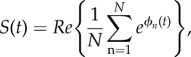2.14

where the generalized phase (including both precession and relaxation) was updated every time step using:

2.15

and

2.16

where γ is the hydrogen proton precession frequency, j the imaginary unit and

2.17

with the magnetic field homogeneity computed above, and is the field homogeneity introduced by the spatial gradient.

This procedure is repeated at each desired time point during the functional activation. The relative signal changes were computed by comparing the signal obtained at each time point to the signal obtained at t = 0 and converted to a per cent change.

3. Results

(a). BOLD-cerebral blood flow, isometabolic contours and optimization of the free parameters of the Davis model

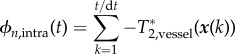
The BOLD responses simulated for each of our 72 simulations (three arterial dilations ×4 CMRO₂ increases ×6 VANs) are illustrated in figure 3 as a function of CBF increase. Each BOLD response was normalized by the maximal BOLD response (M) on the plot. Each symbol corresponds to simulations performed on the same VAN model, and each colour corresponds to different CMRO₂ increases. Note that the same level of arterial dilation (10%, 20% and 30%) produces different levels of CBF increases in individual animals because of different vascular resistances owing to different vessel diameters and network topologies. Running the optimization procedure, we find that the optimal values for the two free parameters of the Davis model (i.e. the values that minimize the error (MSE) between the true simulated microscopic change in CMRO₂ and the recovered macroscopic change in CMRO₂) are α =−0.05 and β = 0.98 for B₀ = 3 T and TE = 30 ms. The solid lines in figure 3 illustrate the theoretical BOLD-CBF responses obtained from the Davis model with α =−0.05 and β = 0.98 for different CMRO₂ increases also termed BOLD-CBF isometabolic contour plots [8].

Figure 3.

BOLD-CBF isometabolic contour plots illustrating the 72 simulations (three dilations ×4 CMRO₂ increases ×6 VANs). Each symbol represents an individual animal or VAN. Different levels of CMRO₂ increases are illustrated by different colours. It is to note that the same level of arterial dilation (10%, 20% and 30%) produces different levels of CBF increase for each animal. The values shown (α =−0.05 and β = 0.98) are the ones that minimized the mean square error between the simulated rCMRO₂ and the recovered macroscopic rCMRO₂ using the Davis model. Solid lines illustrate the theoretical BOLD signal from the Davis model for (α =−0.05 and β = 0.98), i.e. the best fit of the Davis model to the simulated data (individual symbols).

(b). Accuracy of the Davis model to recover changes in cerebral metabolic rate of oxygen

A scatter plot of the simulated versus recovered change in CMRO₂ is illustrated in figure 4a when the optimal values for α and β are used (α = −0.05 and β = 0.98). We see that the slope of the best linear fit to the scatter plot is 0.96, which is very close to unity. This indicates that the Davis model with the optimized parameters recovers changes in CMRO₂ with very negligible bias on average. However, we also see from figure 4a that the dispersion of the scatter plot lies in-between ±5%, from which we can deduce that the uncertainty on the recovered rCMRO₂ is about 5% without considering experimental noise. Note that this 5% is an absolute per cent change, i.e. a 15% increase should be interpreted as an increase between 10% and 20%. However, this uncertainty should be interpreted as the intrinsic accuracy of the Davis model only, reflecting the effect of physiological and anatomical variability that the Davis model does not include. In addition, random noise in in vivo experiments must also be considered in practical applications. In particular, the additional noise from the ASL measurement of CBF [5] is a major consideration.

Figure 4.

Validation and optimization of the Davis model. (a) Optimization of the free parameter α and β. The values shown (α =−0.05 and β = 0.98) are the ones that minimized the mean-squared error between the simulated microscopic rCMRO₂ and the recovered macroscopic rCMRO₂. The values for each individual simulations are displayed on a scatter plot of the recovered rCMRO₂ versus the simulated rCMRO₂. (b) Scatter plot of recovered versus simulated rCMRO₂ by using the values for the free parameters proposed by Griffeth et al. [28]. (c) Scatter plot of recovered versus simulated rCMRO₂ by using the values for the free parameters originally proposed by Davis et al. [7]. (d) Mean-squared error between the recovered and the simulated rCMRO₂ for three different sets of the free parameters: our new optimized values, Griffeth et al. [28] and Davis et al. [7]. (e) Plot of the BOLD responses obtained from different increases in CBF with each of the three sets of values for the free parameter. A flow-metabolic coupling ratio of 2 was assumed. (f) Same as (e) but with flow-metabolic coupling of 3 assumed.

For comparison, we also tested the accuracy of the Davis model to recover changes in CMRO₂, using values previously reported for α and β. The scatter plot obtained, using the values of α = 0.10 and β = 0.90 previously computed from Griffeth et al. [28], is shown in figure 4b. The slope of the best linear fit is 0.78, indicating that the Davis model with α = 0.10 and β = 0.90 tends to systematically underestimate changes in CMRO₂ by a relative 22% (i.e. that a 20% measured increase should be interpreted as a 24.4% increase). Finally, the scatter plot obtained using the original values of α = 0.38 and β = 1.5 is shown in figure 4c. The slope of the best linear fit is 0.66 indicating that the Davis model with α = 0.38 and β = 1.5 underestimates changes in CMRO₂ by a relative 34% at 3 T (i.e. that a 20% measured increase should be interpreted as a 26.8% increase). Note that the data in the original Davis et al. work [7] were acquired at 1.5 T and, therefore, the uncertainty obtained here is not applicable to their work. A quantitative comparison of the performance obtained using the three sets of free parameters is shown in figure 4d, where the MSEs between the simulated and the recovered changes in CMRO₂ are compared. We observe that the new values of α = −0.05 and β = 0.98 reduce the MSE by 25% compared with using α = 0.10 and β = 0.90.

We emphasize that because α and β are no longer treated as physical parameters, but rather as free parameters, they no longer correspond to the physiological effect they were meant to model. Therefore, the negative value of the parameter α has no special physical meaning and should not be interpreted as a negative compliance, because α does not reflect vessel compliance anymore. The free parameters α and β are now fitting parameters that can take any positive or negative values. To avoid any confusion and to clarify this point, the traces of the BOLD responses for the different sets of free parameters are superimposed in figure 4e and f for a flow-metabolic coupling ratio of 2 and 3, respectively. We see from these traces that the optimized value of α = −0.05 and β = 0.98 simply predicts a stronger BOLD response compared with the one predicted with α = 0.10 and β = 0.90, without any non-physical macroscopic behaviour. Further discussion on the meaning of these new values for α and β is provided in the Discussion section.

(c). Variation with B-field strength

One of the key features of our simulation approach is that the BOLD signal can be predicted for any B-field strength. It was therefore possible to repeat the entire optimization procedure for different magnet strengths ranging from 1.5 to 14 T. The optimal values for α and β in each case are shown in table 1 as well as the TE value used in the simulations. The fact that α varies for different values of the external B-field emphasizes the point that α does not reflect vessel compliance anymore (or any purely physiological parameters that should not vary with B-field) but rather multiple physical and physiological effects.

Table 1.

Optimal values for free parameters α and β for different B₀-field strengths.

B-field (T)	TE (ms)	α	β
1.5	45	−0.09	0.30
3.0	30	−0.05	0.98
4.7	30	0.30	1.15
7.0	22	0.25	0.67
9.4	22	0.20	0.76
11.7	19	0.18	0.82
14.0	16	0.17	0.79

(d). Values are robust to different levels of venous compliance

One of the limitations of our approach is the possibility that the craniotomy, even if done with the most careful considerations, alters venous dilation. Work done with a thin-skull procedure [32,56], a less invasive approach, has reported larger venous dilation following forepaw stimulus compared with a standard craniotomy. This potential pitfall can be handled in our VAN model by forcing the dilation of the veins to be larger. In this work, we tested the robustness of our optimization procedure by simulating BOLD responses when the veins were forced to dilate according to a Grubb relationship with an exponent of 0.38. Then, the optimization procedure for α and β was repeated, and the new values of α = −0.02 and β = 0.79 were obtained. These results are shown in figure 5a. We also tested the recovery of rCMRO₂ on these same data generated with the forced venous dilation but using instead the set of optimal values obtained without forcing a larger venous dilation (α = −0.05 and β = 0.98). As shown in figure 5b, we see that using α = −0.05 and β = 0.98 performs almost as well as the newly optimized parameters (α = −0.02 and β = 0.79) indicating that our initial optimization values are still valid even if the veins dilate more than our original negligible dilation. Although the slope of the best linear fit is a little closer to unity with α = −0.05 and β = 0.98 compared with α = −0.02 and β = 0.79 (0.99 compared with 0.95), the MSE is a little lower with α = −0.02 and β = 0.79 as shown in figure 5c, as expected from an optimization procedure.

Figure 5.

Effect of a larger venous dilation. (a) Optimization of the free parameter α and β for VAN simulations in which the veins were forced to dilate according to a Grubb exponent of 0.38. In this case, the optimal values obtained were α = −0.02 and β = 0.79. (b) Scatter plot of the recovered rCMRO₂ versus the simulated rCMRO₂ by simulating the BOLD response with the forced venous dilation but by using the optimal values computed with negligible venous dilation (i.e. α = −0.05 and β = 0.98) rather than the ones optimized for the large venous dilation (α = −0.02 and β = 0.79). (c) Mean-squared error between the simulated and the recovered rCMRO₂ obtained using each set of free parameters. In each case, the BOLD response was simulated by forcing a large venous dilation in the VAN. The only difference is the value used as free parameters in the Davis model.

(e). Impact of different echo times

When BOLD and ASL signals are acquired simultaneously, the BOLD signal is obtained from the control images of the ASL sequence. The optimal TE for ASL is generally lower than the optimal TE for BOLD [11,57–59]. As a trade-off, the TE used in combined BOLD-ASL acquisitions is generally lower than the usual TE = 30 ms. Therefore, we also simulated the BOLD response from our VAN simulations with TE = 13 ms at 3 T [59], and the results for the optimal values of the free parameters are presented in table 2. We found that in this case, α = −0.02 and β = 0.56 minimized the mean-squared error between the simulated and the recovered rCMRO₂.

Table 2.

Optimal values for free parameters α and β for different TEs at 3 T.

TE=30 ms		TE=13 ms
α	β	α	β
−0.05	0.98	−0.02	0.56

(f). The simple heuristic BOLD model performs as well as the regular Davis model

We also tested the accuracy of the simplified heuristic BOLD model [29] presented in equation (2.2) to recover changes in CMRO₂. As shown in figure 6a, our optimization adapted for the heuristic model computed α_v = −0.05 as the optimal value of the sole free parameter. We also observe a negligible bias on the recovery of rCMRO₂ with a slope of the best linear fit of 0.95 which is very close to unity. For comparison, we have reproduced the scatter plot for the Davis model (figure 4a) with the optimized parameters in figure 6b. The performance of the two optimized models is compared in figure 6c by showing the MSEs between the simulated and the recovered changes in CMRO₂. We see that both models perform very well, but still the Davis model performs a little better compared with the simplified heuristic BOLD model. However, this improvement is mostly negligible. For completeness, the optimal value for α_v was computed for different magnet strengths, and results are displayed in table 3.

Figure 6.

Accuracy of a simplified heuristic BOLD model (Griffeth [29]). (a) Optimization of the sole free parameter (α_v = −0.05) of the heuristic model using the same procedure illustrated in figure 1. (b) Replication of figure 4b for comparison purpose. (c) Mean-squared error between the simulated rCMRO₂ and the recovered rCMRO₂ using the Davis model with our new optimized parameters (α = −0.05 and β = 0.98) and the heuristic model with (α_v = −0.05).

Table 3.

Optimal values for free parameters α_v for different B₀-field strengths.

B-field (T)	TE (ms)	αv
1.5	45	−0.42
3.0	30	−0.05
3.0	13	−0.08
4.7	30	0.29
7.0	22	0.39
9.4	22	0.29
11.7	19	0.24
14.0	16	0.20

4. Discussion

In this work, we used our recently developed microscopic VAN model in mice as a ground truth simulator to test the accuracy of macroscopic, lumped-parameter BOLD models to accurately recover evoked changes in CMRO₂. By measuring microscopic cortical physiology with quantitative two-photon microscopy, we removed all ambiguities in the microscopic physiological parameters, allowing for a bottom-up validation of hypercapnic-calibrated fMRI. Our approach allowed us to optimize the two free parameters of the macroscopic BOLD model to better fit the microscopic data and therefore providing a more accurate recovery of CMRO₂.

(a). Microscopic validation of calibrated functional magnetic resonance imaging

The validity of using simplified biophysical models of the BOLD signal to quantify CMRO₂ changes has not been firmly established from a bottom-up perspective. However, the CMRO₂ values obtained have been compared with other top-down approaches such as PET [60]. There is a general consistency in the results from fMRI and PET studies of the ratio of CBF changes to CMRO₂ changes (termed ‘n’) observed during brain activation [3,60]. It is to note that this ratio varies between 2 and 4 and depends strongly on the brain region studied [3]. The original observation of the CBF/CMRO₂ mismatch by Fox & Raichle [61] is one of the largest values of n found (approx. 6), but later PET studies found n ∼ 2 in other brain regions (reviewed in [3]). There is a trend in the literature for motor/somatosensory data to have the highest values of n, basal ganglia to have the lowest values and visual areas to lie in the middle. The n ratio varies also with the frequency of the stimulus because CBF does not monotonically increase with stimulus frequency but rather peaks and then decreases as the frequency increases [60]. Therefore, careful consideration must be taken into account when comparing n values in the literature, but there is generally good agreement between fMRI and PET when all these sources of variation are considered [60,62].

Calibrated fMRI has also been compared with multimodal optical-fMRI fusion imaging [63] at the single-subject level [59]. In this case, the n values obtained over the motor cortex were similar between the two methods [59]. The value of the calibration constants M was also obtained separately from optical-fMRI fusion and was compared against the ones obtained from the hypercapnic scan for individual subjects. An intersubject correlation coefficient of R = 0.87 was obtained between the two methods for the M values [59].

Even if the BOLD response has a complex biophysical origin [53,64], a very simple model such as the Davis model is sufficient to recover changes in CMRO₂. The reason for this surprising accuracy resides in the form of the Davis model, consisting of two free parameters and a calibration constant. Most of the unknown physiological information such as baseline venous blood-to-tissue fraction (V₀), baseline OEF (E₀) and the unknown physical information such as the frequency offset of water at the outer surface of a magnetized vessel (ν₀), are lumped into the calibration constant M, which is estimated from the hypercapnic trial. The calibration experiment plays a crucial role here, because it allows M to be a more general parameter. It is not required to be equal to 4.3 ν₀ V₀ E₀ TE as in the original derivation of the Davis model, where only extravascular signal changes were considered. In these simulations based on the VAN model, M emerges only as an empirical value based on simulations of the hypercapnia experiment, so it is free to capture additional scaling effects owing, for example, to intravascular signal changes. Moreover, a sensitivity analysis has revealed that the sensitivity of the recovered change in CMRO₂ to α and β is very low because the same values are used in both the calibration part (estimation of M) and the subsequent estimation of rCMRO₂, which means that a wrong assumption of α or β is partially cancelled out [7].

Both the PET [60] and the multimodal optical-fMRI fusion [59] studies provided what we called top-down validations. The alternative is a bottom-up validation, which shows that a more detailed model based on underlying first principles converges to a simpler model, therefore validating the formulation of the simpler model. We have achieved this bottom-up validation in our work by using a real vascular geometry, using experimentally measured oxygen distributions throughout the vascular network [27], and considering the most recent two-photon measurements of vessel dilation [21,32]. The consistency of our results with the multi-compartment modelling from Griffeth [28] increases confidence in our bottom-up modelling approach to validate calibrated fMRI.

(b). Impact of no venous dilation and lower capillary oxygenation on calibrated functional magnetic resonance imaging

First, our VAN model (as well as the four-compartment model of Griffeth et al. [28]) takes into account the fact that a large fraction of the volume increase during functional activation occurs in the arterial compartment. This means that the value of the parameter α assumed in early studies was too high. However, as mentioned above, an incorrect assumption of α only slightly affects the recovery of rCMRO₂ because most of the error is cancelled out by assuming the same wrong α value during the calibration procedure [7]. Second, our VAN simulations take into account a feature of oxygen extraction in the brain, i.e. that a significant portion (50% in anaesthetized animals) of the oxygen leaves the vasculature from the arterioles before the capillaries. Retrospectively, we could have expected that this feature of cerebral oxygen extraction does not affect the accuracy of calibrated BOLD to recover changes in CMRO₂. The reason is that venous SO₂ depends on the total arterial and capillary OEF, and not the individual weight of these two compartments to the total OEF. Whether the oxygen is extracted before or during capillary passage only affects capillary SO₂, which was already known to have a very minor effect in gradient-echo BOLD that originates mostly from the venous compartment [17,53,65].

(c). More on the optimal α and β values

Although the Davis model was originally designed with two independent parameters, what shows up in its analytical expression (equation (2.1)) is α – β. Because α and β are treated as fitting parameters in our optimization procedure, it is justified to lump α – β into a single parameter θ = α – β and to compare the optimized value of θ and β with their original values. In the original Davis model, α = 0.38 and β = 1.5, so θ = −1.12. The negative value of θ is justified for the equation to produce a larger BOLD response when the CBF response is larger, because δBOLD is proportional to 1 – rCBF^θ for constant CMRO₂. With our optimized values of α = −0.05 and β = 0.98, the new optimized value of θ is −1.03, which is very close to the original θ = −1.12 value and, therefore, the Davis model with the new optimized parameters produces very similar BOLD responses compared with the Davis model with the original value of the parameters. This is illustrated in figure 4e,f.

Moreover, we emphasize that because the optimal value for α depends on the strength of the magnet (table 1), α cannot reflect a purely physiological phenomenon such as vessel compliance anymore. The parameter α is now treated as a fitting parameter that reflects several physical (B-field-dependent) and physiological effects. Therefore, its negative value does not reflect a physiological improbability.

(d). Linking microscopic to macroscopic parameters

As mentioned above, the results presented in this work indicated that the macroscopic parameter α of the Davis model cannot reflect a purely physiological phenomenon such as microscopic vascular compliance. Although the Davis model was not derived to recover microscopic vascular compliance, our results indicate that this model could not be used to infer vascular compliance in any way. If one were to measure α rather than assume its value, the value recovered would not reflect purely vascular compliance but rather several physical and physiological effects. Therefore, more detailed models are required to link microscopic physiological parameters to macroscopic physiological parameters that can be measured routinely in fMRI studies.

The theoretical framework developed in Gagnon et al. [17] and used in this work will allow the derivation of more simplified models that perform this task, i.e. that allow the inference of microscopic physiology from macroscopic measurements. This will allow the validation and refinement of integrative models of macroscopic signals to provide quantitative information about microvascular physiology. These validated models could then be used routinely in human studies where only macroscopic measurements are currently available.

(e). Quantitative physiological functional magnetic resonance imaging: other methods

Standard hypercapnic-calibrated fMRI with the Davis model permits the recovery of changes in CMRO₂ during a functional task. This parameter is very useful, because it provides a more direct measurement of the variation in neuronal activity during the functional task. However, hypercapnic-calibrated fMRI, as originally proposed by Davis et al. [7], does not provide a measurement of baseline or resting CMRO₂, which is a more clinically relevant parameter. Several fMRI methods have been developed to recover baseline CMRO₂. One of these methods is an extension of calibrated fMRI with both hypercapnia and hyperoxia [14–16]. This method has recently been refined using a compartmental BOLD model [66]. In future work, the bottom-up approach presented in this work could be used to validate and potentially refine the estimation of baseline CMRO₂ with the extended hyperoxia–hypercapnia-calibrated fMRI method. Another method proposed to measure baseline OEF is termed q-BOLD [67,68]. In q-BOLD, a parametric macroscopic model (different from the Davis model) of the baseline T*₂ signal is used to estimate baseline OEF from baseline BOLD acquisition and a subsequent baseline ASL acquisition can be used to compute baseline CMRO₂. Our bottom-up approach could be used also to validate and potentially refine the q-BOLD approach.

Finally, in this work, we simulated the BOLD response with a Monte Carlo approach, whereas the CBF value was assumed to be perfectly known. In practice, the relation between the ASL signal measured and the CBF value is linear [35] and, therefore, there is very little systematic bias in the estimated rCBF from ASL. However, the procedure is noisy because of the subtraction of two scans and because of the difficulty of efficiently tagging spins. In future work, our Monte Carlo approach could be modified to also simulate the ASL signal, making our bottom-up approach more realistic and more versatile by allowing modifications for different ASL sequence parameters.

5. Conclusion

In this work, we simulated the calibrated fMRI approach from first principles, using real microvascular measurements and simulations of cortical physiology. Our method enabled us to validate calibrated fMRI from the microscopic point of view and to optimize the free parameters of the macroscopic biophysical model assumed (i.e. the Davis model). We found that by using α = −0.05 and β = 0.98 in the computation of both M and rCMRO₂, the error in the estimated rCMRO₂ is ±5% absolute. We found that the optimized values of the free parameters are robust to different vascular compliances of the venous compartment. Finally, we found that the simple heuristic BOLD model has almost the same accuracy as the Davis model to recover changes in CMRO₂ from combined BOLD and ASL measurements.

Data Accessibility

All the data used in this manuscript are available upon request by email to the corresponding author.

Authors' contributions

L.G., R.B.B., A.M.D., A.D. and D.A.B designed the study. S.S. collected the two-photon data. L.G., F.L. and P.P. designed the Monte Carlo code for BOLD simulations with inputs from R.B.B. All authors contributed to the text of the manuscript.

Competing interests

The authors declare no competing interest.

Funding

This work was supported by NIH grants nos. P41RR14075, R01NS057476, R00NS067050, R01NS057198 and R01EB000790, American Heart Association grant no. 11SDG7600037, and the Advanced Multimodal NeuroImaging Training Program (R90DA023427 to L.G.).

References

- 1.Logothetis NK, Pauls J, Augath M, Trinath T, Oeltermann A. 2001. Neurophysiological investigation of the basis of the fMRI signal. Nature 412, 150–157. ( 10.1038/35084005) [DOI] [PubMed] [Google Scholar]
- 2.Lin A-L, Fox PT, Hardies J, Duong TQ, Gao J-H. 2010. Nonlinear coupling between cerebral blood flow, oxygen consumption, and ATP production in human visual cortex. Proc. Natl Acad. Sci. USA 107, 8446–8451. ( 10.1073/pnas.0909711107) [DOI] [PMC free article] [PubMed] [Google Scholar]
- 3.Buxton RB. 2010. Interpreting oxygenation-based neuroimaging signals: the importance and the challenge of understanding brain oxygen metabolism. Front. Neuroenerg. 2, 8–8. ( 10.3389/fnene.2010.00008) [DOI] [PMC free article] [PubMed] [Google Scholar]
- 4.Huppert TJ, Jones PB, Devor A, Dunn AK, Teng IC, Dale AM, Boas DA. 2009. Sensitivity of neural-hemodynamic coupling to alterations in cerebral blood flow during hypercapnia. J. Biomed. Opt. 14, 044038–044038-16. ( 10.1117/1.3210779) [DOI] [PMC free article] [PubMed] [Google Scholar]
- 5.Hoge RD. 2012. Calibrated FMRI. Neuroimage 62, 930–937. ( 10.1016/j.neuroimage.2012.02.022) [DOI] [PubMed] [Google Scholar]
- 6.Pike GB. 2012. Quantitative functional MRI: concepts, issues and future challenges. Neuroimage 62, 1234–1240. ( 10.1016/j.neuroimage.2011.10.046) [DOI] [PubMed] [Google Scholar]
- 7.Davis TL, Kwong KK, Weisskoff RM, Rosen BR. 1998. Calibrated functional MRI: mapping the dynamics of oxidative metabolism. Proc. Natl Acad. Sci. USA 95, 1834–1839. ( 10.1073/pnas.95.4.1834) [DOI] [PMC free article] [PubMed] [Google Scholar]
- 8.Hoge RD, Atkinson J, Gill B, Crelier GR, Marrett S, Pike GB. 1999. Investigation of BOLD signal dependence on cerebral blood flow and oxygen consumption: the deoxyhemoglobin dilution model. Magn. Reson. Med. 42, 849–863. ( 10.1002/(SICI)1522-2594(199911)42:5%3C849::AID-MRM4%3E3.0.CO;2-Z) [DOI] [PubMed] [Google Scholar]
- 9.Grubb RL, Raichle ME, Eichling JO, Ter-Pogossian MM. 1974. The effects of changes in PaCO2 on cerebral blood volume, blood flow, and vascular mean transit time. Stroke 5, 630–639. ( 10.1161/01.STR.5.5.630) [DOI] [PubMed] [Google Scholar]
- 10.Boxerman JL, Hamberg LM, Rosen BR, Weisskoff RM. 1995. MR contrast due to intravascular magnetic susceptibility perturbations. Magn. Reson. Med. 34, 555–566. ( 10.1002/mrm.1910340412) [DOI] [PubMed] [Google Scholar]
- 11.Gauthier CJ, Madjar C, Tancredi FB, Stefanovic B, Hoge RD. 2011. Elimination of visually evoked BOLD responses during carbogen inhalation: implications for calibrated MRI. Neuroimage 54, 1001–1011. ( 10.1016/j.neuroimage.2010.09.059) [DOI] [PubMed] [Google Scholar]
- 12.Blockley NP, Griffeth VEM, Simon AB, Dubowitz DJ, Buxton RB. 2015. Calibrating the BOLD response without administering gases: comparison of hypercapnia calibration with calibration using an asymmetric spin echo. Neuroimage 104, 423–429. ( 10.1016/j.neuroimage.2014.09.061) [DOI] [PMC free article] [PubMed] [Google Scholar]
- 13.Blockley NP, Griffeth VEM, Buxton RB. 2011. A general analysis of calibrated BOLD methodology for measuring CMRO2 responses: Comparison of a new approach with existing methods. Neuroimage 60, 279–289. ( 10.1016/j.neuroimage.2011.11.081) [DOI] [PMC free article] [PubMed] [Google Scholar]
- 14.Gauthier CJ, Hoge RD. 2012. A generalized procedure for calibrated MRI incorporating hyperoxia and hypercapnia. Hum. Brain Mapp. 34, 1053–1069. ( 10.1002/hbm.21495) [DOI] [PMC free article] [PubMed] [Google Scholar]
- 15.Gauthier CJC, Hoge RD. 2012. Magnetic resonance imaging of resting OEF and CMRO2 using a generalized calibration model for hypercapnia and hyperoxia. Neuroimage 60, 14 ( 10.1016/j.neuroimage.2011.12.056) [DOI] [PubMed] [Google Scholar]
- 16.Gauthier CJ, Desjardins-Crépeau L, Madjar C, Bherer L, Hoge RD. 2012. Absolute quantification of resting oxygen metabolism and metabolic reactivity during functional activation using QUO2 MRI. Neuroimage 63, 1353–1363. ( 10.1016/j.neuroimage.2012.07.065) [DOI] [PubMed] [Google Scholar]
- 17.Gagnon L, et al. 2015. Quantifying the microvascular origin of BOLD-fMRI from first principles with two-photon microscopy and an oxygen-sensitive nanoprobe. J. Neurosci. 35, 3663–3675. ( 10.1523/JNEUROSCI.3555-14.2015) [DOI] [PMC free article] [PubMed] [Google Scholar]
- 18.Hillman EMC, Devor A, Bouchard MB, Dunn AK, Krauss GW, Skoch J, Bacskai BJ, Dale AM, Boas DA. 2007. Depth-resolved optical imaging and microscopy of vascular compartment dynamics during somatosensory stimulation. Neuroimage 35, 89–104. ( 10.1016/j.neuroimage.2006.11.032) [DOI] [PMC free article] [PubMed] [Google Scholar]
- 19.Devor A, et al. 2008. Stimulus-induced changes in blood flow and 2-deoxyglucose uptake dissociate in ipsilateral somatosensory cortex. J. Neurosci. 28, 14 347–14 357. ( 10.1523/JNEUROSCI.4307-08.2008) [DOI] [PMC free article] [PubMed] [Google Scholar]
- 20.Devor A, et al. 2007. Suppressed neuronal activity and concurrent arteriolar vasoconstriction may explain negative blood oxygenation level-dependent signal. J. Neurosci. 27, 4452–4459. ( 10.1523/JNEUROSCI.0134-07.2007) [DOI] [PMC free article] [PubMed] [Google Scholar]
- 21.Tian P, et al. 2010. Cortical depth-specific microvascular dilation underlies laminar differences in blood oxygenation level-dependent functional MRI signal. Proc. Natl Acad. Sci. USA 107, 15 246–15 251. ( 10.1073/pnas.1006735107) [DOI] [PMC free article] [PubMed] [Google Scholar]
- 22.Devor A, Dunn AK, Andermann ML, Ulbert I, Boas DA, Dale AM. 2003. Coupling of total hemoglobin concentration, oxygenation, and neural activity in rat somatosensory cortex. Neuron 39, 353–359. ( 10.1016/S0896-6273(03)00403-3) [DOI] [PubMed] [Google Scholar]
- 23.Srinivasan VJ, Sakadžić S, Gorczynska I, Ruvinskaya S, Wu W, Fujimoto JG, Boas DA. 2010. Quantitative cerebral blood flow with optical coherence tomography. Opt. Express. 18, 2477–2494. ( 10.1364/OE.18.002477) [DOI] [PMC free article] [PubMed] [Google Scholar]
- 24.Srinivasan VJ, et al. 2011. Optical coherence tomography for the quantitative study of cerebrovascular physiology. J. Cereb. Blood Flow Metab. 31, 1339–1345. ( 10.1038/jcbfm.2011.19) [DOI] [PMC free article] [PubMed] [Google Scholar]
- 25.Sakadžić S, et al. 2010. Two-photon high-resolution measurement of partial pressure of oxygen in cerebral vasculature and tissue. Nat. Methods 7, 755–759. ( 10.1038/nmeth.1490) [DOI] [PMC free article] [PubMed] [Google Scholar]
- 26.Devor AA, et al. 2011. ‘Overshoot’ of O2 is required to maintain baseline tissue oxygenation at locations distal to blood vessels. J. Neurosci. 31, 13 676–13 681. ( 10.1523/JNEUROSCI.1968-11.2011) [DOI] [PMC free article] [PubMed] [Google Scholar]
- 27.Sakadžić S, et al. 2014. Large arteriolar component of oxygen delivery implies a safe margin of oxygen supply to cerebral tissue. Nat. Commun. 5, 5734 ( 10.1038/ncomms6734) [DOI] [PMC free article] [PubMed] [Google Scholar]
- 28.Griffeth VEM, Buxton RB. 2011. A theoretical framework for estimating cerebral oxygen metabolism changes using the calibrated-BOLD method: modeling the effects of blood volume distribution, hematocrit, oxygen extraction fraction, and tissue signal properties on the BOLD signal. Neuroimage 58, 198–212. ( 10.1016/j.neuroimage.2011.05.077) [DOI] [PMC free article] [PubMed] [Google Scholar]
- 29.Griffeth VEM, Blockley NP, Simon AB, Buxton RB. 2013. A new functional MRI approach for investigating modulations of brain oxygen metabolism. PLoS ONE 8, e68122 ( 10.1371/journal.pone.0068122) [DOI] [PMC free article] [PubMed] [Google Scholar]
- 30.Tancredi FB, Hoge RD. 2013. Comparison of cerebral vascular reactivity measures obtained using breath-holding and CO2 inhalation. J. Cereb. Blood Flow Metab. 33, 1066–1074. ( 10.1038/jcbfm.2013.48) [DOI] [PMC free article] [PubMed] [Google Scholar]
- 31.Chen JJ, Pike GB. 2010. Global cerebral oxidative metabolism during hypercapnia and hypocapnia in humans: implications for BOLD fMRI. J. Cereb. Blood Flow Metab. 30, 1094–1099. ( 10.1038/jcbfm.2010.42) [DOI] [PMC free article] [PubMed] [Google Scholar]
- 32.Drew P, Shih AY, Kleinfeld D. 2011. Fluctuating and sensory-induced vasodynamics in rodent cortex extend arteriole capacity. Proc. Natl Acad. Sci. USA 108, 8473–8478. ( 10.1073/pnas.1100428108) [DOI] [PMC free article] [PubMed] [Google Scholar]
- 33.Duling BR, Berne RM. 1970. Longitudinal gradients in periarteriolar oxygen tension. A possible mechanism for the participation of oxygen in local regulation of blood flow. Circ. Res. 27, 669–678. ( 10.1161/01.RES.27.5.669) [DOI] [PubMed] [Google Scholar]
- 34.Stamler JS, Jia L, Eu JP, McMahon TJ, Demchenko IT, Bonaventura J, Gernert K, Piantadosi CA. 1997. Blood flow regulation by S-nitrosohemoglobin in the physiological oxygen gradient. Science 276, 2034–2037. ( 10.1126/science.276.5321.2034) [DOI] [PubMed] [Google Scholar]
- 35.Buxton RB, Frank LR, Wong EC, Siewert B, Warach S, Edelman RR. 1998. A general kinetic model for quantitative perfusion imaging with arterial spin labeling. Magn. Reson. Med. 40, 383–396. ( 10.1002/mrm.1910400308) [DOI] [PubMed] [Google Scholar]
- 36.Finikova OS, Lebedev AY, Aprelev A, Troxler T, Gao F, Garnacho C, Muro S, Hochstrasser RM, Vinogradov SA. 2008. Oxygen microscopy by two-photon-excited phosphorescence. Chemphyschem 9, 1673–1679. ( 10.1002/cphc.200800296) [DOI] [PMC free article] [PubMed] [Google Scholar]
- 37.Parpaleix A, Houssen YG, Charpak S.. 2013. Imaging local neuronal activity by monitoring PO2 transients in capillaries. Nat. Med. 19, 241–246. ( 10.1038/nm.3059) [DOI] [PubMed] [Google Scholar]
- 38.Uchida K, Reilly MP, Asakura T.. 1998. Molecular stability and function of mouse hemoglobins. Zool. Sci. 15, 703–706. ( 10.2108/zsj.15.703) [DOI] [Google Scholar]
- 39.Gagnon L, Sakadžić S, Lesage F, Mandeville ET, Fang Q, Yaseen MA, Boas DA. 2015. Multimodal reconstruction of microvascular-flow distributions using combined two-photon microscopy and Doppler optical coherence tomography. Neurophoton 2, 015008 ( 10.1117/1.NPh.2.1.015008) [DOI] [PMC free article] [PubMed] [Google Scholar]
- 40.Wehrl HF, Judenhofer MS, Maier FC, Martirosian P, Reischl G, Schick F, Pichler BJ. 2010. Simultaneous assessment of perfusion with [15O] water PET and arterial spin labeling MR using a hybrid PET/MR device. ISMRM 18, 715. [Google Scholar]
- 41.Zheng B, Lee PTH, Golay X.. 2010. High-sensitivity cerebral perfusion mapping in mice by kbGRASE-FAIR at 9.4T. NMR Biomed. 23, 1061–1070. ( 10.1002/nbm.1533) [DOI] [PubMed] [Google Scholar]
- 42.Ito H, Kanno I, Fukuda H.. 2005. Human cerebral circulation: positron emission tomography studies. Ann. Nucl. Med. 19, 65–74. ( 10.1007/BF03027383) [DOI] [PubMed] [Google Scholar]
- 43.Lorthois S, Cassot F, Lauwers F.. 2011. Simulation study of brain blood flow regulation by intra-cortical arterioles in an anatomically accurate large human vascular network. Part II: flow variations induced by global or localized modifications of arteriolar diameters. Neuroimage 54, 2840–2853. ( 10.1016/j.neuroimage.2010.10.040) [DOI] [PubMed] [Google Scholar]
- 44.Lorthois S, Cassot F, Lauwers F.. 2011. Simulation study of brain blood flow regulation by intra-cortical arterioles in an anatomically accurate large human vascular network: part I: methodology and baseline flow. Neuroimage 54, 1031–1042. ( 10.1016/j.neuroimage.2010.09.032) [DOI] [PubMed] [Google Scholar]
- 45.Pries AR, Secomb TW, Gaehtgens P, Gross JF. 1990. Blood flow in microvascular networks. Experiments and simulation. Circ. Res. 67, 826–834. ( 10.1161/01.RES.67.4.826) [DOI] [PubMed] [Google Scholar]
- 46.Lipowsky HH. 2005. Microvascular Rheology and Hemodynamics. UMIC 12, 5–15. ( 10.1080/10739680590894966) [DOI] [PubMed] [Google Scholar]
- 47.Boas DA, Jones SR, Devor A, Huppert TJ, Dale AM. 2008. A vascular anatomical network model of the spatio-temporal response to brain activation. Neuroimage 40, 1116–1129. ( 10.1016/j.neuroimage.2007.12.061) [DOI] [PMC free article] [PubMed] [Google Scholar]
- 48.Fang Q, Sakadžić S, Ruvinskaya L, Devor A, Dale AM, Boas DA. 2008. Oxygen advection and diffusion in a three-dimensional vascular anatomical network. Opt. Express. 16, 17 530–17 541. ( 10.1364/OE.16.017530) [DOI] [PMC free article] [PubMed] [Google Scholar]
- 49.Yablonskiy DA, Haacke EM. 1994. Theory of NMR signal behavior in magnetically inhomogeneous tissues: the static dephasing regime. Magn. Reson. Med. 32, 749–763. ( 10.1002/mrm.1910320610) [DOI] [PubMed] [Google Scholar]
- 50.Koch KM, Papademetris X, Rothman DL, de Graaf RA. 2006. Rapid calculations of susceptibility-induced magnetostatic field perturbations for in vivo magnetic resonance. Phys. Med. Biol. 51, 6381–6402. ( 10.1088/0031-9155/51/24/007) [DOI] [PubMed] [Google Scholar]
- 51.Pathak AP, Ward BD, Schmainda KM. 2008. A novel technique for modeling susceptibility-based contrast mechanisms for arbitrary microvascular geometries: the finite perturber method. Neuroimage 40, 1130–1143. ( 10.1016/j.neuroimage.2008.01.022) [DOI] [PMC free article] [PubMed] [Google Scholar]
- 52.Christen T, Zaharchuk G, Pannetier N, Serduc R, Joudiou N, Vial J-C, Rémy C, Barbier EL. 2011. Quantitative MR estimates of blood oxygenation based on T2*: a numerical study of the impact of model assumptions. Magn. Reson. Med. 67, 1458–1468. ( 10.1002/mrm.23094) [DOI] [PubMed] [Google Scholar]
- 53.Uludağ K, Müller-Bierl B, Uğurbil K.. 2009. An integrative model for neuronal activity-induced signal changes for gradient and spin echo functional imaging. Neuroimage 48, 150–165. ( 10.1016/j.neuroimage.2009.05.051) [DOI] [PubMed] [Google Scholar]
- 54.Boxerman JL, Bandettini PA, Kwong KK, Baker JR, Davis TL, Rosen BR, Weisskoff RM. 1995. The intravascular contribution to fMRI signal change: Monte Carlo modeling and diffusion-weighted studies in vivo. Magn. Reson. Med. 34, 4–10. ( 10.1002/mrm.1910340103) [DOI] [PubMed] [Google Scholar]
- 55.Martindale J, Kennerley AJ, Johnston D, Zheng Y, Mayhew JE. 2008. Theory and generalization of Monte Carlo models of the BOLD signal source. Magn. Reson. Med. 59, 607–618. ( 10.1002/mrm.21512) [DOI] [PubMed] [Google Scholar]
- 56.Drew PJ, Shih AY, Driscoll JD, Knutsen PM, Blinder P, Davalos D, Akassoglou K, Tsai PS, Kleinfeld D. 2010. Chronic optical access through a polished and reinforced thinned skull. Nat. Methods 7, 981–984. ( 10.1038/nmeth.1530) [DOI] [PMC free article] [PubMed] [Google Scholar]
- 57.Hoge RD, Franceschini MA, Covolan R, Huppert T, Mandeville JB, Boas DA. 2005. Simultaneous recording of task-induced changes in blood oxygenation, volume, and flow using diffuse optical imaging and arterial spin-labeling MRI. Neuroimage 25, 701–707. ( 10.1016/j.neuroimage.2004.12.032) [DOI] [PubMed] [Google Scholar]
- 58.Huppert TJ, Allen MS, Diamond SG, Boas DA. 2009. Estimating cerebral oxygen metabolism from fMRI with a dynamic multicompartment Windkessel model. Hum. Brain Mapp. 30, 1548–1567. ( 10.1002/hbm.20628) [DOI] [PMC free article] [PubMed] [Google Scholar]
- 59.Yücel MA, Evans KC, Selb J, Huppert TJ, Boas DA, Gagnon L.. 2014. Validation of the hypercapnic calibrated fMRI method using DOT–fMRI fusion imaging. Neuroimage 102, 1–7. ( 10.1016/j.neuroimage.2014.08.052) [DOI] [PMC free article] [PubMed] [Google Scholar]
- 60.Lin A-L, Fox PT, Yang Y, Lu H, Tan L-H, Gao J-H. 2008. Evaluation of MRI models in the measurement of CMRO2 and its relationship with CBF. Magn. Reson. Med. 60, 380–389. ( 10.1002/mrm.21655) [DOI] [PMC free article] [PubMed] [Google Scholar]
- 61.FOX P, Raichle M, Mintun M, Dence C.. 1988. Nonoxidative glucose consumption during focal physiologic neural activity. Science 241, 462–464. ( 10.1126/science.3260686) [DOI] [PubMed] [Google Scholar]
- 62.Fox PT. 2012. The coupling controversy. Neuroimage 62, 594–601. ( 10.1016/j.neuroimage.2012.01.103) [DOI] [PMC free article] [PubMed] [Google Scholar]
- 63.Yücel MA, Huppert TJ, Boas DA, Gagnon L.. 2012. Calibrating the BOLD signal during a motor task using an extended fusion model incorporating DOT, BOLD and ASL data. Neuroimage 61, 1268–1276. ( 10.1016/j.neuroimage.2012.04.036) [DOI] [PMC free article] [PubMed] [Google Scholar]
- 64.Buxton RB, Wong EC, Frank LR. 1998. Dynamics of blood flow and oxygenation changes during brain activation: the balloon model. Magn. Reson. Med. 39, 855–864. ( 10.1002/mrm.1910390602) [DOI] [PubMed] [Google Scholar]
- 65.Turner R. 2002. How much cortex can a vein drain? Downstream dilution of activation-related cerebral blood oxygenation changes. Neuroimage 16, 1062–1067. ( 10.1006/nimg.2002.1082) [DOI] [PubMed] [Google Scholar]
- 66.Merola A, Murphy K, Stone AJ, Germuska MA, Griffeth VEM, Blockley NP, Buxton RB, Wise RG. 2016. Measurement of oxygen extraction fraction (OEF): an optimized BOLD signal model for use with hypercapnic and hyperoxic calibration. Neuroimage 129, 159–174. ( 10.1016/j.neuroimage.2016.01.021) [DOI] [PubMed] [Google Scholar]
- 67.He XX, Yablonskiy DA. 2007. Quantitative BOLD: mapping of human cerebral deoxygenated blood volume and oxygen extraction fraction: default state. Magn. Reson. Med. 57, 115–126. ( 10.1002/mrm.21108) [DOI] [PMC free article] [PubMed] [Google Scholar]
- 68.He X, Zhu M, Yablonskiy DA. 2008. Validation of oxygen extraction fraction measurement by qBOLD technique. Magn. Reson. Med. 60, 882–888. ( 10.1002/mrm.21719) [DOI] [PMC free article] [PubMed] [Google Scholar]
Associated Data
This section collects any data citations, data availability statements, or supplementary materials included in this article.
Data Availability Statement