An Orientation Map for Motion Boundaries in Macaque V2

Abstract

The ability to extract the shape of moving objects is fundamental to visual perception. However, where such computations are processed in the visual system is unknown. To address this question, we used intrinsic signal optical imaging in awake monkeys to examine cortical response to perceptual contours defined by motion contrast (motion boundaries, MBs). We found that MB stimuli elicit a robust orientation response in area V2. Orientation maps derived from subtraction of orthogonal MB stimuli aligned well with the orientation maps obtained with luminance gratings (LGs). In contrast, area V1 responded well to LGs, but exhibited a much weaker orientation response to MBs. We further show that V2 direction domains respond to motion contrast, which is required in the detection of MB in V2. These results suggest that V2 represents MB information, an important prerequisite for shape recognition and figure-ground segregation.

Introduction

Relative motion is an important cue for figure-ground segregation. When an object moves against its background, the relative motion or motion boundary (MB) provides an important cue for seeing the outline of the object (shape-from-motion; Regan 1986, 1989). In camouflage, for example, a sanddab sitting still at the bottom of the ocean floor is remarkably invisible. However, the moment the fish moves its shape is immediately detectable (Fig. 1, also see Supplementary Movie 1, note that unlike the stationary background in Fig. 1, in our stimuli, the figure and background move in opposite directions).

Figure 1.

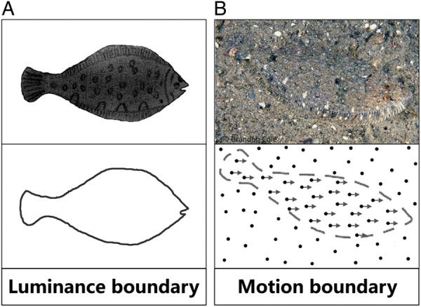
Luminance boundary versus MB. (A) Top: a fish figure on a white background. Bottom: the outline of the fish is defined by the luminance contrast between the fish and its background (luminance boundary). (B) Top: a picture of a sanddab sitting at the bottom of the ocean floor. Because the texture is very similar between the fish and the ocean floor, the fish is remarkably invisible when motionless. Bottom: when the fish moves, the shape of the sanddab (MB) is immediately detectable (also see Supplementary Movie 1).

Where in the visual system are such shape-from-motion cues computed? Traditionally, processing of motion information is associated with the dorsal stream. However, recordings from monkeys have shown that, although area middle temporal cortex (MT/V5) is marked by a high proportion of motion-sensitive neurons, few neurons in MT are responsive to the orientation of MBs (Marcar et al. 1995). Furthermore, MT lesions in monkeys do not eliminate their ability to discriminate shapes defined by motion (Marcar and Cowey 1992; Lauwers et al. 2000). Thus, MT is unlikely to be central to MB processing.

In contrast, evidence points to the role of the ventral pathway in MB detection. Many neurons in areas V4 and inferior temporal cortex (IT) of monkey cortex are selective for the orientation of MBs and demonstrate invariance to boundaries induced by different visual cues (such as luminance, texture, and motion; Sary et al. 1993, 1995; Mysore et al. 2006, 2008). In area V2, an important area upstream from V4, Peterhans and von der Heydt (1993) reported that some neurons in the V2 thick stripes respond well to lines defined by coherent motion, and proposed that these V2 neurons may contribute to the “form-from-motion” detection. This idea was reinforced by the finding that a significant proportion (12%) of V2 neurons exhibit cue-invariant orientation tuning to both luminance- and motion-defined borders (Marcar et al. 2000). However, their responses to motion borders are slower than responses to luminance borders, the authors suggested that the origin of MB detection might be somewhere downstream to area V2. Thus, it is unclear whether V2 plays a critical role in the detection of MB along the ventral stream.

To evaluate the representation of MB in area V2, we ask whether there is any functional organization for MB orientation, and whether such organization is similar to that for luminance-defined orientation. In this study, we used intrinsic signal optical imaging methods in awake, fixating monkeys to map cortical population response of V1 and V2 to MBs. We found robust MB-derived orientation maps in V2, which are much stronger than those in V1. In V2, the orientation maps obtained with MB stimuli and luminance stimuli were similar, demonstrating the presence of cue-invariant orientation maps in V2. Moreover, we found that direction-selective domains in V2 (Lu et al. 2010) were strongly activated by motion contrast in MB stimuli, suggesting that directional neurons in V2 may play an important role in the detection of MB contours.

Materials and Methods

Four adult rhesus monkeys (Macaca mulatta) trained to fixate were used in this optical imaging study. All surgical and experimental procedures conformed to the guidelines of the National Institute of Health and were approved by the institutional Animal Care and Use Committees of Vanderbilt University and Institute of Neuroscience, Chinese Academy of Sciences.

Awake Imaging and Tasks

Monkeys (Cases 1–4) were trained to sit calmly (head fixed) and were required to fixate on a 0.2° fixation spot at the center of the screen during stimulus presentation. Eye position was monitored with an infrared eye tracker (EyeLink 1000, SR Research). Monkeys were rewarded for maintaining fixation within a 2° fixation window. After initial training, a chronic optical imaging chamber was implanted over visual areas V1 and V2 (Chen et al. 2002). One week after recovery from the surgery, we began collection of cortical images in the awake animal. Detailed surgical and imaging procedures are described elsewhere (Roe and Ts'o 1995; Lu et al. 2010; Tanigawa et al. 2010). Optical maps were collected under 632 nm light illumination using the Imager 3001 system (Optical Imaging, Inc., Germantown, NY, USA), the optical signal was collected at a frame rate of 4 Hz (total 16 frames for one trial). The interstimulus interval was 3–4 s. Typically, each experiment contained 8–10 stimulus conditions, which were presented in a random order within a block. Each condition was repeated 70–100 times.

Visual Stimuli

Visual stimuli were created using the ViSaGe system (Cambridge Research Systems Ltd) and presented on a CRT monitor. The stimulus screen was gamma-corrected and positioned 57–140 cm (for different cases) from the eyes. Each stimulus was a 5° (visual angle) square patch that covered the visual field representations of the V1 and V2 regions being imaged. Mean luminance for all stimuli, including the blank stimulus, was kept at 30 cd/m². Random dot patterns (dot size: 0.025–0.08°, 2 pixels; density 3–10%, drift speed: 8 degree/s) were used to obtain direction maps.

MB Stimuli

MB stimuli were created with random dots drifting within a 5° window. The dots were divided into several strips of motion, with dots in neighboring strips drifting in opposite directions; this created the percept of boundaries at the border of the strips. MB stimuli (horizontal and vertical) were illustrated in Supplementary Movie 1. The motion axis of the dots was always at a 45° angle with respect to the strip borders. These borders are invisible when the dots are stationary or when only one frame of the stimulus is presented, but are salient during periods of opposing relative dot motion. The motion borders were stationary during a single trial, but both the spatial offset (phase) and orientation of borders were randomized from trial to trial. The width of the strips was either 0.4 or 0.8° of visual angle; this is equivalent to a spatial frequency (SF) of 1.25 or 0.625 cycles/degree (close to the peak SF selectivity of V1 and V2, Lu and Roe 2007). Since the results were similar for both SF (not shown), the imaging data of the 2 SF were averaged. Single dots were 0.025–0.08° in diameter (depending on the screen distance) and covered a total of 10% of the screen area. Dots drifted at a speed of 1–2 degree/s in order to minimize the potential confound caused by motion streak effect (Geisler 1999; Rasch et al. 2013). In a single imaging session, the orientations of MB were one of the following pairs (0 and 90°, or 45 and 135°) and were presented in a randomly interleaved fashion.

Temporal Boundary Stimuli

As a control for dynamic cues and motion streak discontinuities at the virtual borders in the MB stimuli (Sary et al. 1993), temporal boundary (TB) stimuli were created in a similar way as MB stimuli. The only difference between TB and MB stimuli is that, in TB stimuli, all dots were moving in the same direction and speed and therefore lacked motion contrast information. The dots of the TB stimuli also appeared and disappeared at the virtual boundaries, and contained the same motion streak discontinuities as MB stimuli. Perceptually, TB stimuli evoke a weaker orientation sensation than MB stimuli. Other parameters, including dot size, density, and boundary periodicity, were the same between TB and MB. Supplementary Movie 2 illustrated the horizontal- and vertical-oriented TB stimuli.

Data Analysis

Support Vector Machine Maps

In this study, we used support vector machine (SVM) maps instead of conventional subtraction maps. It has been shown that SVM maps typically have a higher signal–noise ratio than conventional subtraction maps (Xiao et al. 2008, also see Supplementary Fig. 1). SVM is a pattern classification algorithm commonly used for extracting stimulus preference from functional imaging data (Kamitani and Tong 2005; Xiao et al. 2008). Similar to subtraction maps, an SVM map reveals differential information between 2 sets of images. In an SVM map, each pixel's gray value represents the relative contribution that pixel makes to the classification. The Matlab SVM program was provided by Chang and Lin (LIBSVM: a library for support vector machines, 2001; available at http://www.csie.ntu.edu.tw/~cjlin/libsvm/). For each stimulus condition, a percentage change map (dR/R) was first calculated using the following formula: dR/R = (R_i − R₀)/R₀, in which R_i are single frames between frames 11 and 16, R₀ is the average of frame 1–2. The resulting images were then used for SVM classification (similar to Xiao et al. 2008). One SVM weight map was obtained for 2 sets of images corresponding to the comparison conditions. Unless otherwise specified, all SVM maps were clipped at 2.5 SD on each side of the map median for display.

Orientation Domain Location Comparison

To compare the locations of orientation domains obtained with luminance gratings (LGs) and MB stimuli, we used a thresholding method to identify domain locations. LG orientation maps were smoothed (low-pass circular mean filter, 0.25 mm). The top 10% of most responsive horizontal and vertical pixels were selected, respectively (Ramsden et al. 2001). Artifacts due to blood vessel noise were removed based on blood vessel maps.

Correlation Coefficient

For comparing the similarity between 2 orientation maps, 2D correlation coefficient was calculated; this correlation value were converted to Fisher's z′ score for linear comparison. The spatial specificity of each correlation score was verified by estimate the P-value of the raw z′ score with its bootstrap sample z′ score distribution. A bootstrap sample was carried out with shuffled pixels of one orientation map, used then to calculate the correlation coefficient with another orientation map, and repeated 1000 times (Maus et al. 2013).

Response Profile

Population response profiles were calculated to assess the overall orientation response in a particular map. This method was first introduced by Basole et al. (2003). Briefly, the orientation angle map obtained from vector analysis (Bosking et al. 1997) was used as the reference angle map. For a specific subtraction map under examination, the top 40% pixels in magnitude map from vector analysis were categorized into 20 orientation-selective groups (0–180°) according to their orientation angles in the reference angle map. Pixel values within each group were then summed. The resulting response profile reflects whether a specific orientation-preferring group of pixels were activated in the map. If a map has no spatial correlation to the corresponding orientation map (the reference angle map), the profile will be flat.

Frame Misalignment Correction

In awake imaging, motion noise is often induced due to animal movement, irregular respiration, body position, etc. The maximum shift is about 50–100 µm (3–6 pixels). We calculated the movement offline and realigned the images frame-by-frame. Detailed alignment method is discussed elsewhere (Chen et al. 2002; Roe 2007).

Results

Monkeys were imaged while performing on a 3.5-s visual fixation task. Intrinsic optical signals were acquired from V1 and V2 (Fig. 2A). Figure 2B–I shows maps obtained from Case 1. Surface blood vessel map (Fig. 2B) was collected for day-to-day image alignment. An SVM method was used for calculating difference maps (Xiao et al. 2008, also see Materials and Methods and Supplementary Fig. 1). Pixel values in a SVM difference map represent the pixels' relative contribution to separating cortical responses to 2 sets of stimulus conditions. Typical functional maps (e.g., ocular dominance maps; Fig. 2C) were also collected during the chamber implant session when monkeys were anesthetized.

Figure 2.

V2 has robust MB orientation maps. (A) Illustration of cortical areas (V1 and V2) of a macaque monkey where intrinsic optical signals were imaged. (B) Surface blood vessel map of the imaged region in Case 1. Images are all from this region. (C) Ocular dominance map shows columns of eye-dominance regions in V1, but not in V2. Dotted line: the border between areas V1 and V2. (D and E) Two horizontal versus vertical MB orientation maps for MBs induced by random dots moving along 45° axis (D) or 135° axis (E). The response in V2 is much stronger than that in V1. These 2 maps are very similar, indicating that MB orientation responses do not depend on the moving directions of the random dots. (F) Horizontal versus vertical orientation map obtained with LGs. Three maps in D–F exhibit similar orientation-preference patterns in V2. (G–I) Another set of orientation maps similar to D–F. These 45° versus 135° orientation maps were obtained with MBs induced by 0° moving dots (G), 90° moving dots (H), or with LGs (I). All 3 maps exhibit highly similar orientation-preference patterns in V2, but not in V1. All maps were clipped at the same level (median ± 2.5 SD) for display. About 1 mm scale bar applies to all maps. A: anterior; M: medial.

Presence of Orientation Maps for MB in V2

MB stimuli were created with strips of random dots drifting in opposite directions (see Materials and Methods). In a pair of comparison conditions (e.g., 2 stimuli illustrated in Fig. 2D, also see Supplementary Movie 1), dot motion was the same (45°); the only difference was the orientation of the MB. As a result, the differential method removes the common components of the 2 stimuli (the dot motion), and leaves the MB orientation differences which produced a strong orientation map in V2 and a much weaker response in V1 (Fig. 2D).

To further test whether this response was due to the MB component of the stimuli, we devised another stimulus with the same MBs, but induced by different random dot motion (135°). If the V2 map truly represents the orientation information of the MB, the MB orientation map should be independent of the axis of dot motion. As shown in Figure 2E, very similar activation patterns were obtained with dots moving at either 45° or 135° (compare Fig. 2D and E). The 2D correlation coefficient between the 2 V2 activation patterns was 0.80. The fact that very similar maps were obtained despite the different motion content indicates that these V2 activation patterns were not due to the axis of the dot motion but rather evoked by the orientation of the MB.

We observed that the behavior of V1 was quite different from that of V2. While V1 also exhibited some evident responsiveness to MB (lower part of the maps in Fig. 2D,E), the strength of the pattern was much weaker than that in V2. The 2D correlation coefficient between the V1 activation in these 2 maps was only 0.19, likely due to the lower signal/noise ratio in V1. V1 thus exhibits a much weaker ability to detect MB orientation. The borders between the strong and weak orientation activation regions in Figure 2D,E were also congruent with that defined by the ocular dominance map (Fig. 2C). For LGs, comparison of 2 orthogonal orientation conditions revealed clear orientation maps in both V1 and V2 (Fig. 2F). Unlike the different V1/V2 responses in MB orientation maps, orientation domains in V1 and V2 of the LG maps had comparable response strengths.

Similar results were obtained for MBs presented at different orientations. For MB orientation maps derived from 45° versus 135° orientation (induced with horizontal, Fig. 2G, and vertical, Fig. 2H moving dots), similar response trends were observed. Both maps had similar MB orientation response patterns in V2 (r′ = 0.78), compared with weakly correlated orientation patterns in V1 (r′ = 0.09). Thus, correlation analysis support that there are orientation maps for MB in area V2. This finding was consistent across all 4 monkeys (4 chambers) we imaged (Supplementary Fig. 2). Furthermore, for each case, repeated imaging on different days also revealed the same orientation maps, indicating that these MB orientation response maps are stable and not artifactual.

Colocalized V2 Orientation Maps for MB and LG Stimuli

The MB orientation domains appeared to match the LG orientation domains in V2 (compare Fig. 2D, E, and F; Fig. 2G, H, and I). To measure this similarity, we first examined the spatial correspondence of 2 sets of V2 orientation domains in MB and LG orientation maps. As shown in Figure 3A, we obtained orientation domain outlines by selecting the most responsive pixels (top 10% pixels for horizontal and vertical orientations, respectively) from the LG orientation map (Fig. 3A left panel, brown outlines: horizontal domains; cyan outlines: vertical domains). These outlines were then overlaid on the MB orientation map (Fig. 3A, right panel). By comparing the outlines and MB orientation responses, it is evident that these 2 sets of orientation domains were closely matched with respect to their locations, shapes, and activation signs (black or white).

Figure 3.

V2 has higher MB orientation selectivity than V1. (A) Horizontal versus vertical orientation maps for LG (left panel) and MB (right panel) stimuli overlaid with the same orientation domain outlines (yellow: horizontal domains; cyan: vertical domains). The orientation outlines were obtained from LG orientation map. Two maps have very similar orientation response patterns in V2. (B) Fisher's z′ score for pixel-based correlations between LG and MB orientation maps in V1 and V2. LG and MB orientation maps have higher similarity in V2 than those in V1 (paired two-tailed t-test, P = 0.017, n = 4). V1 and V2 correlation values are both significantly higher than those obtained from bootstraped pairs (P < 0.001, see Materials and Methods). (C) Orientation response profiles for LG (solid curves) and MB (dotted curves) from Case 1. Red curves are obtained from V2, and black curves are from V1. X axis denotes the measured orientation of the orientation maps, centered at the stimulus orientation. See Supplementary Figure 2 for all other cases. (D) Peak orientations obtained from response profiles (n = 4) are not different from stimulus orientations (V1: P = 0.76; V2: P = 0.09). (E) Averaged V1 and V2 response amplitudes obtained from peaks of response profiles (n = 4). Compared with V1, V2 shows a larger response for both LG (P = 0.03) and MB (P = 0.008) stimuli. (F) V2/V1 response ratios, calculated based on values in E, are higher for MB than for LG (P = 0.03). (G) MB/LG response ratios, also calculated based on values in E, are higher for V2 than for V1 (P = 0.022). Error bars in B–F: SEM. Scale bar = 1 mm.

For V1, weak orientation domains were also observed in MB orientation maps. In Figure 3A, MB orientation responses in V1 also had a tendency to colocalize with V1 orientation domains: some darker pixels tended to colocalize with brown outlines (horizontal domains), while some brighter pixels tended to colocalize with cyan outlines (vertical domains). We did pixel-wise correlation for all V1 pixels between the 2 maps. For linear comparison, correlation coefficient was transformed to Fisher z′ value. The correlation score also showed significant correlation between V1 response patterns in LG and MB orientation maps (Fig. 3B, black dots, r′ = 0.3629, z′ = 0.3802, P < 0.001; see Materials and Methods). However, this value was much lower than that for V2 (Fig. 3B, red dots, r′ = 0.7695, z′ = 1.0191, P < 0.001). The significant higher (P = 0.017, paired t-test, n = 4) correlation scores in V2 indicate a systematic difference between these 2 areas (Fig. 3B).

Compare with V1: Increased MB Orientation Response in V2

In all 4 cases, MB and LG stimuli activated similar orientation maps in V2 (Fig. 3A and Supplementary Fig. 2). To quantitatively compare the response magnitudes to MB and LG, we calculated response profiles for different visual areas (V1 and V2) and different stimuli (MB and LG), based on MB and LG orientation maps. Response profile is a measurement used to quantitatively identify which orientation domains are preferentially activated in a difference map (Basole et al. 2003). A flat profile means that all orientation domains are equally activated (showing no orientation preference). Figure 3C shows the response profiles from Case 1, the X axis denotes the measured orientation of the orientation maps, centered at the stimulus orientation. Similar to V1 and V2 responses to LG stimuli (solid curves), V1 and V2 responses to MB stimuli (dotted curves) also showed a unimodal distribution peaked at the stimulus orientation. This indicates that the V1 and V2 patterns in the MB orientation map truly represent the MB orientation in the stimuli. We found that this is true for all 4 cases, all MB response profiles peaked around the stimulus orientation, and no significant differences were found for peak orientations between MB and LG conditions (Fig. 3D, paired t-test, V1: P = 0.76; V2: P = 0.09). All these indicate that similar orientation-preferring pixels were activated by MB and LG stimuli.

Compared with V2, V1 showed a lower orientation response to both LG and MB stimuli. We further evaluated peak magnitudes of the response profiles to investigate whether the lower V1 responses to MB are attributable to its generally lower responses to oriented stimuli. Figure 3E plots the average peak amplitudes of response profiles for LG and MB stimuli (n = 4). The average V1 response to MB of 0.08 ± 0.007 was significantly lower than the V2 MB response (0.24 ± 0.03, P = 0.008, paired t-test, n = 4). Similarly, the decrease in the V1 from the V2 response to LG was also significant (V1: 0.65 ± 0.11; V2: 1.00, P = 0.03). The V2/V1 response ratios for LG and MB stimuli are shown in Figure 3F. For MB, the V2/V1 ratio was 3.0, higher than that for LG stimuli (V2/V1 = 1.6; P = 0.03). This suggests that the stronger V2 responses to MB cannot be explained by a simple increase in gain of V1 orientation responses. Similarly, the MB/LG response ratio was significant larger (P = 0.02) in V2 (0.24) than that in V1 (0.12), confirm that a significant increase similarity of MB and LG orientation responses in V2 (Fig. 3G).

MB Responses Relies on the Motion Contrast Information

Besides the motion direction contrast component in the MB stimulus, moving dots are appearing/disappearing at the border. This creates both temporal dynamic cues and motion streak discontinuities at the borders (illustrated in Supplementary Fig. 3), which may possibly contribute to the MB responses we observed. To investigate whether the latter 2 components could lead to a differential response in the orientation maps, we constructed control stimuli which we term TB stimuli (Supplementary Movie 2). Similar to the MB stimulus, the TB stimulus contains strips of moving dots. Moving dots in TB stimulus also appear/disappear at the virtual boundaries and have the same duration, size, and luminance as those in MB stimulus. The only difference is that, in a TB stimulus, all dots are moving in the same direction and thus lack motion direction contrast. Perceptually, it is much more difficult to detect borders in TB than in MB stimuli. Figure 4 shows the orientation responses to TB, MB, and LG stimuli in 2 cases (Cases 2 and 3). In both cases, the TB stimulus only elicits a very weak orientation response in either V1 or V2 (Fig. 4A,D). This contrasted sharply with MB-activated orientation domains in V2 (Fig. 4B,E) and with LG-activated orientation domains in both V1 and V2 (Fig. 4C,F). The different results from TB and MB indicate that it is not the temporal dynamic cues or the motion streak discontinuities, but the motion contrast component (direction differences in MB), that is crucial for generating strong MB orientation responses in V2. In the present study, we used a relatively slow dot moving speed in our MB and TB stimuli (1–2 degree/s), which minimized the motion streak effects (Rasch et al. 2013). When dot speed increases, it is reasonable to predict that the other 2 components will contribute more to the orientation map.

Figure 4.

MB response relies on the motion contrast information. All maps are orientation maps obtained from different stimuli (columns) or different cases (rows). (A–C) Comparison of orientation maps for 3 different stimuli in Case 2: TB (A), MB (B), and LG (C). In TB stimulus, all dots were moving at the same direction so it lacks motion contrast information. The TB stimulus is otherwise the same as the MB stimulus (including dot appear/disappear at the virtual borders). Unlike orientation maps for MB (B) and LG (C), no obvious orientation pattern is observed in the TB orientation map (A). (D–F) Similar to (A–C), orientation maps from Case 3. Weak orientation activity was observed in V2 for the TB stimulus (D). Scale bar = 1 mm. A: anterior; M: medial; L: lateral.

The Neural Correlates of Motion Contrast Representation: A Proposed Model

How is motion contrast information computed and used for MB orientation coding? While there are motion-sensitive neurons in many areas (V1, V2, MT etc.), we propose that direction-selective neurons in V2 are likely to play an important role in this analysis. We have previously shown that V2 direction neurons cluster and form direction domains in thick and pale stripes (Lu et al. 2010), which suggests that they are actively processing motion information in this area. We further hypothesize that V2 direction neurons contribute (either directly or indirectly) to the computation of motion contrast, which is essential for MB response. We predict a colocalization of motion contrast responses and direction domains in V2.

We first calculated direction maps in V2, by contrasting opposite moving dot conditions. As shown in Figure 5A, strong direction domains were present in V2. These domains covered a smaller part of the full V2 orientation map, consistent with our previous report (Lu et al. 2010). We then calculated motion axis maps for MB and TB stimuli (Fig. 5B,C). Motion axis maps are calculated by pooling all conditions with the same dot motion axis and contrasting 2 such groups that have orthogonal motion axes (see stimulus illustrations under Fig. 5B,C). For simplicity, only half of the stimulus conditions on each side of the comparisons are shown. The other half are stimuli having orthogonal MB/TB. The motion axis maps for MB stimulus (Fig. 5B, red arrowheads) showed regions of preference to motion axis that were remarkably similar in location to the direction domains in V2 (Fig. 5A, red arrowheads). But the TB stimulus motion axis map was basically flat (Fig. 5C). The differential activation in the MB and TB axis maps is likely due to the differences in their stimuli (i.e., the presence or absence of motion contrast). These results suggest that neurons in V2 direction domains may contribute to the detection of motion contrast, which is essential for the MB detection.

Figure 5.

Colocalization of motion contrast response and direction domains in V2. (A) Motion direction preference map (obtained by comparing random dot conditions moving in opposite directions). Red arrowheads indicate V2 direction domains. (B and C) Axis-of-motion maps obtained by comparing stimulus conditions in which random dots moving along 2 orthogonal axes (see stimulus illustrations below the maps). Axis map for MB (B) clearly shows an activation pattern in V2 (red arrowheads), whereas axis map for TB (C) shows weak (if any) patterns, presumably due to the motion contrast information in the MB stimuli. The direction-preferring domains (A) in V2 spatially match the location of the regions sensitive to motion contrast (B). This suggests that direction-preferring neurons may be preferentially involved in detecting motion contrast. Scale bar = 1 mm. A: anterior; L: lateral.

Figure 6 shows this hypothesis. Direction neurons in V2 direction domains compute motion information (Fig. 6A). These directional signals are then used to compute motion contrast in neurons in the same domains (Fig. 6B). Aligned motion contrast signals are finally integrated by orientation-selective neurons in V2 thick and pale stripes to generate MB orientation detection (Fig. 6C). Each of these 3 steps has supporting evidence including V2 direction maps for motion responses in V2 (Lu et al. 2010 and this study); V2 MB axis maps for motion contrast responses in V2 (this study); and V2 MB orientation maps for MB orientation responses (this study). For simplicity, we did not include potential feedforward contribution from V1 (e.g., direction neurons in V1) or feedback influence from higher-level areas (e.g., MB selectivity in V4). We do not exclude the possibility of their contributions.

Figure 6.

A proposed model for MB detection in V2. Motion information is first detected by direction-selective neurons in V1 and V2 (A). Local motion contrast information is then detected in V2 direction domains (B). Such activation is crucial for generating of MB orientation response which is coded in orientation-selective neurons in V2 orientation domains (C). Supporting evidence include direction map in V2, motion contrast response in direction domains, and MB orientation maps.

Discussion

In this study, we quantitatively measured the population response of V1 and V2 to MB stimuli. We found significant orientation-preferring responses to MB in area V2. Such responses form an orientation map that colocalizes with the known V2 orientation map, indicating invariance of orientation response across quite different stimuli. In contrast, orientation response to MB in V1 is much weaker. Furthermore, such MB response in V2 is tightly related to the activity of V2 direction domains, which are likely sensitive to the motion contrast information in the MB stimulus. Unlike previous optical imaging studies in anesthetized animals (e.g., Ramsden et al. 2001; Pan et al. 2012), this study imaged a response in awake monkeys which is closer to normal perceptual states. We also adopted SVM pattern classification methods into imaging data analysis, which improved the signal–noise ratio and provided better measurement of our data.

MB Response in V2

The results of the present study extend previous electrophysiological findings that some V2 neurons can represent orientations defined by moving dots. In anesthetized monkeys, Marcar et al. (2000) found that about 12% of V2 neurons displayed the same orientation selectivity to both MB and luminance boundaries. Our data further demonstrate that such response to MB also forms a functional map that colocalizes with the orientation map in V2 derived by LGs. We also find dramatically weaker responses to MB in V1 than in V2. The new results add strong support to the view that higher-order cue-invariant orientation representation arises prominently at the level of V2.

Marcar et al. (2000) found that kinetic boundary-selective neurons respond 40-ms slower than kinetic boundary non-selective neurons, and hypothesized that such selectivity may be computed in downstream areas (e.g., V3 and V4). A later study from the same group (Mysore et al. 2006) showed that area V4 contains neurons (10–20%) selective for MB orientation. The imaging method used in our study does not allow us to measure the temporal difference between MB and LG response. The hemodynamic responses we obtained also contain contributions from both spike activity and membrane potentials (Zepeda et al. 2004). Thus, we are unable to exclude the possibility of feedback contribution. However, we provide evidence showing that, in addition to this possible feedback contribution, MB response in V2 could be computed locally within V2 (see Discussion below). Such local computation may cause longer delays for MB responses and account for the 40-ms latency difference. These 2 processes (local and feedback) are not necessarily mutually exclusive, and can coexist in V2.

We further suggest that V2 direction neurons are crucial for the MB detection process. First, motion signal is abundant in V2. It has been shown that V2 contains a large number of direction-selective neurons (∼15%) located in thick stripes (Hubel and Livingstone 1987; von der Heydt and Peterhans 1989; Levitt et al. 1994). Considering the large size of area V2, the number of direction neurons in V2 may be comparable to that in area MT. Secondly, the presence of direction maps in V2 (Lu et al. 2010) further suggests that motion processing is a fundamental and important feature of V2. Thirdly, as we showed in this study, neurons in V2 direction domains exhibit stronger activation when a stimulus contains motion contrast information (Fig. 5B). All the evidence suggests that the direction neurons in V2 provide the motion information for the “form-from-motion” detection originally described by Peterhans and von der Heydt (1993). Currently, it is unclear how motion contrast information is transformed to orientation information. V2 direction domains cover smaller areas than orientation domains (compare Figs 4C and 5A, also see Lu et al. 2010). So, it is unlikely that only V2 direction neurons code MB orientation. In our model (Fig. 6), we propose that orientation neurons receive input from “motion contrast” neurons to generate MB orientation selectivity. These “motion contrast” neurons are located in the V2 direction domains. They could be direction neurons or neurons receiving mixed inputs from direction neurons.

Previous studies have shown that V2 neurons are capable of detecting boundaries induced with different types of cues, such as illusory contours formed with abutting lines (Peterhans and von der Heydt 1989; von der Heydt and Peterhans 1989; Ramsden et al. 2001) or disparity edges based on different binocular disparity cues (von der Heydt et al. 2000; Bredfeldt and Cumming 2006). V2 neurons also have a better representation of natural texture than V1 neurons do, suggesting that V2 is significantly different from V1 in analyzing spatial features (Freeman et al. 2013). Our results, together with previous single-unit findings (Marcar et al. 2000), add motion cues to contour detection in V2. Area V2 thus seems to have the capability of general contour detection and provides a platform for contour integration. If this is true, then it is possible that V4 may largely inherit the cue-invariant boundary detection from V2. Under natural scene contexts (e.g., global shape recognition), it is likely that MB response in V2 is further strengthened by top-down feedback from higher-level areas (e.g., V4). However, feedback is unlikely to be the sole means of generating MB response in V2, as monkeys with lesions of V4 are still capable of distinguishing orientations of higher-order contours (De Weerd et al. 1996). In contrast, monkeys with lesions of V2 are unable to do so (Merigan et al. 1993). Thus, together with other studies, our data strongly suggest that V2 is a level essential for higher-order contour perception.

MB Response in V1

In maps we obtained with MB stimuli, V1 only show very weak orientation maps. Although the pooled response (in response profile) reveals a statistically significant MB response, it is clearly different from the robust maps observed in V2. Such differences are consistent with single-cell studies, where a small percentage (3.8%) of sampled V1 neurons demonstrates weak selectivity to MB, in comparison with a larger proportion (12%) in V2 that exhibited strong selectivity for MB (Marcar et al. 2000). Due to their small receptive field (RF) size, V1 neurons are likely incapable of extracting orientation information from MB. The weakness of MB response also suggests that V1 is not the defining stage. Feedback projections from orientation domains in V2 target a broad range of orientation domains in V1 (Shmuel et al. 2005). Thus, it is possible that such weakly orientation biased feedback influence from V2 is detected at the population level in our imaging results.

Although V1 does not appear to code MB orientation, it may still play a role in detecting local motion contrast in the MB stimulus. In comparison with homogenous motion stimuli, V1 neurons are better activated by motion difference (either direction or speed) between their RF center and surround, commonly known as the surround-inhibition effect (Shen et al. 2007). Such a property may result in generation of a retinotopic map of local motion contrasts (along the motion border). Experimentally, a V1 retinotopic representation of MB has been demonstrated in macaque monkeys (Lamme 1995) and also in humans (Reppas et al. 1997). Such a map is believed to be strengthened by top-down signals without local explicit information of border orientation. Such a map may also be used by downstream areas (e.g., V2) to extract orientation information explicitly.

Overall, our findings demonstrate a systematic orientation information extraction in V2. As demonstrated by the cue-invariant maps in this study, V2 is likely a stage at which contours recognition is generalized. This contour recognition process is an important stage, which contributes to further shape integration processes in areas such as V4 and IT.

Supplementary Material

Supplementary material can be found at: http://www.cercor.oxfordjournals.org/.

Funding

This work was supported by grants from the National Natural Science Foundation of China (31371111 to H.D.L.); the Hundred Talent Program of the Chinese Academy of Sciences (H.D.L.), NIH EY 11744 (A.W.R.), and Vanderbilt Vision Core Grant.

References

- Basole A, White LE, Fitzpatrick D. 2003. Mapping multiple features in the population response of visual cortex. Nature. 423:986–990. [DOI] [PubMed] [Google Scholar]
- Bosking WH, Zhang Y, Schofield B, Fitzpatrick D. 1997. Orientation selectivity and the arrangement of horizontal connections in tree shrew striate cortex. J Neurosci. 17:2112–2127. [DOI] [PMC free article] [PubMed] [Google Scholar]
- Bredfeldt CE, Cumming BG. 2006. A simple account of cyclopean edge responses in macaque V2. J Neurosci. 26:7581–7596. [DOI] [PMC free article] [PubMed] [Google Scholar]
- Chen LM, Heider B, Williams GV, Healy FL, Ramsden BM, Roe AW. 2002. A chamber and artificial dura method for long-term optical imaging in the monkey. J Neurosci Methods. 113:41–49. [DOI] [PubMed] [Google Scholar]
- De Weerd P, Desimone R, Ungerleider LG. 1996. Cue-dependent deficits in grating orientation discrimination after V4 lesions in macaques. Visual Neurosci. 13:529–538. [DOI] [PubMed] [Google Scholar]
- Freeman J, Ziemba CM, Heeger DJ, Simoncelli EP, Movshon JA. 2013. A functional and perceptual signature of the second visual area in primates. Nat Neurosci. 16:974–981. [DOI] [PMC free article] [PubMed] [Google Scholar]
- Geisler WS. 1999. Motion streaks provide a spatial code for motion direction. Nature. 400:65–69. [DOI] [PubMed] [Google Scholar]
- Hubel DH, Livingstone MS. 1987. Segregation of form, color, and stereopsis in primate area 18. J Neurosci. 7:3378–3415. [DOI] [PMC free article] [PubMed] [Google Scholar]
- Kamitani Y, Tong F. 2005. Decoding the visual and subjective contents of the human brain. Nat Neurosci. 8:679–685. [DOI] [PMC free article] [PubMed] [Google Scholar]
- Lamme VAf. 1995. The neurophysiology of figure-ground segregation in primary visual cortex. J Neurosci. 15:1605–1615. [DOI] [PMC free article] [PubMed] [Google Scholar]
- Lauwers K, Saunders R, Vogels R, Vandenbussche E, Orban GA. 2000. Impairment in motion discrimination tasks is unrelated to amount of damage to superior temporal sulcus motion areas. J Comp Neurol. 420:539–557. [DOI] [PubMed] [Google Scholar]
- Levitt JB, Kiper DC, Movshon JA. 1994. Receptive fields and functional architecture of macaque V2. J Neurophysiol. 71:2517–2542. [DOI] [PubMed] [Google Scholar]
- Lu HD, Chen G, Tanigawa H, Roe AW. 2010. A motion direction map in macaque V2. Neuron. 68:1002–1013. [DOI] [PMC free article] [PubMed] [Google Scholar]
- Lu HD, Roe AW. 2007. Optical imaging of contrast response in macaque monkey V1 and V2. Cereb Cortex. 17:2675–2695. [DOI] [PubMed] [Google Scholar]
- Marcar VL, Cowey A. 1992. The effect of removing superior temporal cortical motion areas in the macaque monkey: II. Motion discrimination using random dot displays. Eur J Neurosci. 4:1228–1238. [DOI] [PubMed] [Google Scholar]
- Marcar VL, Raiguel SE, Xiao D, Orban GA. 2000. Processing of kinetically defined boundaries in areas V1 and V2 of the macaque monkey. J Neurophysiol. 84:2786–2798. [DOI] [PubMed] [Google Scholar]
- Marcar VL, Xiao DK, Raiguel SE, Maes H, Orban GA. 1995. Processing of kinetically defined boundaries in the cortical motion area MT of the macaque monkey. J Neurophysiol. 74:1258–1270. [DOI] [PubMed] [Google Scholar]
- Maus G, Fischer J, Whitney D. 2013. Motion-dependent representation of space in area MT+. Neuron. 78:554–562. [DOI] [PMC free article] [PubMed] [Google Scholar]
- Merigan WH, Nealey TA, Maunsell JH. 1993. Visual effects of lesions of cortical area V2 in macaques. J Neurosci. 13:3180–3191. [DOI] [PMC free article] [PubMed] [Google Scholar]
- Mysore SG, Vogels R, Raiguel SE, Orban GA. 2006. Processing of kinetic boundaries in macaque V4. J Neurophysiol. 95:1864–1880. [DOI] [PubMed] [Google Scholar]
- Mysore SG, Vogels R, Raiguel SE, Orban GA. 2008. Shape selectivity for camouflage-breaking dynamic stimuli in dorsal V4 neurons. Cereb Cortex. 18:1429–1443. [DOI] [PubMed] [Google Scholar]
- Pan Y, Chen M, Yin J, An X, Zhang X, Lu Y, Gong H, Li W, Wang W. 2012. Equivalent representation of real and illusory contours in macaque V4. J Neurosci. 32:6760–6770. [DOI] [PMC free article] [PubMed] [Google Scholar]
- Peterhans E, von der Heydt R. 1993. Functional organization of area V2 in the alert macaque. Eur J Neurosci. 5:509–524. [DOI] [PubMed] [Google Scholar]
- Peterhans E, von der Heydt R. 1989. Mechanisms of contour perception in monkey visual cortex. II. Contours bridging gaps. J Neurosci. 9:1749–1763. [DOI] [PMC free article] [PubMed] [Google Scholar]
- Ramsden BM, Hung CP, Roe AW. 2001. Real and illusory contour processing in area V1 of the primate: a cortical balancing act. Cereb Cortex. 11:648–665. [DOI] [PubMed] [Google Scholar]
- Rasch MJ, Chen M, Wu S, Lu HD, Roe AW. 2013. Quantitative inference of population response properties across eccentricity from motion-induced maps in macaque V1. J Neurophysiol. 109:1233–1249. [DOI] [PMC free article] [PubMed] [Google Scholar]
- Regan D. 1986. Form from motion parallax and form from luminance contrast: vernier discrimination. Spat Vis. 1:305–318. [DOI] [PubMed] [Google Scholar]
- Regan D. 1989. Orientation discrimination for objects defined by relative motion and objects defined by luminance contrast. Vis Res. 29:1389–1400. [DOI] [PubMed] [Google Scholar]
- Reppas JB, Niyogi S, Dale AM, Sereno MI, Tootell RBH. 1997. Representation of motion boundaries in retinotopic human visual cortical areas. Nature. 388:175–179. [DOI] [PubMed] [Google Scholar]
- Roe AW. 2007. Long-term optical imaging of intrinsic signals in anesthetized and awake monkeys. Appl Opt. 46:1872–1880. [DOI] [PubMed] [Google Scholar]
- Roe AW, Ts'o DY. 1995. Visual topography in primate V2: multiple representation across functional stripes. J Neurosci. 15:3689–3715. [DOI] [PMC free article] [PubMed] [Google Scholar]
- Sary G, Vogels R, Kovacs G, Orban GA. 1995. Responses of monkey inferior temporal neurons to luminance-, motion-, and texture-defined gratings. J Neurophysiol. 73:1341–1354. [DOI] [PubMed] [Google Scholar]
- Sary G, Vogels R, Orban GA. 1993. Cue-invariant shape selectivity of macaque inferior temporal neurons. Science. 260:995–997. [DOI] [PubMed] [Google Scholar]
- Shen Z-M, Xu W-F, Li C-Y. 2007. Cue-invariant detection of centre–surround discontinuity by V1 neurons in awake macaque monkey. J Physiol. 583:581–592. [DOI] [PMC free article] [PubMed] [Google Scholar]
- Shmuel A, Korman M, Sterkin A, Harel M, Ullman S, Malach R, Grinvald A. 2005. Retinotopic axis specificity and selective clustering of feedback projections from V2 to V1 in the owl monkey. J Neurosci. 25:2117–2131. [DOI] [PMC free article] [PubMed] [Google Scholar]
- Tanigawa H, Lu HD, Roe AW. 2010. Functional organization for color and orientation in macaque V4. Nat Neurosci. 13:1542–1548. [DOI] [PMC free article] [PubMed] [Google Scholar]
- von der Heydt R, Peterhans E. 1989. Mechanisms of contour perception in monkey visual cortex. I. Lines of pattern discontinuity. J Neurosci. 9:1731–1748. [DOI] [PMC free article] [PubMed] [Google Scholar]
- von der Heydt R, Zhou H, Friedman HS. 2000. Representation of stereoscopic edges in monkey visual cortex. Vis Res. 40:1955–1967. [DOI] [PubMed] [Google Scholar]
- Xiao Y, Rao R, Cecchi G, Kaplan E. 2008. Improved mapping of information distribution across the cortical surface with the support vector machine. Neural Netw. 21:341–348. [DOI] [PMC free article] [PubMed] [Google Scholar]
- Zepeda A, Arias C, Sengpiel F. 2004. Optical imaging of intrinsic signals: recent developments in the methodology and its applications. J Neurosci Methods. 136:1–21. [DOI] [PubMed] [Google Scholar]
Associated Data
This section collects any data citations, data availability statements, or supplementary materials included in this article.