Basic Reproduction Number and Transmission Dynamics of Common Serogroups of Enterohemorrhagic Escherichia coli

ABSTRACT

Understanding the transmission dynamics of pathogens is essential to determine the epidemiology, ecology, and ways of controlling enterohemorrhagic Escherichia coli (EHEC) in animals and their environments. Our objective was to estimate the epidemiological fitness of common EHEC strains in cattle populations. For that purpose, we developed a Markov chain model to characterize the dynamics of 7 serogroups of enterohemorrhagic Escherichia coli (O26, O45, O103, O111, O121, O145, and O157) in cattle production environments based on a set of cross-sectional data on infection prevalence in 2 years in two U.S. states. The basic reproduction number (R₀) was estimated using a Bayesian framework for each serogroup based on two criteria (using serogroup alone [the O-group data] and using O serogroup, Shiga toxin gene[s], and intimin [eae] gene together [the EHEC data]). In addition, correlations between external covariates (e.g., location, ambient temperature, dietary, and probiotic usage) and prevalence/R₀ were quantified. R₀ estimates varied substantially among different EHEC serogroups, with EHEC O157 having an R₀ of >1 (∼1.5) and all six other EHEC serogroups having an R₀ of less than 1. Using the O-group data substantially increased R₀ estimates for the O26, O45, and O103 serogroups (R₀ > 1) but not for the others. Different covariates had distinct influences on different serogroups: the coefficients for each covariate were different among serogroups. Our modeling and analysis of this system can be readily expanded to other pathogen systems in order to estimate the pathogen and external factors that influence spread of infectious agents.

IMPORTANCE In this paper we describe a Bayesian modeling framework to estimate basic reproduction numbers of multiple serotypes of Shiga toxin-producing Escherichia coli according to a cross-sectional study. We then coupled a compartmental model to reconstruct the infection dynamics of these serotypes and quantify their risk in the population. We incorporated different sensitivity levels of detecting different serotypes and evaluated their potential influence on the estimation of basic reproduction numbers.

INTRODUCTION

Shiga toxin-producing Escherichia coli (STEC) can cause diarrhea, hemorrhagic colitis, and hemolytic-uremic syndrome, which is a major cause of acute renal failure in children (1). STEC O157:H7 is the most common serogroup linked to human cases and has received the most attention from public health and research perspectives (2), including designation as an adulterant in some food products. In recent years, STEC serogroups that express an O surface antigen other than O157, known collectively as non-O157, have also emerged as important pathogens. Enterohemorrhagic E. coli (EHEC) strains are a subset of STEC characterized by the expression of an O surface antigen and the presence of Shiga toxin and intimin genes. Non-O157 serogroups are estimated to cause 64% of domestically acquired STEC infections in the United States (2). Six non-O157 STEC serogroups have recently been designated adulterants of nonintact beef products and ground meat: O26, O45, O103, O111, O121, and O145. The most common source of exposure and subsequent infection in humans is food (3–5). Undercooked contaminated beef, unpasteurized milk, produce, and unpasteurized juices, among other contaminated foods, have been associated with STEC outbreaks (3). Healthy cattle, their feces, and their environment are considered the primary reservoirs for STEC (6). STEC strains are ubiquitous on cattle farms, particularly during the summer (7–9). While the ecology and epidemiology of O157:H7 in cattle populations have been studied extensively, considerably fewer studies on the distribution and determinants of non-O157 serogroups in cattle have been conducted. Although different STEC strains may share common transmission pathways and habitats, variability in survival in cattle and various environmental habitats may result in differences in the transmissibility and persistence of the STEC strains in cattle production systems.

The basic reproduction number (R₀) measures the epidemiological fitness of a pathogen in a given host population and is one of the first metrics we estimate to gain understanding of whether a novel pathogen would propagate in a population. For non-O157 serogroups, R₀ estimates are limited (10). Formally, R₀ is defined as the average number of new infections caused by a typical infected individual during its infectious period in a completely susceptible population and has a threshold value of one for successful invasion: a pathogen with an R₀ of <1 cannot persist in the host population, and in contrast, a pathogen can invade the host population when the R₀ is >1 (from a deterministic point of view) (11). R₀ is a population-specific indicator; therefore, covariates (other than the pathogen itself) can influence pathogen transmission dynamics and R₀. For example, many vector-borne and environmentally transmitted pathogens are sensitive to ambient temperature, and R₀ can be formulated as a function of temperature and other environmental covariates (12, 13). Thus, by knowing the effects of potential covariates, researchers can estimate R₀ more accurately and understand what the relevant factors are and how they influence pathogen transmissibility. For STECs, environmental factors (e.g., ambient temperature) and dietary factors (e.g., level of distiller grains in the diet and use of direct-fed microbial products) are potential covariates that may influence R₀ (8, 14, 15). Mathematical models (especially compartment models that track epidemiological states of individuals) are often used to simulate and trace the transmission dynamics based on R₀ and/or other parameters, and they provide insights into the transmission dynamics and potential interventions (4, 10, 11, 16).

Our objective was to estimate R₀ for different STEC serogroups in feedlot systems and evaluate the effects of covariates such as temperature and percentage of distiller grains on R₀. In this study, we used a stochastic, continuous-time Markov chain model to quantify the transmission of E. coli, defined by (i) the presence of one of the 7 O-group antigens (O26, O45, O103, O111, O121, O145, or O157) (the O-group data set) and (ii) the presence of the O group plus at least one Shiga-toxin gene and the intimin (eae) gene (the EHEC data set). We also evaluated how detection sensitivity would change the estimate of R₀ as well as transmission dynamics.

MATERIALS AND METHODS

Field data collection.

The data collected in two studies carried out in feedlots in Texas and Nebraska during the summer months (June to August) of 2013 and 2014 were used to quantify STEC transmission. During the 2013 collection, 24 pens of crossbred beef cattle from a large commercial feedlot in the central United States were sampled. Each week, 24 pen floor fecal samples from two pens that were within 24 h of harvest were collected (576 samples in total). In 2014, samples were collected from eight commercial feedlot operations in two major cattle feeding areas. Study area A included four feedlots within a 150-mile area in northwest Texas, whereas study area B included four feedlots within a 100-mile area in central Nebraska. Up to 16 pen floor fecal samples were collected from each of 4 to 6 pens per feedlot per visit. Each feedlot was visited once per month for 3 months, for a total of three visits. Each week, the total number of pens sampled was determined based on the availability of preharvest pens (approximately 2 weeks before harvest) within each feedlot, as pens were not resampled throughout the study. Fresh fecal samples (up to 16 samples per pen) were collected from individual fecal pats in multiple areas throughout the pen; care was taken to avoid ground contamination. A total of 1,888 samples were collected. In the 2014 study, additional information was gathered on potential covariates of prevalence on sample states (Texas or Nebraska), including ambient temperature (in degrees Fahrenheit) at the time samples were collected, gender composition of the pen (male, female, or mixed), distiller percentage in the diet (none, 20%, or 50%), and probiotic product usage (none, product I [Lactobacillus acidophilus and Propionibacterium freudenreichii; daily dose, 10⁶ CFU/animal], or product II [Lactobacillus acidophilus and Propionibacterium freudenreichii; daily dose, 10⁹ CFU/animal).

Samples were subjected to culture- and molecular-based detection methods at the Pre-harvest Food Safety Laboratory at Kansas State University. The methods included enrichment, serogroup-specific immunomagnetic separation, and plating on selective media, followed by a multiplex PCR for serogroup confirmation and virulence gene detection (9). Thus, two types of prevalence data, based on the detection method, were generated: prevalence data based on serogroup identification (the O gene) (called the O-group data here) and data based on serogroup identification plus the presence of at least one Shiga toxin-encoding gene (stx₁ or stx₂) and the attaching and effacing intimin-coding (eae) gene (called the EHEC data here). Details of the 2014 study and the detection protocol can be found in our previous report (17).

We first tested the concurrence of multiple serogroups to evaluate the possible interactions among them that would justify a multiserogroup modeling approach. The concurrences of different strains are quantified by two indices, the Jaccard index (JI) and the Sorensen index (SI) (18). For a pair of serogroups, let M₀₀, M₀₁, M₁₀, and M₁₁ indicate the total number of samples with neither serogroup present in all samples, the total number of samples with only serogroup 1 present, the total number of samples with only serogroup 2 present, and the total number of samples with both serogroups present, respectively, then JI = M₁₁/(M₀₁ + M₁₀ + M₁₁) and SI = 2M₁₁/(M₀₁ + M₁₀). Both indices measure correlation, but they have different focuses, as SI puts more weight on concurrence (18). In general, the larger these index values between a pair of serogroups, the more often this pair occurs together and hence higher correlation between the pair.

Continuous-time Markov chain model for transmission dynamics.

A continuous-time Markov chain model was developed to simulate the transmission dynamics of different serogroups at the pen level. The occurrences of different serogroups were mostly uncorrelated; therefore, their transmission dynamics were modeled independently. The model tracked the number of infected individuals in the pen. Infected, in this scenario, pertains to cattle shedding O-group or EHEC bacteria in their feces. We assumed that the prevalence in the collected pen-level samples reflected the prevalence in the host cattle populations in that pen; e.g., a 20% prevalence in the sample corresponded to 20% infected cattle. There are two epidemiological states for each individual in the pen, either susceptible (S) or infected (I). A new infected individual is acquired when susceptible individuals become infected through transmission by contacting an infected individual at a rate α. Infected individuals can return to susceptible at a rate γ once they stop shedding and recover upon completion of the infectious period, and this is commonly modeled as a continuous-time Markov chain where infection and recovery occur at their respective rates (19–21).

According to probability theory, this Markov model has a quasistationary distribution where the Markov chain remains stationary before entering the absorbing state 0 (22). Zero is an absorbing state because once the Markov chain reaches 0, it stays there forever. Intuitively, it means that no further infection can occur if there is no infected individual in the population. If R₀ is >1, the expectation (mean) of the quasistationary distribution can be approximated by the deterministic model's steady state. Let I* (percentage of infection in the pen) be the steady state, and we can derive the pen-level basic reproduction number (R₀) as R₀ = 1/(1 − I*) when I* is >0.

If R₀ is <1, then an auxiliary process where a permanently infected individual is placed (as opposed to the original process where the number of infected individuals can decrease to zero, i.e., reaching the disease-free equilibrium/absorbing state) is needed in order to accurately infer R₀. The stationary distribution of such an auxiliary process is demonstrated to approximate a geometric distribution and approximates the original quasistationary distribution well (23). The analytic solution of the probability of observing exactly 1 (permanently) infected individual of the auxiliary process is proven as (1 − R₀) (23, 24). For serogroups with low prevalence (all non-O157 serogroups for the EHEC data and O111, O121, and O145 for the O-group data), this approximation was used to estimate the pen-level R₀.

Bayesian statistical inference and analysis.

The R₀ approximations derived from the transmission model can be fitted to the cross-sectional data if we assume that the observed data reflect the quasistationary probability distribution of the Markov chain (20, 21). This assumption can be easily met if the pathogen has a relatively short infectious period (i.e., a large recovery rate), which is likely the case for O groups and EHEC. For instance, previous estimates for the infectious period of the serogroups O26 and O103 were between 2.5 and 5 days (9), and consequently we assumed it was a stable population. The first step was to derive pen-level estimates of R₀ for both O-group and EHEC data in both years based on correct estimates of prevalence. In the observed data, some pens had zero positive cases, especially for the EHEC data, but that did not mean that the actual prevalence was zero. From a probabilistic point of view, any true prevalence that was less than 100% could yield zero positive cases, according to stochasticity. Thus, we adopted an analytical Bayesian framework to accurately estimate pen-level prevalence using the binomial observation data (assuming that the prior estimate of the prevalence followed a beta distribution so that the posterior distribution of the prevalence could be formulated analytically as another beta distribution) and then used the posterior distribution of prevalence to infer the pen-level R₀ with the method mentioned in the previous section. The binomial distribution is an appropriate approximation of the original hypergeometrically distributed data because the positive cases are very rare for all serogroups in most pens. This approach can more accurately capture the variability in this system (25). A detailed description is provided in the supplemental material.

In the next step, we further quantified the relationship between external covariates and pen-level prevalence/R₀ specifically for the EHEC data in 2014. We also utilized a Bayesian logistic regression model (26–28) to investigate the potential link between prevalence and potential external covariates. Bayesian methods had been applied for estimating disease prevalence at the animal and herd levels (29–31). In our study, a total of eight parameters were considered: seven for the covariates (sample state [Nebraska or Texas], ambient temperature when the sample was taken [in degrees Fahrenheit], gender [female, male, or mixed], dummy coded and takes two parameters, distiller percentage [low, medium, and high], dummy coded and takes another two parameters, and probiotic product usage [types I and II]) and the last one as a constant (i.e., the intercept in logistic regression). A detailed description of this Bayesian logistic regression model is provided in the supplemental material.

The estimated parameters of covariates were then used to estimate pen-level prevalence and to provide covariate-specific estimates of R₀. The overall R₀ (without consideration of covariates) for the O-group and EHEC data were compared using unbalanced analysis of variance (ANOVA), with years and serogroups as factors (assuming no temporal autocorrelation between years). For the EHEC data in 2014, we then also compared the covariate-specific R₀ estimates using ANOVA, with levels of covariates and serogroups as factors.

We then simulated the Markov model to reconstruct the complete transmission dynamics. (Note that this Markov model corresponds the continuous-time Markov chain model for transmission dynamics simulation and should not be confused with the Markov chain Monte Carlo method [see the supplemental material] to numerically simulate the posterior distribution of the parameters.) We scale the recovery rate γ as 1 (meaning that 1 time unit in the simulation represents the average infectious period/recovery time), and thus the transmission rate α equals R₀. The temporal dynamics of prevalence in each serogroup were simulated 100 times, and each simulation had a total duration of 10,000 steps to ensure convergence to the quasistationary distribution (22).

The sensitivity of the diagnostic tests used for prevalence determination can influence the estimation of R₀. The recovery and detection of non-O157 serogroups are challenging because of the lack of unique phenotypic or chemical characteristic that could be exploited for detection purposes (32, 42). In addition, factors such as sample preparation, concentration of the microbe in the sample, or the amount of material used in the test can also influence the test performance (32). Hence, the sensitivity of the detection methods for non-O157 serogroups is fairly uncertain. For example, the average sensitivity of culture methods for O-group detection ranges from above 40% to 75% for most serogroups (M. W. Sanderson, unpublished data). We investigated the influence of test characteristics on prevalence and R₀ for the seven O serogroups. The true prevalence was obtained by taking into account the effect of test sensitivity and specificity on prevalence using the Rogan-Gladen estimator (33). We considered three levels of sensitivity, i.e., 90%, 75%, and 40%, to comprehensively bracket the potential sensitivity ranges for most non-O157 serotypes, and we assumed perfect specificity, i.e., a 100% specificity value indicating that all positive cases are true positives and that no false positives existed in the data.

RESULTS

The concurrence of multiple serogroups is summarized in Tables 1 and 2. Most serogroups had very low concurrence with others; i.e., the SI and JI values were below 0.05, with the few exceptions of JI and SI between O103 and O157 for the O-group data (0.14 and 0.19, respectively), SI between O157 and O145 for the O-group data (0.08), and JI between O103 and O26 for the EHEC data (0.06). In general, O157 occurred simultaneously with almost all other non-O157 serogroups (but still with relatively low concurrence; i.e., the SI and JI were below 0.20), while others concurred with no more than three other serogroups (Tables 1 and 2). Thus, we suggest that these serogroups could be modeled independently.

TABLE 1.

Concurrence among serogroups using O-group data

^a Upper triangle elements, Jaccard index (JI) (shaded); lower triangle elements, Sorensen index (SI) (unshaded). Results are for combined prevalence data in 2013 and 2014. Serogroup O121 is excluded because it does not have any positive case in either year.

TABLE 2.

Concurrence among serogroups using EHEC data

^a Upper triangle elements, Jaccard index (JI) (shaded); lower triangle elements, Sorensen index (SI) (unshaded). Results are for combined prevalence data in 2013 and 2014. Serogroup O121 is excluded because it does not have any positive case in either year.

Next, we show the posterior means and standard deviations of the parameters that are determined from the Bayesian inference for potential covariates that influenced prevalence and R₀ for both the O-group and EHEC data sets (Tables 3 and 4, respectively). The parameter estimations varied substantially across different serogroups (within each of Tables 3 and 4): no serogroup had a set of parameters similar to that of others. Furthermore, the parameter estimates also differed between O-group data and EHEC data. These results indicate that different serogroups responded to different external covariates distinctively and that different detection criteria (e.g., serogroup alone versus serogroup plus Shiga toxin plus eae gene) led to different parameter estimations for the covariates.

TABLE 3.

Parameter estimation of external covariates for serogroups using O-group data from the 2014 data set

Serogroup	Mean (SD) posterior distributiona
	β0	β1	β2	β3	β4	β5	β6	β7
O26	2.80 (0.71)	−0.02 (0.01)	0.41 (0.27)	−0.07 (0.02)	−0.05 (0.01)	0.16 (0.05)	1.44 (0.81)	−0.97 (0.87)
O45	−0.45 (0.41)	−0.71 (0.14)	0.11 (0.03)	−0.31 (0.05)	−0.03 (0.01)	1.65 (0.52)	0.76 (0.40)	0.65 (0.28)
O103	1.21 (0.71)	0.85 (0.57)	0.35 (0.08)	0.18 (0.10)	−0.03 (0.01)	−0.01 (0.01)	0.64 (0.41)	−0.67 (0.14)
O111	−1.65 (0.62)	−1.96 (0.90)	1.12 (0.33)	−4.44 (0.91)	−0.01 (0.01)	3.49 (0.44)	−6.91 (1.27)	1.48 (0.54)
O121	−1.75 (0.25)	3.14 (0.83)	−0.02 (0.03)	−0.43 (0.06)	0.02 (0.01)	−5.35 (1.39)	−2.53 (0.91)	−3.23 (0.95)
O145	−1.67 (0.58)	0.91 (0.33)	1.33 (0.42)	1.49 (0.52)	−0.01 (0.01)	−3.12 (0.78)	−1.57 (0.85)	−1.27 (0.16)
O157	3.66 (1.86)	−1.38 (0.51)	−0.27 (0.11)	0.17 (0.05)	−0.06 (0.04)	1.45 (0.49)	2.31 (1.96)	−0.01 (0.01)

^aThe parameter estimations are the mean (standard deviation) of the posterior distribution of each parameter associated with an external covariate. Only data from 2014 were used for parameter estimation because no covariate information was available in 2013. The parameters β are the parameters from the logistic regression, as described in “Bayesian statistical inference and analysis” in Materials and Methods. The covariates associated with parameter β₁ through β₇ are U.S. state, temperature, gender (three levels; takes two parameters), distiller (three levels; takes two parameters), and probiotics. β₀ is a constant from the logistic regression. Mixed gender and distiller type 3 are considered baseline scenarios in the logistic regression for both O-group and EHEC data.

TABLE 4.

Parameter estimation of external covariates for serogroups using EHEC data from the 2014 data set

Serogroup	Mean (SD) posterior distributiona
	β0	β1	β2	β3	β4	β5	β6	β7
O26	−6.58 (0.43)	2.89 (0.79)	−0.30 (0.66)	−4.94 (0.83)	−0.09 (0.04)	2.01 (0.94)	−6.89 (0.58)	1.89 (0.47)
O45	1.37 (0.47)	8.39 (0.88)	−2.65 (0.14)	5.93 (0.70)	−0.40 (0.07)	5.00 (0.80)	−1.59 (0.82)	−0.04 (0.01)
O103	−2.39 (0.30)	−0.75 (0.21)	1.49 (0.31)	0.90 (0.08)	−0.01 (0.00)	−0.16 (0.02)	0.38 (0.14)	−0.57 (0.29)
O111	−13.78 (3.23)	−1.20 (0.28)	3.17 (0.86)	−2.29 (0.84)	0.10 (0.04)	8.49 (3.31)	−3.89 (0.61)	3.47 (1.80)
O121	−1.22 (0.46)	−1.85 (0.89)	−0.91 (0.33)	−0.17 (0.03)	−9.21 (1.68)	−0.78 (0.40)	−0.31 (0.11)	−1.35 (0.56)
O145	−7.26 (0.70)	0.75 (0.05)	0.15 (0.03)	−8.50 (1.19)	0.01 (0.01)	−0.41 (0.17)	0.20 (0.12)	0.28 (0.07)
O157	3.66 (0.86)	−1.38 (0.35)	−0.27 (0.13)	0.17 (0.11)	−0.06 (0.03)	1.45 (0.84)	2.31 (1.96)	−0.01 (0.00)

^aThe parameter estimations are the mean (standard deviation) of the posterior distribution of each parameter associated with an external covariate. Only data from 2014 were used for parameter estimation because no covariate information was available in 2013. The parameters β are the parameters from the logistic regression, as described in “Bayesian statistical inference and analysis” in Materials and Methods. The covariates associated with parameter β₁ through β₇ are U.S. state, temperature, gender (three levels; takes two parameters), distiller (three levels; takes two parameters), and probiotics. β₀ is a constant from the logistic regression. Mixed gender and distiller type 3 are considered baseline scenarios in the logistic regression for both O-group and EHEC data.

The overall R₀ estimates (without taking covariates into consideration) in 2013 and 2014 are shown in Fig. 1 and Fig. 2 for O-group data and EHEC data, respectively. Within each figure (Fig. 1 and 2), there was significant year-to-year variability between 2013 and 2014 (P < 0.01). There was also substantial between-serogroup variation (P < 0.01). In O-group data (Fig. 1), O26, O103, and O157 had substantially higher R₀ estimates than other serogroups (O111, O121, and O145), and the R₀ for O45 was higher than the those for the serogroups with R₀ values of less than one (O111, O121, and O145) but still substantially lower than the larger ones (for O26, O103, and O157). In the EHEC data, no non-O157 serogroups had an R₀ of >1 (Fig. 2), and the largest value was about 0.8 for O103 in 2014. The R₀ values for O157 were approximately 1.9 in 2013 and 1.3 in 2014, and the estimates were consistent with previous research (∼1.5) as well (19).

FIG 1.

Pen-level R₀ values of serogroups using O-group data in 2013 and 2014. The dashed line (y = 1) indicates the threshold of R₀ = 1. The circles and triangles represent mean values, and error bars represent standard deviations. For the O-group data, O26, O45, O103, and O157 have R₀ values of >1, indicating their potential to persist in the cattle population. On the other hand, O111, O121, and O145 have R₀ values of <1, and it is difficult for them to persist in the population.

FIG 2.

Pen-level R₀ values of serogroups using EHEC data in 2013 and 2014. The dashed line (y = 1) indicates the threshold of R₀ = 1. The circles and triangles represent mean values, and error bars represent standard deviations. In contrast to the results in Fig. 1, only O157 has an R₀ value of >1, and all other, non-O157 serogroups have R₀ values of <1 and cannot persist in the cattle population (using the EHEC data set, where the determination of the pathogen is more stringent than for the O-group data set).

The R₀ estimates corresponding to different levels in the four covariates (state, distiller percent, sex, and probiotic usage; temperature was set constant using the mean value across the data) are shown in Fig. 3. In general, there was not a consistent response of the covariates across all the different serogroups. For example, O26, O45, O103, and O157 in Nebraska had significantly (P < 0.05) larger R₀ values than those in Texas; however, the R₀ values for O121 and O145 were significantly higher (P < 0.05) in Texas. Interestingly, the use of a medium concentration of distillers in feed (10%) yielded highest the R₀ for O26, O103, and O157 but the lowest for O145. While pens with predominantly male animals tended to yield significantly higher R₀ values than those with females for O157 (P < 0.05), again such a conclusion was reversed for O103. The pattern of R₀ for different probiotic usages was even more complicated. These results further reinforced our previous statement that different serogroups tended to respond to different external covariates differently.

FIG 3.

R₀ values of serogroups using the EHEC data at different levels of different covariates. The dashed line (y = 1) indicates the threshold of R₀ = 1. Low distiller, 10%; medium distiller, 30%. The circles, triangles, and squares represent mean values, and error bars represent standard deviations.

Next, we reconstructed the transmission dynamics by simulating the continuous-time Markov chain model for the different serogroups from the EHEC data (because they were more specific than the O-group data; i.e., the EHEC data were based on three criteria, whereas the O-group data had only one criterion and was more relevant to food safety concerns). The mean transmission dynamics from 100 simulations are shown in Fig. 4 (upper panel). Except for O157, which converged to its quasistationary distribution in a few steps, all non-O157 EHEC groups diminished to zero after a few initially infected animals were introduced into the population, and this result was expected because all non-O157 EHEC groups had an R₀ value of less than one. Among the non-O157 serogroups, O103 was the slowest to converge to zero because it had the highest R₀ (∼0.8). In general, the larger the R₀ value (while still smaller than 1), the more slowly the prevalence decreases to zero (i.e., longer infectious period).

FIG 4.

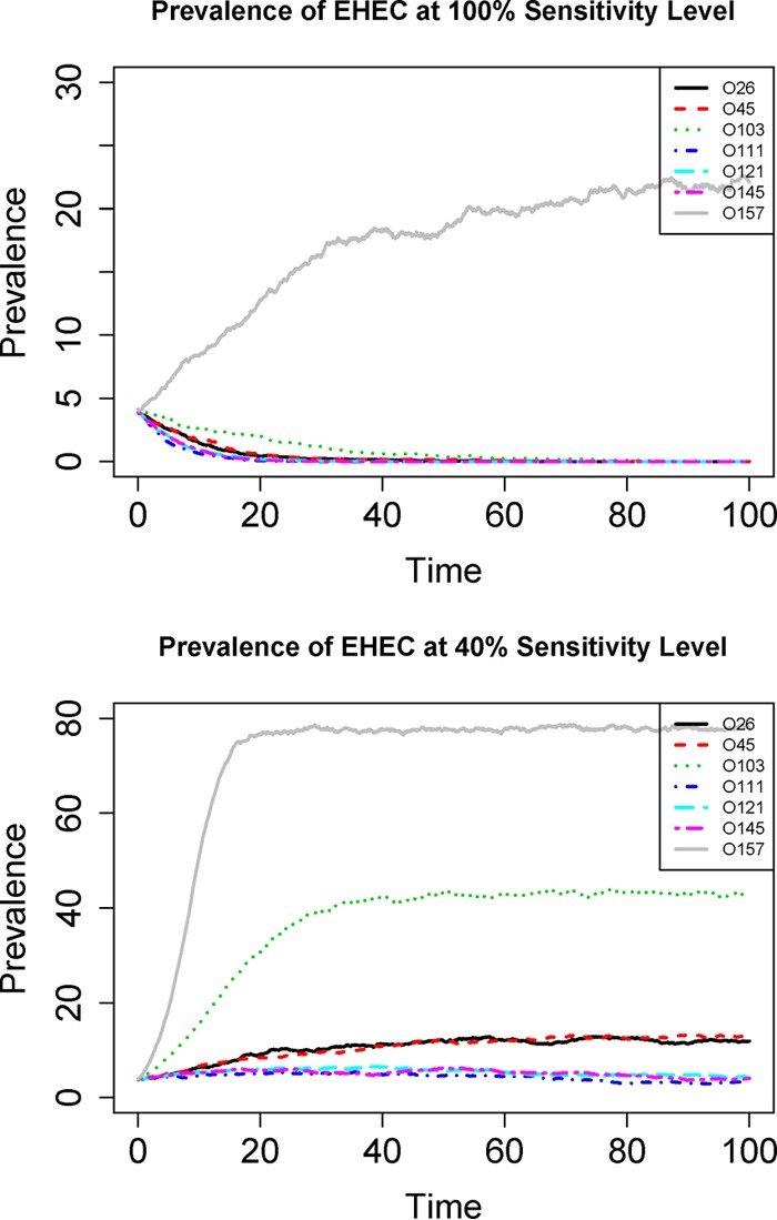
Simulated time series of prevalence for different serogroups using EHEC data at different sensitivity levels. Upper panel, prevalence at 100% detection sensitivity; lower panel, prevalence at 50% detection sensitivity. All the R₀ values are estimated from the 2014 EHEC data. The unit for the x axis is one infectious period (1/γ). Note that the total simulation time is long enough so that even for the O111, O121, and O145 serogroups with R₀ values of >1, the transmissions still eventually die out (lower panel). This is expected from the stochastic Markov model (22).

The R₀ estimates for the seven serogroups from the EHEC data under different sensitivity levels are shown in Fig. 5. The R₀ estimates from the original data are also presented as the baseline (corresponding to a hypothetical 100% sensitivity). At 90% sensitivity (about 10% probability of missing a true case), the R₀ estimates were substantially higher than the baseline estimates; however, still none of the 6 non-O157 serogroups had an R₀ of >1. If the sensitivity level decreased to 75%, then only O103 had an R₀ of >1, and all other non-O157 serogroups (O26, O45, O111, O121, and O145) still had R₀ values of <1. At an even lower sensitivity level (40%), all non-O157 serogroups had R₀ values of >1, although O111, O121, and O145 had R₀ values of marginally greater than one (∼1.10), while O26, O45, and O103 had R₀ values of substantially greater than one. The time series of prevalence using the 40% sensitivity level is provided in Fig. 4 (lower panel) to contrast with the original result (assumed at 100% sensitivity), and the results clearly show that prevalence of O111, O121, and O145 still tended to decrease to zero even though their R₀ values were (marginally) greater than one. This was expected from a stochastic Markov model with absorbing state (22). These results demonstrate the substantial impact of detection sensitivity on estimated R₀ values.

FIG 5.

Estimated R₀ values for serogroups using EHEC data under different sensitivity levels. The error bars represents standard errors associated with the basic reproduction numbers. All six non-O157 serogroups (EHEC data) have R₀ values of <1 at the 100% and 90% sensitivity levels. Only O103 has an R₀ value of >1 at the 75% level, while all other, non-O157 serogroups still have R₀ values of <1 at the 75% level. At the 50% level, all non-O157 serogroups have R₀ values of >1, although O26, O45, and O103 have values substantially larger than one while O111, O121, and O145 have values marginally larger than one.

DISCUSSION

In this study, we estimated the R₀ values of important E. coli serogroups using cross-sectional data with a stochastic Markov chain model. R₀ is one of the most important ecological/epidemiological metrics for infectious pathogens, and the threshold of R₀ (numeric value 1) determines whether the pathogen is able to persist in the population. Furthermore, we also used a Bayesian modeling framework to comprehensively assess the quantitative linkage between multiple external covariates, prevalence, and R₀. Although longitudinal data or multiple cross-sectional data are likely to increase the accuracy of estimates for R₀ (34–36), longitudinal sampling can be financially challenging and infeasible; thus, our approach is very useful under such constraints. We also reconstructed the entire dynamics of prevalence over time (Fig. 3) based on the estimated parameters. Thus, this provides a valuable tool for risk assessment of E. coli burden and enhances our understanding of explicit transmission dynamics of relevant E. coli serogroups on farms (16). Our approach can be easily expanded and adapted to other pathogen systems. The only critical assumption that our approach relies on is that the cross-sectional data are obtained when the system is stationary (steady state). This assumption can be easily met if the pathogen dynamics can be described with a transmission model with only two states (susceptible and infectious), the host population is closed, and the pathogen has a relatively short infectious period (i.e., a large recovery rate γ).

From the results of our model, the R₀ estimates for different serogroups were substantially different, and this result is consistent with previous studies that have estimated R₀ for some of the serogroups (10, 19, 37); only O157 had the potential of persistence in the population because its R₀ was >1. The ability of O157 to specifically colonize the recto-anal junction of cattle is likely to increase the persistence of O157 compared to non-O157 serogroups in the cattle population. O157 has been shown to survive in several environments, including water and soil. Carriage of O157 has also been described in a variety of organisms, including protozoa, invertebrates, birds, and mammals (38). The R₀ values for non-O157 groups were overall lower than that for O157, which suggests that abiotic and biotic reservoirs other than cattle may even play a greater role in non-O157 ecology.

Covariate level-specific R₀ estimates have shown that different serogroups have very different responses to different levels of the covariates (Fig. 3). It is highly possible that current farm conditions favor O157 and provide a better environment for it (and its larger R₀ value would be, indeed, the consequence of such an environment). The lower transmissibility (smaller R₀ value) of other non-O157 serogroups might be the result of less favorable conditions for them (36, 39, 40). We further show that transmissibility for serogroup alone for non-O157 was substantially different than transmissibility of EHEC group. While the O157 serogroup has both Shiga toxin and intimin virulence genes, most non-O157 serogroups modeled here were not associated with virulence genes (9). Thus, the O-group and EHEC data sets were very similar for O157 but different for non-O157 serogroups, where prevalence of EHEC was much lower than for the O-group data, especially for O26, O45, and O103. More specifically, we point out that this study was done during summer months due to financial and labor constraints, and the temperature range in this study is only a subset of potential temperature ranges, which thus warrants further investigation during other seasons as well. In addition, some of the covariate parameter values are close to zero (e.g., the parameters associate with β₄ for all serogroups), which indicated that the corresponding covariate might not influence R₀ substantially.

Our study clearly indicates that different detection sensitivity levels have a substantial impact on estimated propagation capability (as measured by R₀). The transmissibility of non-O157 serogroups is completely different at high sensitivity (100% and 90% sensitivity, approaching disease-free equilibriums for all non-O157 serogroups) than at lower sensitivity (50% sensitivity levels, approaching endemic equilibriums and enabling transmission especially for O26, O45, and O103). Consequently the disease dynamics are completely different. Thus, it is critical to understand test performance for non-O157 serogroup detection and to provide more accurate models of disease dynamics based on accurate R₀ estimates (17, 41).

REFERENCES

- 1.Boyce TG, Swerdlow DL, Griffin PM. 1995. Escherichia coli O157:H7 and the hemolytic-uremic syndrome. N Engl J Med 333:364–368. doi: 10.1056/NEJM199508103330608. [DOI] [PubMed] [Google Scholar]
- 2.Scallan E, Hoekstra RM, Angulo FJ, Tauxe RV, Widdowson MA, Roy SL, Jones JL, Griffin PM. 2011. Foodborne illness acquired in the United States—major pathogens. Emerg Infect Dis 17:7–15. doi: 10.3201/eid1701.P11101. [DOI] [PMC free article] [PubMed] [Google Scholar]
- 3.Erickson M, Doyle M. 2007. Food as a vehicle for transmission of Shiga toxin-producing Escherichia coli. J Food Prot 70:2426–2449. [DOI] [PubMed] [Google Scholar]
- 4.Armstrong GL, Hollingsworth J, Morris JG. 1996. Emerging foodborne pathogens: Escherichia coli O157:H7 as a model of entry of a new pathogen into the food supply of the developed world. Epidemiol Rev 18:29–51. doi: 10.1093/oxfordjournals.epirev.a017914. [DOI] [PubMed] [Google Scholar]
- 5.Rasmussen MA, Casey TA. 2001. Environmental and food safety aspects of Escherichia coli O157:H7 infections in cattle. Crit Rev Microbiol 27:57–73. doi: 10.1080/20014091096701. [DOI] [PubMed] [Google Scholar]
- 6.Elder R, Keen J, Siragusa G, Barkocy-Gallagher G, Koohmaraie M, Laegreid W. 2000. Correlation of enterohemorrhagic Escherichia coli O157 prevalence in feces, hides, and carcasses of beef cattle during processing. Proc Natl Acad Sci U S A 97:2999–3003. doi: 10.1073/pnas.97.7.2999. [DOI] [PMC free article] [PubMed] [Google Scholar]
- 7.Cernicchiaro N, Cull C, Paddock Z, Shi X, Bai J, Nagaraja TG, Renter DG. 2013. Prevalence of Shiga toxin-producing Escherichia coli and associated virulence genes in feces of commercial feedlot cattle. Foodborne Pathog Dis 10:835–841. doi: 10.1089/fpd.2013.1526. [DOI] [PubMed] [Google Scholar]
- 8.Barkocy-Gallagher G, Arthur T, Rivera-Betancourt M, Nou X, Shackelford S, Wheeler T, Koohmaraie M. 2003. Seasonal prevalence of shiga toxin-producing Escherichia coli, including O157:H7 and non-O157 serotypes, and Salmonella in commercial beef processing plants. J Food Prot 66:1978–1986. [DOI] [PubMed] [Google Scholar]
- 9.Dewsbury DA, Renter DG, Shridhar PB, Noll LW, Shi X, Nagaraja TG, Cernicchiaro N. 2015. Summer and winter prevalence of STEC O26, O45, O103, O111, O121, O145, and O157 in feces of feedlot cattle. Foodborne Pathog Dis 12:726–732. doi: 10.1089/fpd.2015.1987. [DOI] [PubMed] [Google Scholar]
- 10.Liu WC, Shaw DJ, Matthews L, Hoyle DV, Pearce MC, Yates CM, Lows JC, Amyes SGB, Gunn GJ, Woolhouse MEJ. 2007. Modelling the epidemiology and transmission of verocytotoxin-producing Escherichia coli serogroups O26 and O103 in two different calf cohorts. Epidemiol Infect 135:1316–1323. [DOI] [PMC free article] [PubMed] [Google Scholar]
- 11.Anderson R, May R. 1992. Infectious disease in humans. Oxford University Press, Oxford, United Kingdom. [Google Scholar]
- 12.Paaijmans KP, Read AF, Thomas MB. 2009. Understanding the link between malaria and climate. Proc Natl Acad Sci U S A 106:13844–13849. doi: 10.1073/pnas.0903423106. [DOI] [PMC free article] [PubMed] [Google Scholar]
- 13.Chen S, Fleischer SJ, Saunders MC, Thomas MB. 2015. The influence of diurnal temperature variation on degree-day accumulation and insect life history. PLoS One 10:e0120772. doi: 10.1371/journal.pone.0120772. [DOI] [PMC free article] [PubMed] [Google Scholar]
- 14.Jacob ME, Paddock ZD, Renter DG, Lechtenberg KF, Nagaraja TG. 2010. Inclusion of dried or wet distiller's grains at different levels in diets of feedlot cattle affects fecal shedding of Escherichia coli O157:H7. Appl Environ Microbiol 76:7238–7242. doi: 10.1128/AEM.01221-10. [DOI] [PMC free article] [PubMed] [Google Scholar]
- 15.Cull CA, Paddock ZD, Nagaraja TG, Bello NM, Babcock AH, Renter DG. 2012. Efficacy of a vaccine and a direct-fed microbial against fecal shedding of Escherichia coli O157:H7 in a randomized pen-level field trial of commercial feedlot cattle. Vaccine 30:6210–6215. doi: 10.1016/j.vaccine.2012.05.080. [DOI] [PubMed] [Google Scholar]
- 16.Chen S, Sanderson M, Lanzas C. 2013. Investigating effects of between- and within-host variability on Escherichia coli O157 shedding pattern and transmission. Prev Vet Med 109:47–57. doi: 10.1016/j.prevetmed.2012.09.012. [DOI] [PubMed] [Google Scholar]
- 17.Hefferman JM, Smith RJ, Wahl LM. 2005. Perspectives on the basic reproductive ratio. J R Soc Interface 2:281–293. doi: 10.1098/rsif.2005.0042. [DOI] [PMC free article] [PubMed] [Google Scholar]
- 18.Zuur A, Ieno EN, Smith GM. 2007. Analysing ecological data. Springer, New York, NY. [Google Scholar]
- 19.Matthews L, McKendreick IJ, Ternet H, Gunn GJ, Synge B, Woolhouse MEJ. 2006. Super-shedding cattle and the transmission dynamics of Escherichia coli O157. Epidemiol Infect 134:131–142. [DOI] [PMC free article] [PubMed] [Google Scholar]
- 20.Matthews L, Reeve R, Woolhouse MEJ, Chase-Topping M, Mellor DJ, Pearce MC, Allison LJ, Gunn GJ, Low JC, Reid SWJ. 2009. Exploiting strain diversity to expose transmission heterogeneities and predict the impact of targeting supershedding. Epidemics 1:221–229. doi: 10.1016/j.epidem.2009.10.002. [DOI] [PubMed] [Google Scholar]
- 21.O'Reilly KM, Low JC, Denwood MJ, Gally DL, Evans J, Gunn GJ, Mellor DJ, Reid SWJ, Matthews L. 2010. Associations between the presence of virulence determinants and the epidemiology and ecology of zoonotic Escherichia coli. Appl Environ Microbiol 76:8110–8116. doi: 10.1128/AEM.01343-10. [DOI] [PMC free article] [PubMed] [Google Scholar]
- 22.Allen LJS, Allen EJ. 2003. A comparison of three different stochastic population models with regard to persistence time. Theor Popul Biol 64:439–449. doi: 10.1016/S0040-5809(03)00104-7. [DOI] [PubMed] [Google Scholar]
- 23.Nasell I. 1996. The quasi-stationary distribution of the closed endemic SIS model. Adv Appl Prob 28:895–932. doi: 10.2307/1428186. [DOI] [Google Scholar]
- 24.Nasell I. 2001. Extinction and quasi-stationarity in the stochastic logistic SIS model. Springer, New York, NY. [DOI] [PubMed] [Google Scholar]
- 25.Clancy D, O'Neil PD. 2008. Bayesian estimation of the basic reproduction number in stochastic epidemic models. Bayesian Anal 3:737–758. doi: 10.1214/08-BA328. [DOI] [Google Scholar]
- 26.Hall DB. 2000. Zero-inflated Poisson and binomial regression with random effects: a case study. Biometrics 56:1030–1039. doi: 10.1111/j.0006-341X.2000.01030.x. [DOI] [PubMed] [Google Scholar]
- 27.Gosh SK, Mukhopadhyay P, Lu JC. 2006. Bayesian analysis of zero-inflated regression models. J Stat Plan Infer 136:1360–1375. doi: 10.1016/j.jspi.2004.10.008. [DOI] [Google Scholar]
- 28.Martin TG, Wintle BA, Rhodes JR, Kuhnert PM, Field SA, Low-Choy SJ, Tyre AJ, Possingham HP. 2005. Zero tolerance ecology: improving ecological inference by modeling the source of zero observations. Ecol Lett 8:1235–1246. doi: 10.1111/j.1461-0248.2005.00826.x. [DOI] [PubMed] [Google Scholar]
- 29.Echeverry A, Loneragan GH, Wagner BA, Brashears MM. 2005. Effect of intensity of fecal pat sampling on estimates of Escherichia coli O157 prevalence. Am J Vet Res 66:2023–2027. doi: 10.2460/ajvr.2005.66.2023. [DOI] [PubMed] [Google Scholar]
- 30.Branscum AJ, Gardner IA, Johnson WO. 2004. Bayesian modeling of animal- and herd-level prevalences. Prev Vet Med 66:101–112. doi: 10.1016/j.prevetmed.2004.09.009. [DOI] [PubMed] [Google Scholar]
- 31.Clough HE, Clancy D, O'Neill PD, French NP. 2003. Bayesian methods for estimating pathogen prevalence within groups of animals from faecal-pat sampling. Prev Vet Med 58:145–169. doi: 10.1016/S0167-5877(03)00050-3. [DOI] [PubMed] [Google Scholar]
- 32.Conrad CC, Stanford K, McAllister TA, Thomas J, Reuter T. 2014. Further development of sample preparation and detection methods for O157 and the top 6 non-O157 STEC serogroups in cattle feces. J Microbiol Methods 105:22–30. doi: 10.1016/j.mimet.2014.06.020. [DOI] [PubMed] [Google Scholar]
- 33.Rogan WJ, Gladen B. 1978. Estimating prevalence from the results of a screening test. Am J Epidemiol 107:71–76. [DOI] [PubMed] [Google Scholar]
- 34.Ray KJ, Porco TC, Hong KC, Lee DC, Alemayehu W, Melese M, Lakew T, Yi E, House J, Chidambaram JD, Whitcher JP, Gaynor BD, Lietman TM. 2007. A rationale for continuing mass antibiotic distribution for trachoma. BMC Infect Dis 7:91. doi: 10.1186/1471-2334-7-91. [DOI] [PMC free article] [PubMed] [Google Scholar]
- 35.Ray KJ, Lietman TM, Porco TC, Keen JD, Bailey RL, Solomon AW, Burton MJ, Harding-Esch E, Holland MJ, Mabey D. 2009. When can antibiotic treatments for trachoma be discontinued? Graduating communities in three African countries. PLoS Negl Trop Dis 3:e458. doi: 10.1371/journal.pntd.0000458. [DOI] [PMC free article] [PubMed] [Google Scholar]
- 36.Herbert LJ, Vali L, Hoyle DV, Innocent G, McKendreick IJ, Pearce MC, Mellor D, Porphyre T, Locking M, Allison L, Hanson M, Matthews L, Gunn GJ, Woolhouse MEJ. 2014. E.coli O157 on Scottish cattle farms: evidence of local spread and persistence using repeat cross-sectional data. BMC Vet Res 10:95. doi: 10.1186/1746-6148-10-95. [DOI] [PMC free article] [PubMed] [Google Scholar]
- 37.Chandran A, Hatha AA, Varghese S, Sheeja KM. 2008. Prevalence of multiple drug resistant Escherichia coli serotypes in a tropical estuary, India. Microbes Environ 23:153–158. doi: 10.1264/jsme2.23.153. [DOI] [PubMed] [Google Scholar]
- 38.Besser TE, Schmidt CE, Shah DH, Shringi S. 2014. “Preharvest” food safety for Escherichia coli O157 and other pathogenic Shiga toxin-producing strains. Microbiol Spectrum 2(5):EHEC-0021-2013. doi: 10.1128/microbiolspec.EHEC-0021-2013. [DOI] [PubMed] [Google Scholar]
- 39.Muffling T, Smaijlovic M, Nowak B, Sammet K, Bulte M, Klein G. 2007. Preliminary study of certain serotypes, genetic, and antimicrobial resistance profiles of verotoxigenic Escherichia coli (VTEC) isolated in Bosnia and Germany from cattle or pigs and their products. Int J Food Microbiol 117:185–191. doi: 10.1016/j.ijfoodmicro.2006.08.003. [DOI] [PubMed] [Google Scholar]
- 40.Scott L, McGee P, Walsh C, Fanning S, Sweeney T, Blanco J, Karczmarczyk M, Early B, Leonard N, Sheridan JJ. 2009. Detection of numerous verotoxigenic E. coli serotypes, with multiple antibiotic resistance from cattle faeces and soil. Vet Microbiol 134:288–293. doi: 10.1016/j.vetmic.2008.08.008. [DOI] [PubMed] [Google Scholar]
- 41.Samsuzzoha M, Sigh M, Lucy D. 2013. Uncertainty and sensitivity analysis of the basic reproduction number of a vaccinated epidemic model of influenza. Appl Math Model 37:903–915. doi: 10.1016/j.apm.2012.03.029. [DOI] [Google Scholar]
- 42.Noll LW, Baumgartner WC, Shridhar PB, Cull CA, Dewsbury DM, Shi X, Cernicchiaro N, Renter DG, Nagaraja TG. 2016. Pooling of immunomagnetic separation beads does not affect detection sensitivity of six major serogroups of Shiga toxin-producing Escherichia coli in cattle feces. J Food Prot 7:59–65. doi: 10.4315/0362-028X.JFP-15-236. [DOI] [PubMed] [Google Scholar]
Associated Data
This section collects any data citations, data availability statements, or supplementary materials included in this article.