Assessment of blood flow velocity and pulsatility in cerebral perforating arteries with 7‐T quantitative flow MRI

Abstract

Thus far, blood flow velocity measurements with MRI have only been feasible in large cerebral blood vessels. High‐field‐strength MRI may now permit velocity measurements in much smaller arteries. The aim of this proof of principle study was to measure the blood flow velocity and pulsatility of cerebral perforating arteries with 7‐T MRI. A two‐dimensional (2D), single‐slice quantitative flow (Qflow) sequence was used to measure blood flow velocities during the cardiac cycle in perforating arteries in the basal ganglia (BG) and semioval centre (CSO), from which a mean normalised pulsatility index (PI) per region was calculated (n = 6 human subjects, aged 23–29 years). The precision of the measurements was determined by repeated imaging and performance of a Bland–Altman analysis, and confounding effects of partial volume and noise on the measurements were simulated. The median number of arteries included was 14 in CSO and 19 in BG. In CSO, the average velocity per volunteer was in the range 0.5–1.0 cm/s and PI was 0.24–0.39. In BG, the average velocity was in the range 3.9–5.1 cm/s and PI was 0.51–0.62. Between repeated scans, the precision of the average, maximum and minimum velocity per vessel decreased with the size of the arteries, and was relatively low in CSO and BG compared with the M1 segment of the middle cerebral artery. The precision of PI per region was comparable with that of M1. The simulations proved that velocities can be measured in vessels with a diameter of more than 80 µm, but are underestimated as a result of partial volume effects, whilst pulsatility is overestimated. Blood flow velocity and pulsatility in cerebral perforating arteries have been measured directly in vivo for the first time, with moderate to good precision. This may be an interesting metric for the study of haemodynamic changes in aging and cerebral small vessel disease. © 2015 The Authors NMR in Biomedicine Published by John Wiley & Sons Ltd.

Abbreviations used

2D/3D

two‐/three‐dimensional

BG

basal ganglia

CI

confidence interval

CSO

semioval centre

CoR

coefficient of repeatability

ICC

intraclass correlation coefficient

PI

pulsatility index

Qflow

quantitative flow

RF

radiofrequency

ROI

region of interest

SD

standard deviation

SNR

signal‐to‐noise ratio

V_mean

average velocity

V_max

maximum velocity

V_min

minimum velocity

WM

white matter.

Introduction

The brain is a high‐flow, low‐impedance organ, and therefore sensitive to the effects of increased arterial blood flow pulsatility 1. High carotid artery blood flow pulsatility is associated with microvascular structural brain damage and lower scores in various cognitive domains 2, 3, 4, 5. Increased blood flow pulsatility is also associated with microcirculatory remodelling 6 and could represent a mechanistic link between aortic stiffening, brain lesions and cognitive impairment 2. However, direct assessment of blood flow velocity and pulsatility in human cerebral perforating arteries and arterioles in vivo has not been possible thus far. The diameters of perforating arteries in the semioval centre (CSO) range from approximately 10 to 300 µm 7, 8 and, because of this small size and relatively slow blood flow velocity, even the mere depiction of cerebral penetrating arteries is challenging with time‐of‐flight MRI. With the advent of 7‐T MRI, various reports have shown the feasibility of the depiction of the relatively large perforating arteries in the basal ganglia (BG) 9, 10, 11, 12, 13. Recently, cerebral perforating arteries in CSO were visualised for the first time with 7‐T MRI 14. Given the relatively long T ₂* of arterial blood, we hypothesised that it might also be possible to assess the velocity and pulsatility in cerebral perforating arteries with phase contrast MRI. This could provide an important new metric for the study of the haemodynamics in these vessels, and their association with, for example, vascular lesions or cognitive impairment.

Therefore, the aim of this study was to measure the velocity and pulsatility of blood flow in cerebral perforating arteries in the brain with 7‐T phase contrast velocity mapping MRI. After empirical optimisation of a two‐dimensional (2D) quantitative flow (Qflow) sequence to measure slow‐flowing blood velocities in small arteries, six human volunteers were scanned. The velocity and pulsatility in penetrating arteries were measured in CSO and BG. The precision of the measurements was determined, and potentially confounding effects of partial volume and noise on the measurements in CSO were estimated with simulations.

Methods

Study design

Six volunteers were scanned twice on the same day on a 7‐T MRI scanner. Blood flow velocities were measured in: (i) the perforating medullary arteries in CSO; and (ii) the lenticulostriate arteries at the level of BG. As a frame of reference, the blood flow velocity was also measured in the proximal M1 segment of the middle cerebral artery.

For each vessel, we recorded the average (V _mean), maximum (V _max) and minimum (V _min) velocities during the cardiac cycle. A pulsatility index (PI) per anatomical region was calculated, using the average normalised velocity over all vessels to construct an average normalised velocity curve, from which PI was derived:

$$\text{PI}=\frac{\left({\mathit{V}}_{\text{max}}-{\mathit{V}}_{\text{min}}\right)}{{\mathit{V}}_{\text{mean}}}$$ (1)

The precision of the velocity measurements in individual vessels and the PI per anatomical region were determined. Because the diameters of the penetrating arteries in CSO were smaller than our voxel size, the potentially confounding effects of partial volume on the measured velocities were estimated with simulations, taking into account the vessel diameter, voxel size, noise and the slice profile of the radiofrequency (RF) excitation pulse used.

The study was approved by the Ethical Review Board of our hospital, and all volunteers gave written informed consent prior to their participation.

Image acquisition

Six volunteers (four women and two men), aged 23–29 years, were scanned on a 7‐T MRI scanner (Philips Healthcare, Cleveland, OH, USA) using a volume transmit coil and a 32‐channel receive coil (Nova Medical, Wilmington, MA, USA). The MRI protocol consisted of a retrospectively gated 2D phase contrast Qflow sequence (field of view, 250 × 180 mm²) with the following parameters: acquired voxel size, 0.3 × 0.3 × 2.0 mm³; TR/TE = 26/15 ms; flip angle, 60°; readout bandwidth, 59 Hz/pixel [to increase the signal‐to‐noise ratio (SNR) of arterial blood, which has a long T ₂* of approximately 32 ms at 7 T (estimated with a multi‐echo gradient echo sequence in a single subject)]; V _enc, velocity encoding (Venc) 4 and 20 cm/s for CSO and BG, respectively; two averages; 10–13 reconstructed heart phases (true temporal resolution, 156 ms); scan duration, approximately 7 min. To minimise motion of the head, cushions were placed beside the head of the person who was scanned.

Compared with a standard clinical 2D Qflow sequence, the main differences in parameters are the high flip angle to minimise partial volume effects by suppressing the background signal, the high in‐plane resolution and the long TE in combination with a low bandwidth, which are possibly a result of the slow flow in the small vessels (yielding less sensitivity to flow effects) and the relatively long T ₂* of arterial blood (relative to venous blood).

For M1, a similar Qflow sequence with the following parameters was used: field of view, 250 × 200 mm²; acquired voxel size, 0.5 × 0.5 × 2.0 mm³; TR/TE, 18/7.6 ms; flip angle, 60°; readout bandwidth, 126 Hz/pixel; V _enc, 100 cm/s; 15 reconstructed heart phases; true temporal resolution, 111 ms; scan duration, approximately 2 min. A peripheral pulse unit on the left ring, middle or index finger was used for synchronisation with the heart cycle.

Further, a three‐dimensional (3D) T ₁‐weighted sequence with an isotropic resolution of 1.0 mm and whole brain coverage was acquired to plan the 2D Qflow imaging planes, and 2D T ₂‐weighted turbo spin echo (TR/TE = 2000/74 ms; resolution, 0.4 × 0.4 × 2.0 mm³) images were acquired as anatomical reference at the same levels as the 2D Qflow slices. The 2D Qflow acquisition was planned manually, as follows. Two single transverse slices were planned on sagittal images of the T ₁‐weighted sequence: (i) at the level of BG, through the anterior commissure, parallel to the genu and splenium of the corpus callosum; and (ii) through CSO, approximately 15 mm above the top of the corpus callosum (Fig. 1A). In M1, either the left or right proximal artery was chosen depending on which offered the best planning perpendicular to the vessel orientation. The 2D Qflow slice was planned perpendicular to the proximal M1 artery, using transverse and coronal maximum intensity projections of the T ₁‐weighted images.

Figure 1.

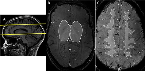
Planning of the two‐dimensional (2D) quantitative flow (Qflow) slices and regions of interest (ROIs). (A) Planning of the basal ganglia (BG) and semioval centre (CSO) slices on a sagittal T ₁‐weighted image. The slice planning is indicated by the yellow lines. (B) ROI on the 2D Qflow image in the BG slice. (C) ROI on the 2D Qflow image in the CSO slice. A relatively narrow ROI was used that excluded juxtacortical white matter (WM) to avoid counting vessels from sulci beneath the slice as penetrating arteries.

Subjects were scanned twice on the same day with 15 min between the two scan sessions, and were repositioned before the second session. To be able to analyse the precision of the velocities in individual vessels, and to evaluate as much as possible the precision of the measurements (and not physiology or anatomy), the location and orientation of the 2D Qflow slices in the second scan had to be as similar as possible to those of the first scan. Therefore, the 2D Qflow slices of the second scan were automatically planned, using the automatic planning feature provided by the scanner 15. The automatic planning feature of the scanner used the T ₁‐weighted images of scan session 2 (which were acquired before planning the 2D Qflow slices) and registered these images to the T ₁ images acquired during the first scan session. After this, the scanner automatically planned the 2D Qflow slices of session 2, by transforming the coordinates of the 2D Qflow slices of session 1 to session 2, with respect to the anatomical reference as given by the T ₁ scan.

Image processing

We used an in‐house‐developed tool employing MeVisLab software (MeVis Medical Solutions AG, Bremen, Germany) 16 to analyse the 2D Qflow images. Briefly, this included the following steps.

1. Phase correction of the velocity measurements by estimating the background phase offset from the mean (over the cardiac cycle) phase image, using a median filter (size 21 × 21 pixels), and subtracting the background phase from the phase images of each cardiac time point.

2. Estimation of the SNR of the velocity measurements by calculating its standard deviation (SD) (σ_v) from the SNR of the magnitude images (SNR_mag) as follows:

$${\sigma }_v=\frac{V_{enc}}{\pi }\frac{1}{{\mathrm{S}\mathrm{N}\mathrm{R}}_{mag}}$$ (2)

SNR_mag was estimated pixelwise from the magnitude image (signal) and the SD of the real and imaginary parts of the signal over the cardiac phases (as a measure of noise, which was median filtered (21 × 21) before calculating a pixelwise SNR_mag map). Noise was estimated on a pixel‐by‐pixel basis from the noise fluctuations over the cardiac cycle. It was assumed that the signal was stable over the cardiac cycle, and that any signal variation over the heart cycle was noise.A mask was created to simplify the identification of vessels. All voxels with significant flow were included in the mask: voxels in which the 95% confidence interval (CI) of the velocity (based on 2σ_v) included zero at any time point of the cardiac cycle were masked out. Potential vessels obtained from this mask were indicated by squares on the 2D Qflow magnitude image, as indicated in Fig. 2. As this step yielded many more potential vessels than could be readily confirmed, we performed a manual identification of vessels.

• Manual identification of vessels within a region of interest (ROI) that was drawn on each 2D Qflow slice (Fig. 1B, C). For BG, the anterior, posterior and lateral border zones of the ROI were defined at the anterior end of the insula, the posterior end of the thalamus and the claustrum, respectively. For CSO, the ROI was defined by the white matter (WM) that did not show obvious partial volume effects with non‐WM tissue on any of the acquisitions (T ₁, T ₂, cumulative magnitude). Voxels that were identified in step 2, and had a round, delineable hyperintensity on the cumulative images at the same coordinates, were identified as an artery (Fig. 2), provided that they were visible on both scans 1 and 2. A single voxel was selected per vessel, because of the subvoxel diameters of these vessels. Potential vessels were excluded if they were located within ghosting artefacts caused by larger arteries, or were clearly not orthogonal to the slice.

Figure 2.

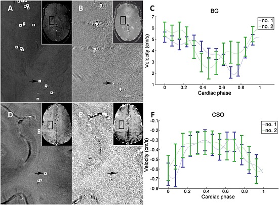
Vessel selection and raw data example. (A–C) Basal ganglia (BG). (D–F) Semioval centre (CSO). (A, D) Mean magnitude images over all 13 cardiac time points. (B, E) Mean phase images. (C, F) Raw data curves for the measurement of velocity for the individual vessels indicated with the black arrows. All images are of volunteer 1. Local maxima in mean velocity are indicated with white squares on the magnitude images. Note that some local maxima are not located within a corresponding artery on the magnitude images (these were excluded). The black arrows point to the vessels for which the velocity profiles are shown as an example of our raw data in (C) and (F). Note that the blood flow direction of the perforating arteries in CSO is opposite to that of the arteries in BG, which can be observed from the negative values of the CSO velocity curve (F) and the hypointense appearance of arteries in the CSO phase image (E), which is caused by the direction of flow. The error bars show ± standard deviation of the estimated noise [Equation 2] at the location of the measurement. The connecting lines are interpolated. The blue lines indicate measurement 1 and the green lines the repeated measurement after repositioning of the subject.

The reference vessels (M1) were analysed on site with the scanner software instead of the developed MeVisLab tool. An ROI was drawn in the M1 segments, within which the mean blood velocity per cardiac phase was calculated.

Velocity curve analysis

For each vessel, V _mean, V _max and V _min were recorded. The calculation of PI per vessel proved to be very sensitive to noise, and so PI was calculated per region from the mean normalised velocity curve over all vessels in the corresponding region. These mean normalised velocity curves per region were constructed as follows: first, the velocity curve of each vessel was normalised by dividing it by its mean velocity to obtain the same weighting of vessel with high and low velocities; second, the mean normalised velocity over all vessels per time point was taken to plot the normalised velocity curve per region, and PI was calculated from this curve.

To explore the differences in blood flow velocity and pulsatility between the penetrating arteries in CSO, BG and M1, a mean normalised velocity curve of all volunteers combined was created for each region. To be able to combine the mean normalised velocity curves of the volunteers, different numbers of sample points (as a result of differences in heart rate) and different time lags of the curves with respect to the cardiac cycle (as a result of the different distances blood travels in each volunteer between the heart and the peripheral pulse unit, and between the heart and the cerebral vasculature) had to be synchronised. Therefore, all velocity curves with less than 13 sample points were interpolated to 13 sample points (using Fourier interpolation), which was the maximum number of sample points in CSO and BG. To synchronise the difference in time lags with respect to the cardiac cycles, the time lag between each volunteer's M1 velocity curve and the mean M1 velocity curve over all volunteers was removed from each volunteer's curve. After this, a mean normalised curve over all volunteers was created. All processing of the velocity curves was performed in MATLAB (MATLAB 8.3, The MathWorks Inc., Natick, MA, USA, 2014).

Simulations

Simulations were performed to confirm that the measured velocities in the perforating medullary arteries were consistent with the known velocities and diameters of small vessels (i.e. based on the physiological properties of small artery flow as reported in the literature), if confounding factors, such as noise and partial volume effects, are taken into account. As a result of the influence of partial volume effects and noise, the estimated velocities of the flow in small arteries in the WM might be different from the true velocities. Given a vessel with a diameter d smaller than the voxel size and a certain velocity v, the estimated velocity obtained from the MRI phase contrast signal was simulated. The simulations were performed for a vessel perpendicular to the imaging plane, assuming that the entire lumen falls within a single voxel. The effect of the blood velocity profile was not incorporated into the simulations. For a parabolic velocity slice profile in a subvoxel vessel, as simulated here, it can be shown that the phase of the phase contrast MRI signal yields the mean velocity, if no signal from static surrounding tissue is present (see Appendix S1). Hence, plug flow was assumed, with the velocity representing the mean velocity of the blood velocity profile.

The simulations were performed for a range of vessel diameters (50–300 µm, in 250 steps) and a range of velocities (5–40 mm/s, in 250 steps) for the voxel size (300 µm) and flip angle (60°) used in the imaging protocol. The flip angle slice profile was calculated using the Bloch equations, and employed in the simulations by applying the approach described by Matsuda et al. 17. Straightforward numerical computations of the static tissue and blood signal (including time‐of‐flight effects) were performed, based on the Bloch equations and using T ₁/T ₂* = 2100/32 ms for blood and 1200/27 ms for brain tissue (WM) 18, 19, 20. The effect of noise was simulated using a Monte Carlo approach. The SNR of static tissue without a blood vessel was set to 7, based on an estimation of the SNR in the acquired images. The estimated velocity and SD as a result of noise were obtained, and the region of velocity–diameter combinations for which the estimated velocity was significantly larger than zero (i.e. larger than 2SD) was indicated.

Literature values of the relation between vessel diameter and blood velocity were added to the plot obtained from the simulations. Kobari et al. 21 reported centreline velocities (v _c) in feline pial arteries, and provided the following equation for the velocity as a function of the diameter (in µm): v _c = (0.34d + 0.309) (mm/s).

Further, results were taken from Nagaoka et al. 22, who measured arterial velocities over the cardiac cycle in two arterioles (approximately 100 µm in diameter) of the human retina. To correct for the fact that both references use centreline velocities, whereas we measure approximately the mean velocity, a conversion factor of 1.58 was employed between the centreline velocity and mean velocity. This conversion factor was taken from equation 4 in Koutsiaris et al. 23, given that the vessel diameters are much larger than the red blood cell diameter. The simulations were performed using MATLAB (MATLAB 8.3, The MathWorks Inc., Natick, MA, USA, 2014).

Statistical analysis

Correlations were tested with Spearman's rank correlation tests. The precision of the measurements between repeated scans was evaluated by a Bland–Altman analysis. A coefficient of repeatability (CoR) was calculated to evaluate the level of agreement between repeated scans. CoR was defined as: (square root of the mean squared difference between scan 1 and scan 2) × 1.96 24. For the mean curves per region, the standard error of the mean and corresponding 95% CIs were calculated.

Results

Blood flow velocities and PI

The image post‐processing (step 2) yielded a median of 53 potential vessels per subject for CSO (range, 24–102) and a median of 86 for BG (range, 46–115). After manual identification, the median number of vessels that were included was 14 in CSO (range, 5–20) and 19 in BG (range, 7–25). An example of a blood flow velocity curve of an individual artery is shown in Fig. 2. V _mean (i.e. the mean velocity across a cardiac cycle) was calculated for each individual vessel. The distribution of the V _mean values per vessel in each subject is displayed in Fig. 3. Across subjects, the average V _mean across vessels was in the range 0.5–1.0 cm/s in CSO and 3.9–5.1 cm/s in BG (Table 1).

Figure 3.

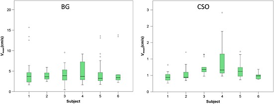
Boxplots showing the distribution of the average velocity of individual blood vessels for each subject. The number of vessels per subject is displayed in Table 1. Note that little between‐subject variability is seen in the median average velocity in the basal ganglia (BG), despite considerable variability in the range of velocities that were measured within subjects. In the semioval centre (CSO), more variability in the median average velocity was observed compared with BG.

Table 1.

Subject characteristics, blood flow velocities and pulsatility index (PI). For each vessel, V _mean was recorded, which is the mean velocity during the cardiac cycle. The average V _mean ± standard deviation (SD) in each region and per volunteer is displayed. The PI per region was derived from the normalised velocity curve over all vessels in that region. For each region, the entire region of interest was analysed, which means that vessels from both hemispheres were combined

			Semioval centre			Basal ganglia
Subject	Age (years)	Sex	N a	V mean (cm/s) ± SD	PI	N a	V mean (cm/s) ± SD	PI
1	29	F	20	0.46 ± 0.13	0.26	20	5.1 ± 4.0	0.51
2	26	F	15	0.55 ± 0.23	0.25	7	3.9 ± 1.3	0.38
3	28	F	8	0.87 ± 0.28	0.39	17	4.1 ± 2.2	0.48
4	28	M	13	1.03 ± 0.61	0.39	19	4.9 ± 2.6	0.47
5	23	M	14	0.70 ± 0.25	0.24	25	4.7 ± 2.6	0.32
6	25	F	5	0.49 ± 0.12	0.26	6	5.0 ± 4.3	0.46

^a N, number of vessels analysed in the corresponding region.

PI was derived from the mean normalised velocity curve over all vessels in the corresponding region. Examples of these mean normalised velocity curves are shown in Fig. 4. PI was in the range 0.24–0.39 in CSO and 0.32–0.51 in BG (Table 1).

Figure 4.

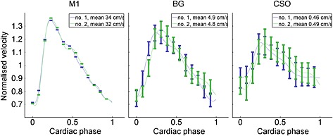
Example of normalised velocity curves of the first and second scans. Data shown from volunteer 1. Error bars show ± standard error of the mean over all vessels in the respective area. Because there was only one measurement for the M1 segment of the middle cerebral artery (M1), no error bars are shown. The connecting lines are interpolated. For visualisation purposes, the samples of all curves were shifted to show the minimum of M1 as the first point in the cardiac cycle. The blue lines indicate the mean normalised velocity curves per region for measurement 1 of all vessels, and the green curves show measurement 2. BG, basal ganglia; CSO, semioval centre.

Precision of the velocity measurements

V _mean and V _max showed a strong correlation in CSO [intraclass correlation coefficient (ICC), 0.76 and 0.79, respectively], and excellent correlation between repeated scans in BG (ICC, 0.86 for both). Bland–Altman plots show the agreement of V _mean and V _max between repeated scans (Fig. 5). No systematic errors were observed, but the 95% limits of agreement are relatively wide compared with the mean velocity. The mean absolute difference ± SD of V _mean between repeated scans was 0.14 ± 0.15 cm/s (relative to the average V _mean: 23% ± 23%) in CSO, and 0.66 ± 0.72 cm/s (relative to the average V _mean: 14% ± 16%) in BG. The CoRs of V _mean and V _max relative to the average V _mean are much larger in BG and CSO relative to M1 (Table 2).

Figure 5.

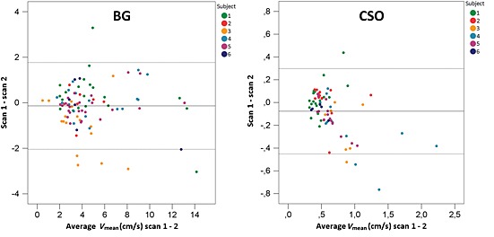
Bland–Altman plots showing the agreement of V _mean per vessel between repeated scans. The broken lines indicate the upper and lower limits of agreement and the full line the mean difference between scans 1 and 2. BG, basal ganglia; CSO, semioval centre.

Table 2.

Coefficients of repeatability (CoR) of blood flow velocities and pulsatility index

Region	V mean (cm/s)		V max (cm/s)		V min (cm/s)		Pulsatility indexa
	Average	CoR (%)	Average	CoR (%)	Average	CoR (%)	Average	CoR (%)
CSO	0.63 ± 0.19	0.46/73	0.82 ± 0.19	0.46/56	0.44 ± 0.16	0.47/107	0.28 ± 0.07	0.14/50
BG	4.6 ± 0.64	1.9/41	5.7 ± 0.91	2.1/37	3.3 ± 0.45	2.1/62	0.40 ± 0.09	0.15/38
M1	42 ± 8.0	10/24	55 ± 9.1	15/27	32 ± 6.8	9.6/30	0.56 ± 0.09	0.24/43

^aThe pulsatility index (PI) is defined in Equation 1, and was derived from the normalised velocity curve over all vessels per region, per individual.

For V _mean, V _max, V _min and PI, the average value ± standard deviation (SD) of all subjects combined is displayed in the left column (determined per individual, and then averaged over all individuals). In the right column, the coefficient of repeatability is displayed as an absolute value (left) and relative to the average of all individuals (right).

BG, basal ganglia; CSO, semioval centre; M1, M1 segment of the middle cerebral artery; V _mean, V _max, V _min, mean, maximum and minimum velocity during the cardiac cycle, determined per vessel.

Precision of PI

Bland–Altman plots show the agreement of PI per region between repeated scans (Fig. 6). As a frame of reference, the repeatability of the measurements in M1 is also displayed. No systematic errors were observed. The mean absolute difference ± SD of PI between repeated scans was 0.09 ± 0.03 (relative to mean PI, 32% ± 9%) in CSO and 0.07 ± 0.07 (relative to mean PI, 18% ± 17%) in BG. The CoRs of PI in CSO and BG are of similar size to that in M1 (Table 2).

Figure 6.

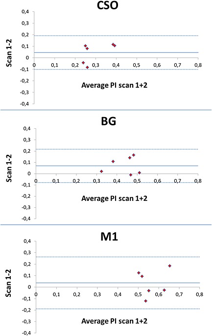
Bland–Altman plots showing the agreement of the pulsatility index (PI) between repeated scans. The broken lines indicate the upper and lower limits of agreement and the full line the mean difference between scans 1 and 2. BG, basal ganglia; CSO, semioval centre; M1, M1 segment of the middle cerebral artery.

Mean normalised velocity curves of all volunteers combined

The average mean normalised velocity curves over all subjects show a decrease in PI from M1 to the perforating arteries in BG and CSO (Fig. 7). At the peaks of the curves, the error bars of CSO, BG and M1 areas do not overlap, showing a significant difference in normalised velocity. Furthermore, a small time lag between the different regions was observed, as would be expected.

Figure 7.

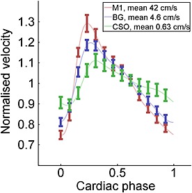
Average normalised velocity profiles over all vessels of all volunteers combined, shown per area. Error bars show ± standard error of the mean. The connecting lines are interpolated. The pulsatility (difference between the maximum and minimum normalised velocity) is highest in M1, and lowest in CSO. BG, basal ganglia; CSO, semioval centre; M1, M1 segment of the middle cerebral artery.

Simulations

Fig. 8 shows the estimated velocity map as a function of the true velocity. It appears that the area with detectable velocity–diameter combinations contains physiologically realistic values, and that the smallest vessels that can be detected have a diameter of around 80 µm. However, the velocities are considerably underestimated for vessels with diameters much smaller than the in‐plane resolution of the image (300 µm). Somewhat unexpectedly, the underestimation of the velocities does not lead to an underestimation of PI. Instead, PI is overestimated, as illustrated in Fig. 8B.

Figure 8.

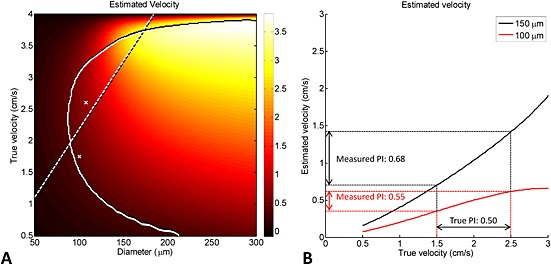
Simulation showing the estimated velocity map as a function of the true velocity. (A) Simulation results showing the estimated velocity as a function of the true blood velocity and vessel diameter for the scan protocol parameters used in the semioval centre (CSO): slice thickness, 2 mm; in‐plane resolution, 300 µm; flip angle, 60°; static tissue signal‐to‐noise ratio (SNR), ≈7. The velocities in the area on the right‐hand side of the curved full line are statistically significant (two standard deviations above zero, estimated from 10 000 noise realisations). The straight broken line and the crosses indicate physiological data regarding the relation between blood velocity and vessel diameter. The broken line originates from blood velocity measurements in feline pial arteries 21 and the two crosses from measurements in human retinal arterioles 22, as explained in Methods. (B) Estimated velocity versus true velocity for two vessels with diameters of 100 and 150 µm, respectively (taken from the data in A). Although the velocities are strongly underestimated, the pulsatility index (PI) is overestimated.

Discussion

This proof of principle study shows, to the best of our knowledge, the first non‐invasive in vivo measurements of blood flow velocity and pulsatility in individual cerebral perforating arteries. As these arteries have small diameters (below 300 µm in the subcortical WM), special attention was paid to the validation of the measurements by performing a repeatability study and simulations to evaluate the effect of confounding factors, such as partial volume, noise and an imperfect excitation slice profile.

The precision of the velocities measured in individual vessels improved with the size of the arteries: it was moderate in the CSO, good in BG and excellent in M1. This probably reflects the increasing influence of partial volume effects and noise on the small‐sized arteries in BG and CSO. Nonetheless, the precision of PI was relatively similar for M1, BG and CSO. This shows that the precision of the velocity measurements in the smaller vessels was improved by computing PI from the mean normalised velocity curves per region. The fact that the precision of PI in BG and CSO is roughly similar to that in M1 suggests that this parameter could be used in clinical studies, taking into account the variation in PI caused by the measurement error observed between repeated scans.

The simulations indicated that, despite the confounding effects of noise and partial volume, our phase contrast protocol at 7‐T MRI is indeed able to detect significant flow in perforating arteries, with diameters as small as approximately 80 µm. Medullary arteries that perforate the WM have various diameters, with larger arteries having diameters on the order of at most 300 µm 7, 8. The simulations further showed that the measured velocities are a considerable underestimation of the true blood flow velocity in the vessels with diameters smaller than the voxel size. Despite the underestimation of the velocities, PI is somewhat overestimated, which arises from the fact that the underestimated velocity is not simply proportional to the true velocity.

A decrease in PI was observed between M1, BG and CSO. This is in line with the literature, as pulsatile pressures are dampened by the arterial wall when blood travels distally 1. As the simulations demonstrated that PI is slightly overestimated in the smallest arteries, the actual reduction in PI that occurs may be even larger than perceived in our measurements.

Although it has been frequently used in clinical studies to characterise arterial waveforms, the interpretation of PI is not straightforward, as it is a complex measure dependent on vascular resistance, compliance and the driving force of the arterial pulse wave 25, 26. When, for example, as a result of aging, the arterial system stiffens, excessive pulsatile energy will be transmitted into the microcirculation. An increased perfusion pressure leads to increased myogenic tone of the small arteries and arterioles, vascular remodelling and, eventually, impaired regulation of local blood flow, leading to high local blood flow and pulsatility. This could contribute to damage of the capillaries and tissue 1. Therefore, although its physiological interpretation can be difficult, PI of cerebral perforating arteries may be an interesting metric for the study of their haemodynamics, for example in aging or cerebral small vessel disease. For example, little is known about how a change in blood flow pulsatility of the cerebral microvasculature contributes to the development of vascular lesions, such as WM lesions, lacunar infarcts or cerebral microbleeds, or whether and how it contributes to cognitive decline or dementia.

This study has some limitations. Because the measured vessels are small (estimated diameter, 80–300 µm) and our in‐plane resolution was 300 × 300 µm², the measurements are subject to partial volume effects, which leads to an underestimation of the true velocities and overestimation of PI. The small vessels in CSO may have been affected more strongly than the larger vessels in BG by partial volume effects, which makes it more difficult to compare results directly between CSO and BG. Future studies will need to determine the utility of these measurements in the context of aging and in populations with vascular disease. Age‐related arterial stiffening and microvascular remodelling in cerebral small vessel disease leads to hypertrophy of the vessel wall and induces luminal narrowing 1. This could pose a potential limitation to the velocity measurements, as they become more subject to the effects of partial volume and noise when the vessel lumen decreases. However, age‐related arterial stiffening may lead to increased cerebral blood flow pulsatility, which could increase the SNR of the measurements. In addition, the consequences of the partial volume effects may be reduced by improving the slice profile. In this work, we used the default excitation pulse provided by the vendor, which was not optimised for a sharp slice profile, leading to a relatively high signal from the edges of the slice profile, and thus suboptimal suppression of the static background signal.

Theoretically, our measurements could have been influenced by varying field inhomogeneity from the respiratory cycle. However, this effect is expected to be small. We did not observe significant background phase variation over the cardiac cycle, i.e. phase variation that falls outside the estimated 95% CI for every cardiac phase. This implies that the respiratory cycle did not yield large varying background fields over the cardiac cycle, and that the background phase correction method used was sufficient to correct the phase errors that were present.

When calculating SNR_mag, noise was estimated on a pixel‐by‐pixel basis from the noise fluctuations over the cardiac cycle. It was assumed that the signal is stable over the cardiac cycle, and that any signal variation over the heart cycle is noise. Because there are also physiological signal fluctuations during the cardiac cycle, any true signal fluctuations will also be interpreted as noise. Hence, we believe that the 95% CIs that were used to select ‘significant flow’ are rather conservative. We performed some additional simulations as the number of cardiac phases is low (the true temporal resolution is about 111 ms) and interpolated by a factor of approximately 2. The simulations showed that this yields a slight underestimation of the noise, by 10–20% (data not shown), which we regard as acceptable, as we use the estimated SNR_mag only as a guide to select relevant vessels.

In addition, we used 2D velocity encoding, which means that further underestimation of the true velocities occurred because most vessels will not have been oriented exactly perpendicular to the imaging plane. This effect should have been equal for both regions and between subjects, which means that this will not have been a major problem when comparing velocity and pulsation of blood flow between subjects. Velocity encoding in three dimensions is not expected to improve the quality of the measurements, as it will prolong the scan duration by a factor of 2, which makes subject motion inevitable. Because only vessels perpendicular to the plane were analysed, the ignored in‐plane velocity components will have been small. Thus, the additional velocity directions obtained with 3D velocity encoding are expected to add more noise than information to the measurements.

The manual processing of the imaging data was laborious and time‐consuming (about 10 h per subject), prompting further optimisation of the semi‐automated processing pipeline. In addition, the selection of vessels could have been biased because vessels were selected manually by a single rater, and only vessels with velocities higher than the noise could be selected. Because the emphasis of our study was precision within individuals, automatic planning between repeated scans was used. Future work is needed to determine how these measurements can be used to compare between individuals or between groups. The clinical utility of the analysis of blood flow velocity and pulsatility in individual vessels is limited, because of the moderate precision of these measurements. Further improvement of the 2D Qflow acquisition and semi‐automated processing may improve the precision of these measurements. However, processes such as cerebral small vessel disease occur diffusely among small arteries and arterioles, which means that PI per region may also convey important information on the haemodynamic changes that occur in this condition.

The strong points of this study mainly include the carefully executed repeatability analysis and the simulations that were used to evaluate the measured velocities.

Conclusions

For the first time, the blood flow velocity and pulsatility of cerebral perforating arteries have been measured directly in vivo, with good precision in BG and moderate precision in CSO. This offers the opportunity to study the haemodynamics of cerebral perforating arteries, and their association with, for example, vascular lesions or cognitive impairment.

Supporting information

Supporting info item

Bouvy, W. H. , Geurts, L. J. , Kuijf, H. J. , Luijten, P. R. , Kappelle, L. J. , Biessels, G. J. , and Zwanenburg, J. J. M. (2016) Assessment of blood flow velocity and pulsatility in cerebral perforating arteries with 7‐T quantitative flow MRI. NMR Biomed., 29: 1295–1304. doi: 10.1002/nbm.3306.

References

- 1. Mitchell GF. Physiology of the aging vasculature. Effects of central arterial aging on the structure and function of the peripheral vasculature: implications for end‐organ damage. J. Appl. Physiol. 2008; 105(5): 1652–1660. [DOI] [PMC free article] [PubMed] [Google Scholar]
- 2. Mitchell GF, van Buchem MA, Sigurdsson S, Gotal JD, Jonsdottir MK, Kjartansson Ó. Arterial stiffness, pressure and flow pulsatility and brain structure and function: the Age, Gene/Environment Susceptibility—Reykjavik study. Brain, 2011; 134(11): 3398–3407. [DOI] [PMC free article] [PubMed] [Google Scholar]
- 3. Mills S, Cain J, Purandare N, Jackson A. Biomarkers of cerebrovascular disease in dementia. Br. J. Radiol. 2007; 80 Spec No: S128–S145. [DOI] [PubMed] [Google Scholar]
- 4. Henskens LHG, Kroon AA, van Oostenbrugge RJ, Gronenschild EHBM, Fuss‐Lejeune MMJJ, Hofman PAM, Lodder J, de Leeuw P. Increased aortic pulse wave velocity is associated with silent cerebral small‐vessel disease in hypertensive patients. Hypertension 2008; 52(6): 1120–1126. [DOI] [PubMed] [Google Scholar]
- 5. Duprez DA, De Buyzere ML, Van den Noortgate N, Simoens J, Achten E, Clement DL, Afschrift M, Cohn JN. Relationship between periventricular or deep white matter lesions and arterial elasticity indices in very old people. Age Ageing, 2001; 30(4): 325–330. [DOI] [PubMed] [Google Scholar]
- 6. Mitchell GF, Vita JA, Larson MG, Parise H, Keyes MJ, Warner E, Vasan RS, Levy D, Benjamin EJ. Cross‐sectional relations of peripheral microvascular function, cardiovascular disease risk factors, and aortic stiffness: the Framingham Heart Study. Circulation 2005; 112(24): 3722–3728. [DOI] [PubMed] [Google Scholar]
- 7. Furuta A, Ishii N, Nishihara Y, Horie A. Medullary arteries in aging and dementia. Stroke 1991; 22(4): 442–446. [DOI] [PubMed] [Google Scholar]
- 8. Miao Q, Paloneva T, Tuominen S, Pöyhönen M, Tuisku S, Viitanen M, Kalimo H. Fibrosis and stenosis of the long penetrating cerebral arteries: the cause of the white matter pathology in cerebral autosomal dominant arteriopathy with subcortical infarcts and leukoencephalopathy. Brain Pathol. 2004; 14(4): 358–364. [DOI] [PMC free article] [PubMed] [Google Scholar]
- 9. Hendrikse J, Zwanenburg JJM, Visser F, Takahara T, Luijten P. Noninvasive depiction of the lenticulostriate arteries with time‐of‐flight MR angiography at 7.0 T. Cerebrovasc. Dis. 2008; 26(6): 624–629. [DOI] [PubMed] [Google Scholar]
- 10. Conijn MMA, Hendrikse J, Zwanenburg JJM, Takahara T, Geerlings MI, Mali WPTM, Luijten PR. Perforating arteries originating from the posterior communicating artery: a 7.0‐Tesla MRI study. Eur. Radiol. 2009; 19(12): 2986–2992. [DOI] [PMC free article] [PubMed] [Google Scholar]
- 11. Kang C‐K, Park C‐W, Han J‐Y, Kim S‐H, Park C‐A, Kim K‐N, Hong S‐M, Kim Y‐B, Lee KH, Cho Z‐H. Imaging and analysis of lenticulostriate arteries using 7.0‐Tesla magnetic resonance angiography. Magn. Reson. Med. 2009; 61(1): 136–144. [DOI] [PubMed] [Google Scholar]
- 12. Kang C‐K, Park C‐A, Kim K‐N, Hong S‐M, Park C‐W, Kim Y‐B, Cho Z‐H. Non‐invasive visualization of basilar artery perforators with 7T MR angiography. J. Magn. Reson. Imaging 2010; 32(3): 544–550. [DOI] [PubMed] [Google Scholar]
- 13. Zwanenburg JJM, Hendrikse J, Takahara T, Visser F, Luijten PR. MR angiography of the cerebral perforating arteries with magnetization prepared anatomical reference at 7 T: comparison with time‐of‐flight. J. Magn. Reson. Imaging, 2008; 28(6): 1519–1526. [DOI] [PubMed] [Google Scholar]
- 14. Bouvy WH, Biessels GJ, Kuijf HJ, Kappelle LJ, Luijten PR, Zwanenburg JJM. Visualization of perivascular spaces and perforating arteries with 7‐T magnetic resonance imaging. Invest. Radiol. 2014; 49(5): 307–313. [DOI] [PubMed] [Google Scholar]
- 15. Young S, Bystrov D, Netsch T, Bergmans R, van Muiswinkel A, Visser F, Sprigorum R, Gieseke J. Automated planning of MRI neuro scans. Proc. SPIE 2006; 61441M. [Google Scholar]
- 16. Ritter F, Boskamp T, Homeyer A, Laue H, Schwier M, Link F, Peitgen H‐O. Medical image analysis. IEEE Pulse 2011; 2(6): 60–70. [DOI] [PubMed] [Google Scholar]
- 17. Matsuda T, Morii I, Kohno F, Asato R, Ikezaki Y, Yoshitome E, Sasayama, S . An asymmetric slice profile: spatial alteration of flow signal response in 3D time‐of‐flight NMR angiography. Magn. Reson. Med. 1993; 29(6): 783–789. [DOI] [PubMed] [Google Scholar]
- 18. Rooney WD, Johnson G, Li X, Cohen ER, Kim S‐G, Ugurbil K, Springer CS. Magnetic field and tissue dependencies of human brain longitudinal 1H2O relaxation in vivo. Magn. Reson. Med. 2007; 57(2): 308–318. [DOI] [PubMed] [Google Scholar]
- 19. Peters AM, Brookes MJ, Hoogenraad FG, Gowland PA, Francis ST, Morris PG, Bowtell R. T2* measurements in human brain at 1.5, 3 and 7 T. Magn. Reson. Imaging, 2007; 25(6): 748–753. [DOI] [PubMed] [Google Scholar]
- 20. Zhang X, Petersen ET, Ghariq E, De Vis JB, Webb AG, Teeuwisse WM, Hendrikse J, van Osch MJP. In vivo blood T1 measurements at 1.5 T, 3 T, and 7 T. Magn. Reson. Med. 2013; 70(4): 1082–1086. [DOI] [PubMed] [Google Scholar]
- 21. Kobari M, Gotoh F, Fukuuchi Y, Tanaka K, Suzuki N, Uematsu D. Blood flow velocity in the pial arteries of cats, with particular reference to the vessel diameter. J. Cereb. Blood Flow Metab.. 1984; 4(1): 110–114. [DOI] [PubMed] [Google Scholar]
- 22. Nagaoka T, Yoshida A. Noninvasive evaluation of wall shear stress on retinal microcirculation in humans. Invest. Ophthalmol. Vis. Sci. 2006; 47(3): 1113–1119. [DOI] [PubMed] [Google Scholar]
- 23. Koutsiaris AG, Tachmitzi SV, Papavasileiou P, Batis N, Kotoula MG, Giannoukas AD, Tsironi E. Blood velocity pulse quantification in the human conjunctival pre‐capillary arterioles. Microvasc. Res. 2010; 80(2): 202–208. [DOI] [PubMed] [Google Scholar]
- 24. Bland JM, Altman DG. Statistical methods for assessing agreement between two methods of clinical measurement. Lancet 1986; 1(8476): 307–310. [PubMed] [Google Scholar]
- 25. Bude RO, Rubin JM. Relationship between the resistive index and vascular compliance and resistance. Radiology 1999; 211(2): 411–417. [DOI] [PubMed] [Google Scholar]
- 26. Michel E, Zernikow B. Gosling's Doppler pulsatility index revisited. Ultrasound Med. Biol. 1998; 24(4): 597–599. [DOI] [PubMed] [Google Scholar]
Associated Data
This section collects any data citations, data availability statements, or supplementary materials included in this article.
Supplementary Materials