Abstract
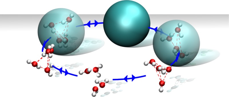
The adaptive resolution scheme (AdResS) is a multiscale molecular dynamics simulation approach that can concurrently couple atomistic (AT) and coarse-grained (CG) resolution regions, i.e., the molecules can freely adapt their resolution according to their current position in the system. Coupling to supramolecular CG models, where several molecules are represented as a single CG bead, is challenging, but it provides higher computational gains and connection to the established MARTINI CG force field. Difficulties that arise from such coupling have been so far bypassed with bundled AT water models, where additional harmonic bonds between oxygen atoms within a given supramolecular water bundle are introduced. While these models simplify the supramolecular coupling, they also cause in certain situations spurious artifacts, such as partial unfolding of biomolecules. In this work, we present a new clustering algorithm SWINGER that can concurrently make, break, and remake water bundles and in conjunction with the AdResS permits the use of original AT water models. We apply our approach to simulate a hybrid SPC/MARTINI water system and show that the essential properties of water are correctly reproduced with respect to the standard monoscale simulations. The developed hybrid water model can be used in biomolecular simulations, where a significant speed up can be obtained without compromising the accuracy of the AT water model.
1. Introduction
Contrary to the conventional monoscale molecular dynamics (MD) simulations, multiscale simulations1−16 can treat a given system simultaneously on different resolution scales, where each scale is described with a physically appropriate model for that particular scale. For example, in the context of biomolecular systems, the aqueous environment of macromolecules can be multiscaled, since a detailed (e.g., atomistic — AT) description is only required in the first hydration shell, whereas further away it is adequately treated on a simplified (e.g., coarse-grained — CG) level.17−20 As such, multiscale simulations can span larger spatiotemporal scales and thus provide computational and conceptual benefits.
Multiscale schemes where molecules can concurrently change their resolution, such as the adaptive resolution scheme (AdResS),21−26 require a mapping between high and low resolution representations. For AT/CG multiscale water, one strategy is a 1-to-1 mapping, where each water molecule is represented in the CG region as a single site, and the coordinates of a CG bead are set to match the center of mass (CoM) of the corresponding atoms.27 While such mapping is straightforward, the acquired speedup is rather limited. Per contra, N-to-1 mappings where multiple water molecules are merged to a single site in the CG region offer greater computational gains but bring about new challenges. Namely, the CoM correspondence between the AT and CG representations is no longer possible, since the CoM of several molecules becomes meaningless when they diffuse too far away from each other. In the particular case of water, the average lifetime of tetrahedral clusters due to hydrogen bonding is on a picosecond time scale.22
To circumvent this problem previous studies by our group28−30 and others31 have restricted the relative movement of water molecules that are mapped to the same CG bead and thus ensured that these molecules remained first neighbors during the total simulation run. The restriction can be achieved, as for example in the bundled-SPC models,32 via the introduction of attractive harmonic potentials between all oxygen pairs in a cluster. However, these restrictions can sometimes produce substantial side effects. For instance, a partial unfolding of the helices in a coiled-coil helix dimer33 can occur due to the bundled water. It is possible that the artifacts could be reduced if the restrictions were gradually weakened in the vicinity of the macromolecules thus enabling the clusters to deform and adopt to any local shape. Nevertheless, it is a matter of fact that the exact properties of the underlying AT model can only be reproduced in the limit of zero bundling.
An algorithm that would dynamically redistribute the water molecules into CG beads during the course of the simulation would therefore be very desirable as it would not require the use of the somewhat artificial bundled water models. In essence, the supramolecular mapping problem is similar to the one that the supramolecular structure-based coarse-graining techniques are facing. Algorithms for such purposes have been already developed; however, they are not applicable to multiscale simulations without substantial modifications. For example, the K-means34 algorithm, although very elegant, does not output clusters of a fixed number of molecules. In this respect, a more useful algorithm is the Monte Carlo (MC) based CUMULUS,35 but the algorithm leaves a small number of the molecules ungrouped. Moreover, both mentioned methods require a priori information about the number of clusters that will be formed.
In this paper, we present a novel methodology that facilitates supramolecular coupling in multiscale simulations. The SWINGER algorithm systematically assembles, disassembles, and reassembles clusters of multiple solvent molecules on-the-fly. The approach is employed to perform an AdResS simulation of a multiscale water system using a 4-to-1 mapping, where the standard AT SPC water model36 is coupled to the CG MARTINI37 water model.
2. Methods
2.1. Adaptive Resolution Scheme (AdResS)
The simulated system is split with respect to resolution along the x direction of the simulation box as schematically depicted in Figure 1. We depict only half of the (symmetric) simulation box, i.e., the box center is at the origin of the x-axis. The AT region is located at the center of the simulation box where water molecules are modeled with a three-site SPC36 model. As the water molecules move from the simulation box’s center to its edges they are first grouped to clusters each consisting of 4 water molecules. Then the resolution of clusters is smoothly changed from AT to CG via a transition hybrid (HY) region. In the CG region water is modeled with the MARTINI model.38,39 The latter is a popular biomolecular CG force field, which has been parametrized in a systematic way, based on the reproduction of partitioning free energies between polar and apolar phases of a large number of chemical compounds. The MARTINI force field uses a 4-to-1 mapping, i.e., on average four heavy atoms are represented by a single chargeless site. The number of degrees of freedom is thus significantly reduced, while still retaining chemical specificity required for biomolecular applications such as lipid self-assembly, peptide membrane binding, protein–protein recognition, etc.40
Figure 1.
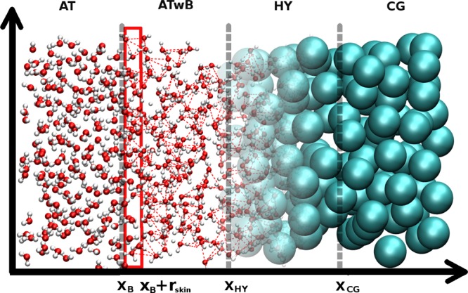
Schematic representation of half of the simulation box with atomistic (AT), atomistic with bundles (ATwB), hybrid (HY), and coarse-grained (CG) regions. Two levels of resolution are used for solvent molecules. High level of resolution is atomistic (SPC model), while the low level of resolution is supramolecular (MARTINI model). Boundaries between the regions are marked with dotted gray lines (xB = 7.2, xHY = 8.4, xCG = 9.6 nm), whereas the region C (X ∈ C; xB < X < xB + rskin, rskin = 0.2 nm), where the clusters are formed, is framed with red lines.
The coupling between different levels of resolution is carried out according to the AdResS scheme where the total force acting on a cluster α is
| 1 |
The Fαβat and Fαβ are the forces between clusters α and β, obtained from the AT and CG potentials, respectively. The sigmoidal function w ∈ [0,1] is used to smoothly couple the high and low resolution regimes, where Xα and Xβ are the distances in the x coordinate from the CoMs of clusters α and β to the center of the simulation box, respectively. The sigmoidal function w is equal to 1 in the AT + ATwB regions (x < xHY) and 0 in the CG region (x > xCG), and there is a smooth transition between the two values in the HY region, see Figure 1. The thermodynamic (TD) force FαTD is needed for the compensation of the difference in the chemical potential of AT and CG resolutions.41,42 In the AT region, where the clusters do not exist, the forces are purely atomistic as in the standard MD simulation.
Whenever we couple AT and CG models that have typically different chemical potentials (unless specifically parametrized to have matching potentials), as is the case with the MARTINI and bundled-SPC water model described below, or even if we couple two different models of the same resolution, having different chemical potentials, such as free SPC and bundled-SPC water models, density differences will occur across the simulation box. This is because the molecules with a higher chemical potential move into the region with a lower chemical potential. As just mentioned, to achieve a uniform density profile we have to compensate for the chemical potential differences between the respective AT and CG molecular models. This is accomplished by the external TD force FαTD, which is defined as a negative gradient of the excess chemical potential across the simulation box due to the intermolecular interactions.43 Skipping a few derivation steps that an interested reader can find in refs (41 and 42), the TD force computation translates into an iterative numerical formula
| 2 |
where C is an appropriately chosen numerical prefactor. This is similar to other methods for enforcing uniform density profile.44,45 The specific form of FαTD used in this study will be presented and explained in a bit more detail later on in section 3.
When the clusters (bundles) are formed (in cluster formation region C), an additional half-harmonic spring interaction is added between the oxygen atoms within a cluster. This interaction has the following form
 |
3 |
and
 |
4 |
where k = 1000 kJ mol–1 nm–2 is the force-constant, and rij and r0 = 0.3 nm are the current and equilibrium distance between oxygen atoms, respectively. The form and constants of the interaction are the same as in the bundled-SPC model 1.32 However, the oxygen–oxygen Lennard-Jones interaction is left here unaltered. In addition, the bundled interaction is multiplied with γ that depends on the CoM position X of the cluster. The function γ is used to obtain a smooth transition in a similar fashion as the w function is used in the AdResS scheme. Applying it, we avoid any large forces due to clustering and accommodate an easier reclustering. The region xB < x < xHY, where xB and xHY are transition boundaries between the standard SPC and bundled water and the AT and HY regions, respectively (see Figure 1), is still fully atomistic region and is thus named atomistic with bundles (ATwB) region. The minimal width of this region is set with the potential cutoff as in this region the CG interaction sites have to be defined to satisfy the AdResS scheme (see eq 1). Other MD simulation details are reported in the Supporting Information.
2.2. SWINGER: A Dynamic Clustering Algorithm
As already stated, the supramolecular coupling requires an algorithm that would dynamically make, break, and remake clusters. Specifically, the aim of the algorithm is to break clusters that have moved to the AT region and make or remake clusters in a predefined ”cluster formation” region C (see Figure 1) surrounding the AT region. The former part is straightforward, but the latter part entails an optimal grouping of data points, i.e., water molecules, into clusters, which is nontrivial. When developing our SWINGER algorithm we considered the following factors: (i) the number of molecules in a cluster has to be exactly 4 (due to the MARTINI model used as a CG model); (ii) preferentially, there should be no ungrouped molecules in the region C; (iii) the grouping should be optimized in terms of minimal total bundling energy ∑CUB of clusters in the region C; (iv) the algorithm should leave the coordinates and velocities of atoms intact.
Our clustering scheme SWINGER satisfies the mentioned requisites. The flowchart of SWINGER is depicted in Figure 2. At the first stage, all clusters whose CoMs are in the region C (X ∈ C; xB < X < xB+rskin) are disassembled. For the initial grouping two lists are constructed. The primary list contains molecules in region C, while the buffer list contains molecules with the X coordinate in the range xB – 2rskin < X < xB. The larger range of the buffer list is our conservative choice to make sure that the buffer list contains enough molecules at any given moment. Note that the lists contain both the molecules that were previously clustered and the ones that were not, but the algorithm does not distinguish the two cases.
Figure 2.
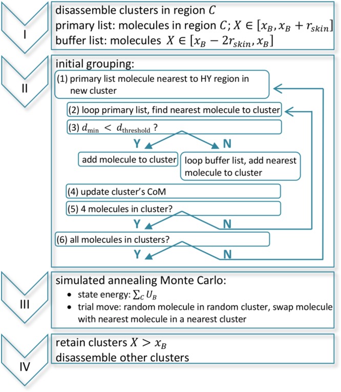
Flowchart of the SWINGER algorithm.
The procedure for the initial grouping is to (1) select the unassigned molecule in the primary list closest to the HY region and assign that molecule to a new cluster; (2) loop the unassigned molecules in the primary list and determine the cluster’s nearest molecule; (3) if the distance to the nearest molecule is less than the threshold value (0.4 nm in our case) add the molecule to the cluster, otherwise loop the unassigned molecules in the buffer list and add the nearest molecule; (4) update the cluster’s CoM; (5) repeat the steps (2–4) until the cluster contains 4 molecules; (6) repeat steps (1–5) until all molecules in the primary list are assigned to clusters.
Note that the number of water molecules considered for bundling is not predefined but an output of the initial grouping and depends on a given configuration. Additionally, initial grouping in an orderly fashion (the water molecules closest to the HY region are grouped first) outputs a grouping with a minimal number of water molecules from the buffer list and more optimized clusters closer to the HY region.
In the next stage, we employ the simulated annealing Monte Carlo (MC).46 The initial grouping outputs a clustering that serves as a good first guess. However, the clustering configuration is not optimal. The MC stage is used to refine the clustering and reach a global minimum configuration (defined as a minimum of ∑CUB, see below). As a result, we avoid possible large MD forces due to suboptimal clustering. Only one type of MC trial move is employed. We choose a random molecule in a random cluster. Then the nearest molecule belonging to a different cluster is determined, and the allocations of the two molecules are swapped. The energy of each state is ∑CUB, where UB is the bundling energy of an individual cluster defined in eq 3. However, instead of the γ function we use
| 5 |
This choice was made to avoid biased distribution of the clusters, i.e., if the γ function in eq 3 were used, the MC procedure would minimize the energy by outputting clusters whose CoM is shifted toward the AT region.
In the last stage, all clusters whose x coordinate of CoM is larger than xB are retained, while the others are disassembled. Because the cutoff is cluster-based some molecules in the region C might be left ungrouped. However, an important fact is that these molecules are facing the standard SPC AT region and are not located in between the clusters. The procedure of the SWINGER algorithm for a given configuration is depicted in Figure 3.
Figure 3.
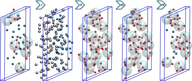
Algorithmic steps of the SWINGER algorithm. The snapshots represent the state of the system before and after each stage of the algorithm. Before the algorithm is applied the region C contains water molecules (blue) and water clusters (red). After the first stage (I) of the algorithm the clusters are disassembled, and primary (blue) and buffer (gray) lists are constructed. In the second stage (II), initial grouping is performed, where all molecules in the primary list are assigned to a given cluster. In the third stage (III), the clustering is optimized with simulated annealing MC. In the last stage (IV), only the clusters in region C are preserved, whereas other clusters are rejected.
Considering the typical lifetime of waters’ tetrahedral clusters, which is on the order of a ps,22 there is no need to perform the SWINGER at every MD step. However, it is necessary to execute it before unbundled water molecules are able to cross the xB + rskin boundary. We have decided to initiate the scheme at every Verlet list update, which constraints the minimal width of the region C to the size of the Verlet skin (we used rskin = 0.2 nm). The computational cost of the SWINGER algorithm depends on the size of the clustering region, i.e., on the number of water molecules M in the primary and adjacent buffer list. In particular, the algorithm’s complexity scales linearly with M as the energy of the simulated annealing MC involves only intracluster contributions. When the algorithm is employed the measured computational time of the MD time step is increased by approximately 5%. However, since the algorithm is, as mentioned before, not initiated at every time step, the overall increase in the computational load due to the SWINGER itself is negligible. However, the AdResS scheme does require an additional ATwB region, which is rcut = 1.2 nm wide. Hence, the simulation box enlargement due to the extra ATwB region represents the actual extra computational cost involved with coupling of the free SPC with the MARTINI water model. This depends on the simulation system under study. In our particular example, it corresponds to a computational cost of a bundled-SPC water MD simulation with a simulation box size of 2 × 1.2 × 2.8 × 2.8 nm3 (see the Supporting Information). Of course, with growing system size the relative computational overhead gets smaller.
To summarize, the AdResS scheme in combination with the SWINGER is able to couple the unmodified SPC AT water model with the MARTINI CG model. The results of such simulation are presented in the next section.
3. Results and Discussion
Due to inequality of the chemical potential at the AT and CG regions the molecules are prone to drifting toward the region with lower chemical potential, i.e., usually toward the CG region. We have introduced the TD force in the AdResS scheme that effectively corrects the unwanted density undulations. The TD force is iterated using the procedure, described in detail in refs (28, 41, and 42), until a uniform density profile is obtained. Since we have in our system two boundaries, where we couple different molecular models, the TD force is nonzero in the ATwB and HY regions. We could, in principle, consider two separate cases in computation of the TD force, i.e., a system with the free SPC and bundled-SPC waters and another system with the bundled-SPC and MARTINI waters and compute TD forces for each of them separately. Then we could glue the solutions to obtain the TD force for the merged system. Here, however, we have not followed this option. Rather, we have computed the TD force for the whole system in the same manner as in other AdResS simulations.28−30 The converged TD force is plotted in Figure 4. The force is, as customary, applied to the bundles’ CoM; however, here it acts not only in the HY region but also in the ATwB region. The extension of the force to the ATwB region is needed because the model is there effectively different than in the AT region due to the inclusion of the bundling potential. Indeed, the abrupt increase of the TD force at the onset of the ATwB region indicates the chemical potential difference between free SPC and bundled-SPC water models.32 If we changed the Lennard-Jones parameters of the oxygen atom in the ATwB region according to the bundled-SPC model, the extension would not be needed since the bundled-SPC model was parametrized to reproduce the same density, i.e., thermodynamic state. However, we did not do so as the current implementation avoids the possible spurious effects produced by the sudden change in the Lennard-Jones interaction when the molecule enters the ATwB region. It is also better suited for future applications of the multiscale model to solvate biomolecules where the biomolecule could interact also with the solvent molecules in the ATwB region.
Figure 4.
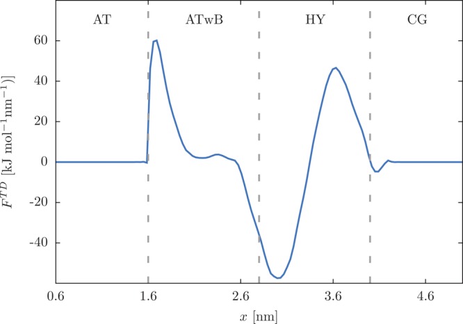
Thermodynamical (TD) force applied to the CoM of bundles. The force has a nonzero value only in the ATwB and HY regions. Vertical gray lines mark the resolution region boundaries.
With the TD force employed the obtained normalized density profiles (NDPs) are shown in Figure 5. The profiles are computed as a function of the x coordinate of the simulation box, i.e., along the direction of the resolution change. We plot separately the NDPs for the water oxygen atoms and bundles’ CoM and compare each of them with the appropriate reference all-atom simulation to point out that the variations in the density distribution are purely statistical in origin.
Figure 5.
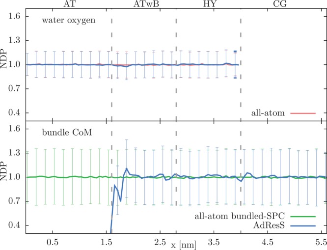
Normalized density profiles (NDPs) with standard deviations for water oxygen atoms (top) and bundles’ CoM (bottom). For normalization the bulk densities of oxygen atoms and water bundles are used in the top and bottom panels, respectively. Hence, the errors in the bottom figure are larger because of statistical reasons, i.e., there are 4 times more oxygen atoms than CG beads. The results are shown for the AdResS simulation and conventional all-atom simulations of SPC and bundled-SPC water (with changed Lennard-Jones parameters according to ref (32)) system. Vertical gray lines mark the resolution region boundaries.
Next, we check whether the AdResS methodology can preserve the local structure of the full-blown simulations. The radial distribution function (RDF), shown in Figure 6, is computed for the water oxygen atoms (top) and bundles’ COM (bottom). The AdResS RDFs are calculated only in the relevant regions, that is, the RDF computation of water oxygen atoms is restricted to molecules in the AT region and similarly the RDF of bundles’ CoM to those in the CG region. Comparison with the all-atom and coarse-grained simulations confirms a well reproduced local structure, with RDFs matching almost to the line thickness.
Figure 6.
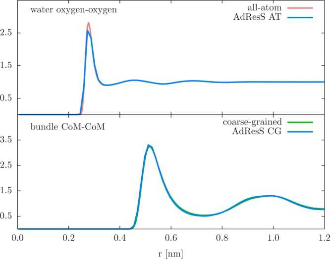
Radial distribution function (RDF) of oxygen atom (top) and bundle CoM or CG beads (bottom). The AdResS simulation results (AdResS AT and AdResS CG denote the region where the calculation is performed) are compared to the RDFs from reference all-atom and coarse-grained simulations to point out that the local structure is well reproduced.
Due to the hydrogen-bond network of water the short-range structure in water is roughly tetrahedral. The degree of this order can be measured with the tetrahedrality parameter Q4(47)
| 6 |
where the sum runs over distinct pairs of the four closest neighbors of the reference water molecule i, and θijk is the angle between vectors rij and rik with j and k being the nearest neighbors molecules. The summation is normalized to give the value of 0 for the random distribution. In Figure 7 we plot the tetrahedrality across different resolution regions. In the AT region the average value of Q4 is equal to the one found in the reference all-atom simulation. In the ATwB and HY regions the presence of half-harmonic bonds between oxygen atoms within bundles, as expected, distorts the local structure of water. We therefore observe a continuous decrease of the Q4 parameter as we move away from the AT region. Note that at the boundary between the ATwB and HY regions the average value of Q4 is equal to the average tetrahedrality of the bundled-SPC water model (with changed Lennard-Jones parameters according to ref (32)).
Figure 7.
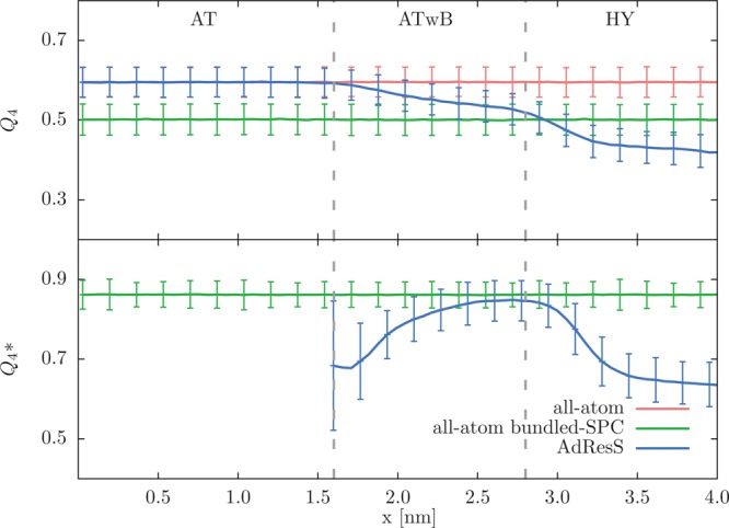
Tetrahedral order parameter Q4 (top) and Q4* (bottom) as a function of the x coordinate of the simulation box. The value of Q4 = 1 corresponds to a perfect tetrahedral arrangement, whereas Q4 = 0 describes an ideal gas. The error bars represent the standard deviation of the measurements. The results are shown for the AdResS, all-atom SPC, and all-atom bundled-SPC (with changed Lennard-Jones parameters according to ref (32)) simulations. The vertical dotted lines denote the boundaries between AT, ATwB, and HY regions.
The bundling promotes an internal structure of the bundles, where the water molecules are located at the 4 vertexes of the tetrahedron and the angle between two molecules and the bundle’s CoM is 109.5°. Internal ordering of the bundles can be described with the order parameter Q4* defined by
| 7 |
where i and j are the oxygen atoms of a distinct pair in a bundle, and ϕij is the angle between the two atoms and the bundle’s CoM. (Thus, the computation of Q4* involves four water molecules in a given bundle plus its CoM.) Thus, as the strength of the bundling is increased in the ATwB region the promoted order also increases and reaches the value Q4 found in the bundled-SPC water model. In the HY region both order parameters decline as a result of the resolution change.
Next, we compute the average bundling energy UB profile (Figure 8) by discretizing x positions in the system into bins and taking the average over bundles that fall into a corresponding bin. The energies in the cluster formation region are quite high even though the clustering is optimized because the Q4* internal structure is not inherent to the standard SPC water. This is why it is better to introduce bundling in a smooth way via the γ function (full line) and thus avoid any large forces. By the time the bundles enter the HY region they are well equilibrated with energies of comparable magnitude that are found in the bundled-SPC system.
Figure 8.
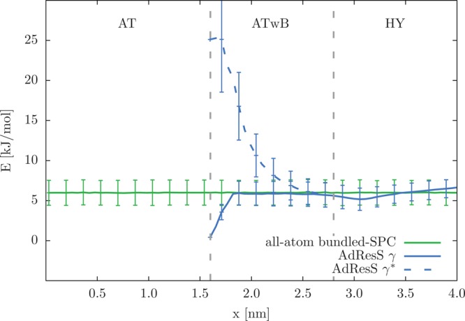
Average bundling energy of a bundle (UB; eq 3) with standard deviations along the direction of the resolution change. The results are plotted for the AdResS simulation and reference all-atom simulation of bundled-SPC water (with changed Lennard-Jones parameters according to ref (32)). The AdResS profile is computed separately for the γ and γ* functions (eqs 4 and 5, respectively). Resolution region boundaries are denoted with the vertical gray lines.
From the dynamics perspective, an important property of our SWINGER algorithm and multiscale approach is the free movement of the molecules across all regions. In Figure 9 we show the time evolution of the concentration profiles of water oxygen atoms. The molecules are initially in the ATwB or HY regions but diffuse in time throughout the whole simulation box. Molecules spread out unequally to the AT and HY regions which is in accordance with different diffusion coefficients of the SPC and bundled-SPC water models.28,32 The estimated diffusion constants, which are extracted by fitting the Green’s function for the diffusion equation to the concentration profiles, are 5.1 × 10⁻⁹ m2 s–1 and 2.1 × 10⁻⁹ m2 s–1 (error bars are roughly 10%) for free SPC and bundled-SPC, respectively. The diffusion of the bundled-SPC water is slower than that of free SPC water due to the larger hydrodynamic radius of the bundles compared to the single SPC molecules. This is in agreement with previously published simulation results.28 Interestingly, the diffusion constant of the bundled-SPC is closer to the experimental value of 2.4 × 10⁻⁹ m2 s–1.48
Figure 9.
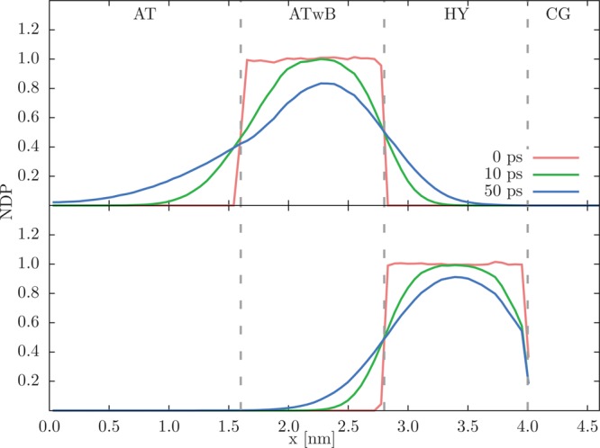
Diffusion of oxygen atoms across different resolution regions. Top: Normalized density distributions of particles at time t = 0 ps (red) in the ATwB region and at times t = 10 ps (green) and t = 50 ps (blue). Bottom: The same time evolution for particles initially in the HY region. The concentration profiles are not depicted in the CG region because the profiles are computed for oxygen atoms and the AT resolution is absent in the CG region. Vertical gray lines denote the boundaries between different regions.
Rotational dynamics is characterized by rotational relaxation time and associated single water molecule dipole autocorrelation function49
| 8 |
where n is a unit vector pointing along the dipole moment of a water molecule. The autocorrelation function dACF(t) is depicted in Figure 10 for the free SPC water model from the all-atom simulation and the AT region of the AdResS simulation. The extracted rotational relaxation time τ is 3.3 ps ± 0.2 ps for water molecules from the reference all-atom simulation and AT region of the AdResS simulation. This is in good agreement with the simulation results in the literature49 but lower than the experimental value of 7.5 ps.51 We ascribe this discrepancy to the SPC water model and not to our multiscale approach.
Figure 10.
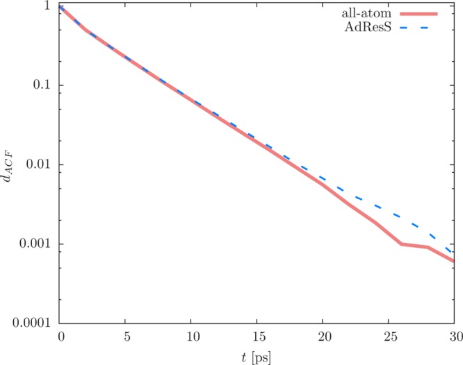
Dipole autocorrelation function dACF(t) as defined by eq 8. We average over water molecules that are initially in the AT region.50
The concentration profiles, dipole autocorrelation functions, and the corresponding diffusion constants and rotational relaxation times thus prove that the SWINGER algorithm does in fact make, break, and remake clusters and does so without disturbing the dynamics of the system.
4. Conclusions
In conclusion, we have demonstrated how to successfully overcome the challenge of carrying out multiscale simulations with supramolecular mapping. The presented SWINGER algorithm is a dynamic mapping scheme; i.e., it assembles, disassembles, and reassembles clusters as needed during the course of the simulation. With little computational overhead cost we can, therefore, use the standard AT water models in the region of interest and thereby avoid spurious side effects.33
Our methodology was tested on a SPC/MARTINI water model system, but it is easily transferable to other AT models, such as SPC/E,52 TIP3P,53 TIP4P,53 etc. and other CG models, e.g., the polarizable MARTINI water model.54 With minimal modifications it could also be applied to other mappings, for example, 5-to-1 and used in connection with the model of Riniker et al.55 Moreover, the SWINGER algorithm could be also employed in other multiscale schemes, e.g., H-AdResS.15,16 In all cases the multiscale simulations of such systems can (in the AT region) fully reproduce the statistical properties of the conventional atomistic simulations. The presented multiscale approach thus allows for a seamless coupling between standard atomistic and supramolecular water models and paves the way for efficient MD simulations of biomolecular systems. In a future perspective, we envision that SWINGER in combination with AdResS could be also employed for coupling atomistic water with even more simplified CG models bridging to the hydrodynamics scale as for example in coupling of MD with multiparticle collision dynamics56 or coupling MD with continuum hydrodynamics, such as in ref (57). There one should resort to other means58 to keep the water molecules together instead of semiharmonic bonds. Another interesting application could be using SWINGER to postprocess an all-atom MD simulation to derive new CG model parameters exploiting, for example, structure-based coarse-graining techniques.
Acknowledgments
J.Z. and M.P. acknowledge financial support through the grants P1-0002 and J1-7435 from the Slovenian Research Agency. S.J.M. acknowledges support from the ERC Advanced grant 669723 - COMP-MICR-CROW-MEM.
Supporting Information Available
The Supporting Information is available free of charge on the ACS Publications website at DOI: 10.1021/acs.jctc.6b00536.
Additional results and simulation details (PDF)
The authors declare no competing financial interest.
Supplementary Material
References
- Gonzalez O.; Petkeviciute D.; Maddocks J. H. J. Chem. Phys. 2013, 138, 055102. 10.1063/1.4789411. [DOI] [PubMed] [Google Scholar]
- Ensing B.; Nielsen S. O.; Moore P. B.; Klein M. L.; Parrinello M. J. Chem. Theory Comput. 2007, 3, 1100. 10.1021/ct600323n. [DOI] [PubMed] [Google Scholar]
- Szklarczyk O. M.; Bieler N. S.; Hünenberger P. H.; van Gunsteren W. F. J. Chem. Theory Comput. 2015, 11, 5447–5463. 10.1021/acs.jctc.5b00406. [DOI] [PubMed] [Google Scholar]
- Michel J.; Orsi M.; Essex J. W. J. Phys. Chem. B 2008, 112, 657–660. 10.1021/jp076142y. [DOI] [PubMed] [Google Scholar]
- Masella M.; Borgis D.; Cuniasse P. J. Comput. Chem. 2011, 32, 2664–2678. 10.1002/jcc.21846. [DOI] [PubMed] [Google Scholar]
- Goga N.; Melo M. N.; Rzepiela A. J.; de Vries A. H.; Hadar A.; Marrink S. J.; Berendsen H. J. C. J. Chem. Theory Comput. 2015, 11, 1389–1398. 10.1021/ct501102b. [DOI] [PubMed] [Google Scholar]
- Machado M. R.; Dans P. D.; Pantano S. Phys. Chem. Chem. Phys. 2011, 13, 18134–18144. 10.1039/c1cp21248f. [DOI] [PubMed] [Google Scholar]
- Yan X. C.; Tirado-Rives J.; Jorgensen W. L. J. Phys. Chem. B 2016, 10.1021/acs.jpcb.6b00399. [DOI] [PMC free article] [PubMed] [Google Scholar]
- Sokkar P.; Boulanger E.; Thiel W.; Sanchez-Garcia E. J. Chem. Theory Comput. 2015, 11, 1809–1818. 10.1021/ct500956u. [DOI] [PubMed] [Google Scholar]
- Shi Q.; Izvekov S.; Voth G. A. J. Phys. Chem. B 2006, 110, 15045–15048. 10.1021/jp062700h. [DOI] [PubMed] [Google Scholar]
- Petsev N. D.; Leal L. G.; Shell M. S. J. Chem. Phys. 2016, 144, 084115. 10.1063/1.4942499. [DOI] [PMC free article] [PubMed] [Google Scholar]
- Walther J. H.; Praprotnik M.; Kotsalis E. M.; Koumoutsakos P. J. Comput. Phys. 2012, 231, 2677–2681. 10.1016/j.jcp.2011.12.015. [DOI] [Google Scholar]
- Alekseeva U.; Winkler R. G.; Sutmann G. J. Comput. Phys. 2016, 314, 14–34. 10.1016/j.jcp.2016.02.065. [DOI] [Google Scholar]
- Abrams C. F. J. Chem. Phys. 2005, 123, 234101. 10.1063/1.2136884. [DOI] [PubMed] [Google Scholar]
- Potestio R.; Fritsch S.; Español P.; Delgado-Buscalioni R.; Kremer K.; Everaers R.; Donadio D. Phys. Rev. Lett. 2013, 110, 108301. 10.1103/PhysRevLett.110.108301. [DOI] [PubMed] [Google Scholar]
- Potestio R.; Español P.; Delgado-Buscalioni R.; Everaers R.; Kremer K.; Donadio D. Phys. Rev. Lett. 2013, 111, 060601. 10.1103/PhysRevLett.111.060601. [DOI] [PubMed] [Google Scholar]
- Hijón C.; Español P.; Vanden-Eijnden E.; Delgado-Buscalioni R. Faraday Discuss. 2010, 144, 301–322. 10.1039/B902479B. [DOI] [PubMed] [Google Scholar]
- Li Z.; Bian X.; Caswell B.; Karniadakis G. E. Soft Matter 2014, 10, 8659–8672. 10.1039/C4SM01387E. [DOI] [PubMed] [Google Scholar]
- Harmandaris V.; Kalligiannaki E.; Katsoulakis M.; Plecháč P. J. Comput. Phys. 2016, 314, 355–383. 10.1016/j.jcp.2016.03.021. [DOI] [Google Scholar]
- Dannenhoffer-Lafage T.; White A. D.; Voth G. A. J. Chem. Theory Comput. 2016, 12, 2144–2153. 10.1021/acs.jctc.6b00043. [DOI] [PubMed] [Google Scholar]
- Praprotnik M.; Delle Site L.; Kremer K. J. Chem. Phys. 2005, 123, 224106. 10.1063/1.2132286. [DOI] [PubMed] [Google Scholar]
- Praprotnik M.; Delle Site L.; Kremer K. Annu. Rev. Phys. Chem. 2008, 59, 545–571. 10.1146/annurev.physchem.59.032607.093707. [DOI] [PubMed] [Google Scholar]
- Wang H.; Hartmann C.; Schütte C.; Delle Site L. Phys. Rev. X 2013, 3, 011018. 10.1103/PhysRevX.3.011018. [DOI] [Google Scholar]
- Agarwal A.; Delle Site L. J. Chem. Phys. 2015, 143, 094102. 10.1063/1.4929738. [DOI] [PubMed] [Google Scholar]
- Wang H.; Agarwal A. Eur. Phys. J.: Spec. Top. 2015, 224, 2269–2287. 10.1140/epjst/e2015-02411-2. [DOI] [Google Scholar]
- Kreis K.; Fogarty A.; Kremer K.; Potestio R. Eur. Phys. J.: Spec. Top. 2015, 224, 2289–2304. 10.1140/epjst/e2015-02412-1. [DOI] [Google Scholar]
- Praprotnik M.; Matysiak S.; Delle Site L.; Kremer K.; Clementi C. J. Phys.: Condens. Matter 2007, 19, 292201. 10.1088/0953-8984/19/29/292201. [DOI] [Google Scholar]
- Zavadlav J.; Melo M. N.; Cunha A. V.; de Vries A. H.; Marrink S. J.; Praprotnik M. J. Chem. Theory Comput. 2014, 10, 2591–2598. 10.1021/ct5001523. [DOI] [PubMed] [Google Scholar]
- Zavadlav J.; Melo M. N.; Marrink S. J.; Praprotnik M. J. Chem. Phys. 2014, 140, 054114. 10.1063/1.4863329. [DOI] [PubMed] [Google Scholar]
- Zavadlav J.; Melo M. N.; Marrink S. J.; Praprotnik M. J. Chem. Phys. 2015, 142, 244118. 10.1063/1.4923008. [DOI] [PubMed] [Google Scholar]
- Nagarajan A.; Junghans C.; Matysiak S. J. Chem. Theory Comput. 2013, 9, 5168–5175. 10.1021/ct400566j. [DOI] [PubMed] [Google Scholar]
- Fuhrmans M.; Sanders B. P.; Marrink S. J.; de Vries A. H. Theor. Chem. Acc. 2010, 125, 335–344. 10.1007/s00214-009-0590-4. [DOI] [Google Scholar]
- Gopal S. M.; Kuhn A. B.; Schäfer L. V. Phys. Chem. Chem. Phys. 2015, 17, 8393–8406. 10.1039/C4CP04784B. [DOI] [PubMed] [Google Scholar]
- Hadley K. R.; McCabe C. J. Phys. Chem. B 2010, 114, 4590–4599. 10.1021/jp911894a. [DOI] [PMC free article] [PubMed] [Google Scholar]
- van Hoof B.; Markvoort A. J.; van Santen R. A.; Hilbers P. A. J. J. Phys. Chem. B 2011, 115, 10001–10012. 10.1021/jp201975m. [DOI] [PubMed] [Google Scholar]
- Berendsen H. J. C.; Postma J. P. M.; van Gunsteren W. F.; Hermans J. Intermolecular Forces 1981, 14, 331–342. 10.1007/978-94-015-7658-1_21. [DOI] [Google Scholar]
- Marrink S. J.; de Vries A. H.; Mark A. E. J. Phys. Chem. B 2004, 108, 750–760. 10.1021/jp036508g. [DOI] [Google Scholar]
- Marrink S. J.; Risselada H. J.; Yefimov S.; Tieleman D. P.; de Vries A. H. J. Phys. Chem. B 2007, 111, 7812–7824. 10.1021/jp071097f. [DOI] [PubMed] [Google Scholar]
- Monticelli L.; Kandasamy S. K.; Periole X.; Larson R. G.; Tieleman D. P.; Marrink S. J. J. Chem. Theory Comput. 2008, 4, 819–834. 10.1021/ct700324x. [DOI] [PubMed] [Google Scholar]
- Marrink S. J.; Tieleman D. P. Chem. Soc. Rev. 2013, 42, 6801–6822. 10.1039/c3cs60093a. [DOI] [PubMed] [Google Scholar]
- Praprotnik M.; Poblete S.; Kremer K. J. Stat. Phys. 2011, 145, 946–966. 10.1007/s10955-011-0312-x. [DOI] [Google Scholar]
- Fritsch S.; Poblete S.; Junghans C.; Ciccotti G.; Delle Site L.; Kremer K. Phys. Rev. Lett. 2012, 108, 170602. 10.1103/PhysRevLett.108.170602. [DOI] [PubMed] [Google Scholar]
- Poblete S.; Praprotnik M.; Kremer K.; Delle Site L. J. Chem. Phys. 2010, 132, 114101. 10.1063/1.3357982. [DOI] [PubMed] [Google Scholar]
- Kotsalis E. M.; Walther J. H.; Koumoutsakos P. Phys. Rev. E 2007, 76, 016709. 10.1103/PhysRevE.76.016709. [DOI] [PubMed] [Google Scholar]
- Kotsalis E. M.; Walther J. H.; Kaxiras E.; Koumoutsakos P. Phys. Rev. E 2009, 79, 045701. 10.1103/PhysRevE.79.045701. [DOI] [PubMed] [Google Scholar]
- Kirkpatrick S.; Gelatt C. D. Jr.; Vecchi M. P. Science 1983, 220, 671–680. 10.1126/science.220.4598.671. [DOI] [PubMed] [Google Scholar]
- Errington J. R.; Debenedetti P. G. Nature 2001, 409, 318–321. 10.1038/35053024. [DOI] [PubMed] [Google Scholar]
- Prevost M.; van Belle D.; Lippens G.; Wodak S. Mol. Phys. 1990, 71, 587–603. 10.1080/00268979000101991. [DOI] [Google Scholar]
- Praprotnik M.; Janežič D. J. Chem. Phys. 2005, 122, 174103. 10.1063/1.1884609. [DOI] [PubMed] [Google Scholar]
- Delle Site L. Phys. Rev. E: Stat. Phys., Plasmas, Fluids, Relat. Interdiscip. Top. 2016, 93, 022130. 10.1103/PhysRevE.93.022130. [DOI] [Google Scholar]
- Wallqvist A.; Berne B. J. J. Phys. Chem. 1993, 97, 13841–13851. 10.1021/j100153a066. [DOI] [Google Scholar]
- Berendsen H. J. C.; Grigera J. R.; Straatsma T. P. J. Phys. Chem. 1987, 91, 6269–6271. 10.1021/j100308a038. [DOI] [Google Scholar]
- Jorgensen W. L.; Chandrasekhar J.; Madura J. D.; Impey R. W.; Klein M. L. J. Chem. Phys. 1983, 79, 926–935. 10.1063/1.445869. [DOI] [Google Scholar]
- Yesylevskyy S. O.; Schäfer L. V.; Sengupta D.; Marrink S. J. PLoS Comput. Biol. 2010, 6, e1000810. 10.1371/journal.pcbi.1000810. [DOI] [PMC free article] [PubMed] [Google Scholar]
- Riniker S.; van Gunsteren W. F. J. Chem. Phys. 2011, 134, 084110. 10.1063/1.3553378. [DOI] [PubMed] [Google Scholar]
- Alekseeva U.; Winkler R. G.; Sutmann G. J. Comput. Phys. 2016, 314, 14–34. 10.1016/j.jcp.2016.02.065. [DOI] [Google Scholar]
- Scukins A.; Nerukh D.; Pavlov E.; Karabasov S.; Markesteijn A. Eur. Phys. J.: Spec. Top. 2015, 224, 2217–2238. 10.1140/epjst/e2015-02409-8. [DOI] [Google Scholar]
- Usabiaga F.; Bell J.; Delgado-Buscalioni R.; Donev A.; Fai T.; Griffith B.; Peskin C. Multiscale Model. Simul. 2012, 10, 1369–1408. 10.1137/120864520. [DOI] [Google Scholar]
Associated Data
This section collects any data citations, data availability statements, or supplementary materials included in this article.


