

Abstract
Background:
Ambient monitoring data show spatial gradients in ozone (O3) across urban areas. Nitrogen oxide (NOx) emissions reductions will likely alter these gradients. Epidemiological studies often use exposure surrogates that may not fully account for the impacts of spatially and temporally changing concentrations on population exposure.
Objectives:
We examined the impact of large NOx decreases on spatial and temporal O3 patterns and the implications on exposure.
Methods:
We used a photochemical model to estimate O3 response to large NOx reductions. We derived time series of 2006–2008 O3 concentrations consistent with 50% and 75% NOx emissions reduction scenarios in three urban areas (Atlanta, Philadelphia, and Chicago) at each monitor location and spatially interpolated O3 to census-tract centroids.
Results:
We predicted that low O3 concentrations would increase and high O3 concentrations would decrease in response to NOx reductions within an urban area. O3 increases occurred across larger areas for the seasonal mean metric than for the regulatory metric (annual 4th highest daily 8-hr maximum) and were located only in urban core areas. O3 always decreased outside the urban core (e.g., at locations of maximum local ozone concentration) for both metrics and decreased within the urban core in some instances. NOx reductions led to more uniform spatial gradients and diurnal and seasonal patterns and caused seasonal peaks in midrange O3 concentrations to shift from midsummer to earlier in the year.
Conclusions:
These changes have implications for how O3 exposure may change in response to NOx reductions and are informative for the design of future epidemiology studies and risk assessments.
Citation:
Simon H, Wells B, Baker KR, Hubbell B. 2016. Assessing temporal and spatial patterns of observed and predicted ozone in multiple urban areas. Environ Health Perspect 124:1443–1452; http://dx.doi.org/10.1289/EHP190
Introduction
Exposure to ozone (O3) is known to cause negative health effects in humans [U.S. Environmental Protection Agency (EPA) 2013]. Many areas in the United States currently experience O3 concentrations that exceed the National Ambient Air Quality Standards (NAAQS) (https://ozoneairqualitystandards.epa.gov/OAR_OAQPS/OzoneSliderApp/index.html#). Although there have been substantial emission reductions of O3 precursors, and peak O3 concentrations have decreased as a result of these reductions, some areas are expected to continue to exceed the 8-hr O3 NAAQS in the future (U.S. EPA 2014b).
Nitrogen oxide (NOx) and volatile organic compound (VOC) emissions react in the atmosphere through complex nonlinear chemical reactions to form ground-level O3 when meteorological conditions are favorable (Seinfeld and Pandis 2012). Specifically, NOx participates in chemical pathways for both O3 formation and destruction; therefore, the net impact of NOx emissions on O3 concentrations depends on the relative abundances of NOx, VOCs, and sunlight as well as on the temporal and spatial scales being examined. Emissions sources of NOx and VOC and the resulting O3 vary seasonally, diurnally, and spatially. Spatial differences exist from rural to urban, city to city, and even within a given urban area (Marshall et al. 2008). In locations with high concentrations of nitric oxide (NO), one component of NOx, O3 can become artificially suppressed owing to direct reactions of NO with O3. These reactions also result in the production of other oxidized nitrogen species, which form O3 away from the emission source location while the wind transports the air mass, thus contributing to elevated O3 downwind (Cleveland and Graedel 1979). As a result of this chemistry, decreasing NOx and VOC emissions generally decrease O3 at times and locations in which O3 concentrations are high (Simon et al. 2013). In limited circumstances, reductions of NOx emissions can lead to O3 increases in the immediate vicinity of highly concentrated NOx sources, whereas these same emissions changes generally lead to reductions of O3 downwind over longer timescales (Cleveland and Graedel 1979; Kelly et al. 2015; Murphy et al. 2007; Sillman 1999; Xiao et al. 2010). Because emissions of both NOx and VOC decrease from sources that have unique temporal and spatial attributes (e.g., power plant NOx and mobile source NOx and VOCs), it will be important to characterize how O3 formation regimes vary over different temporal and spatial scales in order to understand how O3 concentrations may change as a result of these emissions reductions.
Spatial and temporal variability in pollutant concentrations are key inputs to studies evaluating associations between air quality and human health. In the past, epidemiological studies linking O3 with human health impacts have used ambient measurements in various ways to match against health outcomes. Some studies have used spatially averaged O3 concentrations for an entire urban area to link with short-term (Smith et al. 2009; Zanobetti and Schwartz 2008) and long-term (Jerrett et al. 2009) mortality. Other studies have used the O3 monitor closest to the residence of the human subjects (Bell 2006). The use of an average “composite” monitor masks both spatial and temporal heterogeneity that exist in an urban area. Using the nearest monitor may provide a better spatial match but does not fully consider daily activity patterns. Given the spatial and temporal heterogeneity in O3 and human activity patterns that place a subject in different places at different times of the day, it is potentially important to match activity with a realistic heterogeneous representation of O3 concentrations. This is true for conducting epidemiology studies of O3 health outcomes, as well as in the application of the results of those studies in risk and health impact assessments. To the extent that reductions in NOx and VOC emissions change the temporal and spatial patterns of O3, the use of a spatially averaged O3 concentration may mask how population-weighted O3 exposures change.
Recent risk assessments conducted to inform the U.S. EPA review of the O3 NAAQS included application of results from both controlled human exposure studies and observational epidemiology studies (U.S. EPA 2014a). Estimates of risk based on controlled human exposure studies evaluated changes in the risk of 10% and 15% lung function decrements and used an exposure–response model that was more responsive to changes in exposure when the maximum daily 8-hr average (MDA8) O3 was > 40 ppb. In contrast, estimates of risk based on the application of results from epidemiology studies used linear, no-threshold concentration–response functions, so an incremental change in O3 affected total risk equally, regardless of the starting level of O3. As a result, the epidemiology-based risk estimates could be quite sensitive to the patterns of O3 responses to NOx reductions, whereas the risk estimates based on controlled human exposure studies reflected the changes that occurred at the higher O3 concentrations.
Given the complex nature of O3 chemistry and emissions source mixes in a given urban area, photochemical grid models provide a credible tool for evaluating responsiveness to emissions changes and have been used extensively for O3 planning purposes in the past (Cai et al. 2011; Hogrefe et al. 2011; Kumar and Russell 1996; Simon et al. 2012). In the present study, we used a photochemical grid model applied in three different urban areas to illustrate temporal and spatial patterns of O3 and how those patterns may change as a result of reduced precursor emissions. Model-predicted changes in O3 were aggregated using several metrics to show how spatial heterogeneity depends on the O3 metric that is being analyzed and how the type of aggregation used can mute the spatial variability in O3 response to emissions changes.
Methods
City Selection And Monitoring Data
Three major urban areas (Philadelphia, Atlanta, and Chicago) were selected for evaluation based on the spatial coverage of the local ambient monitoring network and because they demonstrate different types of spatial O3 patterns and responses to emissions changes (U.S. EPA 2014a). In addition, the photochemical model performed well in these cities (U.S. EPA 2014a). For each urban area, all ambient monitoring sites within the combined statistical area (CSA) were included in the analysis as well as any additional monitoring sites within a 50-km buffer of the CSA boundary. Hourly average O3 data from these ambient monitoring sites for the years 2006–2008 were obtained from the U.S. EPA’s Air Quality System (AQS) database (http://www2.epa.gov/aqs).
Ambient Data Adjustments to Estimate O3 Distributions under Alternate Emissions
We applied outputs from a series of photochemical air quality model simulations to estimate how hourly O3 could change under hypothetical scenarios of 50% and 75% reductions in U.S. anthropogenic NOx emissions. Emissions projections from the U.S. EPA predict substantial reductions (45%) in U.S. anthropogenic NOx between 2007 and 2020 (U.S. EPA 2012). VOC emissions are also expected to decline between 2007 and 2020 by a more modest 20% (U.S. EPA 2012). By evaluating O3 concentrations at 50% and 75% NOx reductions, we were able to look at O3 responses for two scenarios of varying emissions. Although the primary focus of this study was on NOx reduction scenarios, we also included a more limited evaluation of scenarios where both NOx and VOC emissions were reduced by 50% and 75% to determine how cooccurring VOC reductions could change patterns of responses to NOx reductions.
The methodology for adjusting observed O3 to scenarios of 50% and 75% NOx reductions was adapted from the methods developed by Simon et al. (2013) and by the U.S. EPA (2014a). However, both of these studies targeted specific air quality goals rather than emissions reduction levels as were investigated here. The methods are described in detail in those documents and are summarized below.
We used the Community Multi-scale Air Quality (CMAQ) model v.4.7.1 instrumented with higher-order decoupled direct method (HDDM) capabilities to calculate O3 responses to emissions inputs. Details on the model setup and inputs are provided in the Supplemental Material (“Supplemental Methods”). Model predictions of MDA8 O3 were compared with monitored values in each of the three cities. Overall, the mean biases were 3.7 ppb, 2 ppb, and 1 ppb in Atlanta, Chicago, and Philadelphia, respectively. The Pearson correlations (R) were 0.82, 0.86, and 0.88, respectively. A seasonal breakout of these performance statistics is provided in Table S1. This model performance is within the range of what has been observed in state-of-the-science ozone modeling reported in recent studies (Simon et al. 2012) and is sufficiently accurate for the purpose of this analysis.
The CMAQ-HDDM system provided outputs of hourly O3 and hourly sensitivity coefficients at a 12 km × 12 km grid resolution across the contiguous United States. These sensitivities describe a nonlinear (quadratic) O3 response at a specified time and location to an across-the-board perturbation in NOx emissions following Equation 1:
 |
[1] |
where ΔO3h,l is the change in O3 at hour h and location l, Δε is the relative change in NOx emissions (e.g., –0.2 represents a 20% reduction in NOx emissions) and S 1 h,l and S 2 h,l represent the first- and second-order O3 sensitivity coefficients at hour h and location l.
Model simulations were performed for 7 months in 2007 (January and April–October), which provided O3 responses over a range of emissions and meteorological conditions and provided information on seasonal variations in the response. To apply the modeled sensitivity coefficients from 7 months to 3 years of ambient measurements (described above), we derived statistical relationships between the modeled sensitivity coefficients and the modeled hourly O3 concentrations using linear regression. Separate linear regressions were created for each monitor location at each hour of the day and for each season, resulting in a total of 96 (24 hr × 4 seasons) linear regressions for the first- and second-order sensitivity coefficients at each monitor location. The linear regression resulted in statistically significant relationships between ozone concentration and responsiveness to NOx emissions reductions for most combinations of hours of the day, season, and monitoring location. Using these relationships, we could determine the first- and second-order sensitivity coefficients at O3 monitor locations for every hour of 2006–2008. Finally, we used Equation 1 to predict the change in measured ambient O3 concentrations for a set change in NOx emissions at each monitor location.
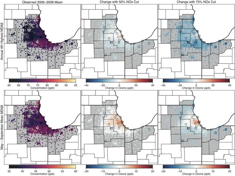
Figure 2.

Maps showing the 2006–2008 average annual 4th-highest maximum daily 8-hr average ozone (MDA8 O3), the regulatory metric, (parts per billion; top panels) and May–September mean MDA8 O3 (parts per billion; bottom panels) values in Philadelphia for observed conditions (left panels), and predicted changes with 50% U.S. nitrogen oxide (NOx) emissions reductions (center panels) and 75% U.S. NOx emissions reductions (right panels). Colored squares show locations of monitoring sites, and colored dots show interpolated values at census-tract centroids.
An additional complication is introduced when looking at large changes in NOx emissions (e.g., 50% and 75%). Previous studies have reported that CMAQ-HDDM estimates of O3 changes are most accurate for emissions perturbations < 50% (Hakami et al. 2003). To address this issue, we ran the CMAQ-HDDM model at two distinct emissions levels (2007 emissions and 50% NOx conditions) to derive emissions sensitivity coefficients that would occur under different emissions regimes. We then developed a two-step adjustment methodology in which sensitivity coefficients from each of the simulations were applied over the portion of emissions reductions for which they were most applicable (Simon et al. 2013; U.S. EPA 2014a). The exact point over the emissions reduction glide-path at which the sensitivity was switched differed for each city and was determined by minimizing the least square error between the adjusted O3 concentrations using the two-step approach and actual modeled concentrations from “brute force” NOx cut simulations. Analyses presented by the U.S. EPA (2014a) showed that this two-step approach could replicate O3 changes for 50% emissions reductions with mean bias between –0.2 and –0.9 ppb and mean absolute error equal to 1 ppb for the three cities evaluated here.
Spatial Interpolation
To better examine spatial patterns in O3 concentrations and population exposure, we used the Voronoi neighbor averaging (VNA) (Gold et al. 1997; Chen et al. 2004) method to create spatial fields of the hourly O3 in each urban area for the observed, 50% NOx cut, and 75% NOx cut scenarios. We used VNA to interpolate the observed or adjusted hourly concentration data using an inverse distance squared weighting from monitored locations to each census tract centroid within the CSA boundaries of each urban area. The resulting spatial fields provided temporally complete estimates of observed and adjusted hourly O3 concentrations at refined spatial resolution within each urban area. Previous cross-validation tests showed that this interpolation method provided good performance at urban scales (U.S. EPA 2014a).
Results
Predicted Spatial Changes
We focused on two MDA8 O3 metrics for our assessment: the annual 4th-highest MDA8 value averaged over 3 consecutive years, which corresponds to the form and averaging time of the current O3 NAAQS and represents O3 concentrations on the highest O3 days (also known as the “design value” and hereafter referred to as the regulatory metric), and the May–September mean of the MDA8 (i.e., the seasonal mean metric), which generally tracks well with estimates of epidemiology-based O3 health risk (U.S. EPA 2014a). Maps of VNA surfaces showing spatial patterns in these metrics for Atlanta, Philadelphia, and Chicago are presented in Figures 1–3. The left panels show the values based on measured O3 concentrations, and the center and right panels show the changes in these observed values under the 50% and 75% NOx cut scenarios, respectively.
Figure 1.

Maps showing the 2006–2008 average annual 4th-highest maximum daily 8-hr average ozone (MDA8 O3), the regulatory metric (parts per billion; top panels), and May–September mean MDA8 O3 (parts per billion; bottom panels) values in Atlanta for observed conditions (left panels), and predicted changes with 50% U.S. nitrogen oxide (NOx) emissions reductions (center panels) and 75% U.S. NOx emissions reductions (right panels). Colored squares show locations of monitoring sites, and colored dots show interpolated values at census-tract centroids.
Figure 3.
Maps showing the 2006–2008 average annual 4th-highest maximum daily 8-hr average ozone (MDA8 O3), the regulatory metric, (parts per billion; top panels) and May–September mean MDA8 O3 (parts per billion; bottom panels) values in Chicago for observed conditions (left panels), and predicted changes with 50% U.S. nitrogen oxide (NOx) emissions reductions (center panels) and 75% U.S. NOx emissions reductions (right panels). Colored squares show locations of monitoring sites, and colored dots show interpolated values at census-tract centroids.
For the observed scenario, Atlanta had fairly uniform O3 concentrations (particularly for the seasonal average), whereas Philadelphia and Chicago had sharp spatial gradients owing to local O3 suppression near NO emissions sources in the urban core and subsequent O3 formation downwind as described in the introduction. When considering the predicted changes in the two metrics under the 50% and 75% NOx cut scenarios, each city displayed a different spatial pattern. In Atlanta, large NOx reductions were predicted to result in fairly uniform decreases in both O3 metrics across the CSA, although the decreases were slightly less pronounced in the urban core. In Philadelphia, the regulatory metric was predicted to decrease everywhere, whereas the seasonal mean metric was predicted to increase slightly in a small area of the urban core under 50% NOx reduction and to decrease in the rest of the CSA. Notably, the increases in the seasonal mean tended to occur in locations with lower observed values, whereas decreases tended to occur in locations with higher observed values, resulting in a more uniform spatial gradient. The 75% NOx cut scenario predicted decreases in both the regulatory metric and the seasonal mean metric throughout the entire Philadelphia CSA, with decreases being more pronounced in outlying areas. Finally, Chicago displayed a third type of response pattern. For the 50% NOx reduction scenario, the regulatory metric in Chicago was predicted to increase slightly in the urban core and near Lake Michigan, whereas it decreased in surrounding locations. For the 75% reduction scenario, the regulatory metric showed substantial decreases, whereas the seasonal mean concentrations continued to increase in the urban core. The spatial extent of the area where the seasonal mean was predicted to increase was larger than the spatial extent of the area where regulatory-metric O3 was predicted to increase. Figures for spatial patterns in two additional cities (Denver and Sacramento) are provided in Figures S1 and S2. The patterns in Denver resembled those seen in Philadelphia, whereas the patterns in Sacramento most resembled those in Atlanta.
Figures 4–7 show the populations (2010 census, http://factfinder.census.gov/faces/nav/jsf/pages/index.xhtml) of locations predicted to have increasing and decreasing O3 using the regulatory and seasonal mean metrics in each of the three cities. In general, the least densely populated locations had the highest O3 and the largest decreases in O3. Conversely, the most densely populated locations had the lowest O3 and the smallest decreases, or in some cases increases, in O3. Several specific features can be observed in these histograms. First, in Atlanta and Philadelphia, the entire population lived in locations where the regulatory metric was predicted to decrease. In Chicago, although a small area near the urban core was predicted to show increases in the regulatory metric (50% NOx reduction scenario only), the vast majority of the population lived in locations where the regulatory metric was predicted to decrease. Second, consistent with results shown in Figure 1, seasonal mean O3 was predicted to decrease in all locations of Atlanta. In Philadelphia, there is a small area that was predicted to have increases in seasonal mean O3 in the 50% NOx reduction scenario but not in the 75% NOx reduction scenario. Consequently, a small fraction of the Philadelphia population lived in locations of low but somewhat increasing seasonal mean O3 in the 50% NOx reduction scenario. The net result of these changes in both Atlanta and Philadelphia is that the O3 distribution was compressed as well as shifted toward lower concentrations for both metrics and in both the 50% and 75% NOx cut scenarios (see Figures S3 and S4). Finally, compared with the other two cities, Chicago was predicted to have a larger area of increasing seasonal mean O3, and consequently, a larger fraction of Chicago residents (55% and 26% for the 50% and 75% NOx reduction scenarios, respectively) living in those locations (see Figure S5). Denver and Sacramento results are shown in Figures S6–S9.
Figure 4.

Histograms showing population living in Atlanta locations with various 2006–2008 average 4th-highest maximum daily 8-hr average ozone (MDA8 O3) (top panels; parts per billion) and May–September mean MDA8 O3 (bottom panels; parts per billion), for observed conditions (left panels), and predicted changes resulting from 50% U.S. nitrogen oxide (NOx) emissions reductions (center panels) and 75% U.S. NOx reductions (right panels). Colors show the breakdown of each histogram by population density.
Figure 7.

Histograms showing population living in Chicago locations with various 2006–2008 average 4th-highest maximum daily 8-hr average ozone (MDA8 O3) (top panels; parts per billion) and May–September mean MDA8 O3 (bottom panels; parts per billion), for observed conditions (left panels), and predicted changes resulting from 50% U.S. nitrogen oxide/volatile organic compound (NOx/VOC) emissions reductions (center panels) and 75% U.S. NOx/VOC emissions reductions (right panels). Colors show the breakdown of each histogram by population density.
Figure 5.

Histograms showing population living in Philadelphia locations with various 2006–2008 average 4th-highest maximum daily 8-hr average ozone (MDA8 O3) (top panels; parts per billion) and May–September mean MDA8 O3 (bottom panels; parts per billion), for observed conditions (left panels), and predicted changes resulting from 50% U.S. nitrogen oxide (NOx) emissions reductions (center panels) and 75% U.S. NOx reductions (right panels). Colors show the breakdown of each histogram by population density.
Previous work has shown that VOC emissions reductions can result in lower ambient O3 levels (Sillman 1999) and that changes in ambient VOC concentrations can affect how O3 responds to NOx emissions reductions (Chameides et al. 1988). Of the cities we analyzed, previous analysis suggests that anthropogenic VOC emissions reductions will result in the most notable estimated O3 reductions for the Chicago area (U.S. EPA 2014a). We therefore conducted additional simulations where both anthropogenic VOCs and NOx were reduced in Chicago. These simulations resulted in lower regulatory and seasonal metrics than simulations conducted with NOx emissions reductions alone (Figure 6 and 7). However, the combined levels of NOx and VOC emissions reductions applied here still resulted in some increases in low O3 in the urban core, indicating that the inclusion of VOC reductions does not eliminate the need to understand how heterogeneous O3 responses to emission reductions can affect exposure.
Figure 6.

Histograms showing population living in Chicago locations with various 2006–2008 average 4th-highest maximum daily 8-hr average ozone (MDA8 O3) (top panels; parts per billion) and May–September mean MDA8 O3 (bottom panels; parts per billion), for observed conditions (left panels), and predicted changes resulting from 50% U.S. nitrogen oxide (NOx) emissions reductions (center panels) and 75% U.S. NOx emissions reductions (right panels). Colors show the breakdown of each histogram by population density.
Predicted Temporal Changes
Figure 8 and Figure S10 show the seasonal pattern in O3 concentrations at an urban monitor in Philadelphia and at a rural downwind monitor over all days with measured values in 2006–2008. As expected, the highest concentrations were observed in the summer months, with lower O3 observed in the fall and winter. This pattern shifted in the 50% and 75% NOx reduction scenarios. First, the monthly maximum concentrations generally decreased while the monthly minimum concentrations increased, leading to a compression of the O3 distribution. Decreases in monthly maximum values were largest during the summer, and increases in monthly minimum values were largest in the winter. Second, midrange O3 values (see top panels of Figure 8) were generally predicted to decrease during the summer and to increase in the winter months. The behavior in spring and fall differed at the two locations, with increases in both seasons at the urban site but decreases in spring at the rural site. These differences led to a flattening of the seasonal O3 pattern for both extreme and midrange O3 values. Finally, a shift in the seasonal peak for midrange O3 concentrations was evident in the 75% NOx reduction scenario (compare the hatched green and dark blue ribbons in the top panels of Figure 8). Whereas the observed midrange concentrations reached their peak in the summer (June, July, August), the midrange concentrations in the 75% NOx reduction scenario were predicted to be highest in the spring months (March, April, May), with a secondary peak in the fall. This shift was not seen for monthly maximum values. The shifting O3 seasonal patterns are similar to results reported by Clifton et al. (2014), who used global modeling to predict O3 increases in winter and decreases in summer on a regional scale. This general phenomenon is corroborated by recent studies analyzing observed O3 trends corresponding to decreasing NOx emissions over the past decade, which showed that winter O3 concentrations have been increasing, whereas summer concentrations have been decreasing (Jhun et al. 2015; Simon et al. 2015).
Figure 8.
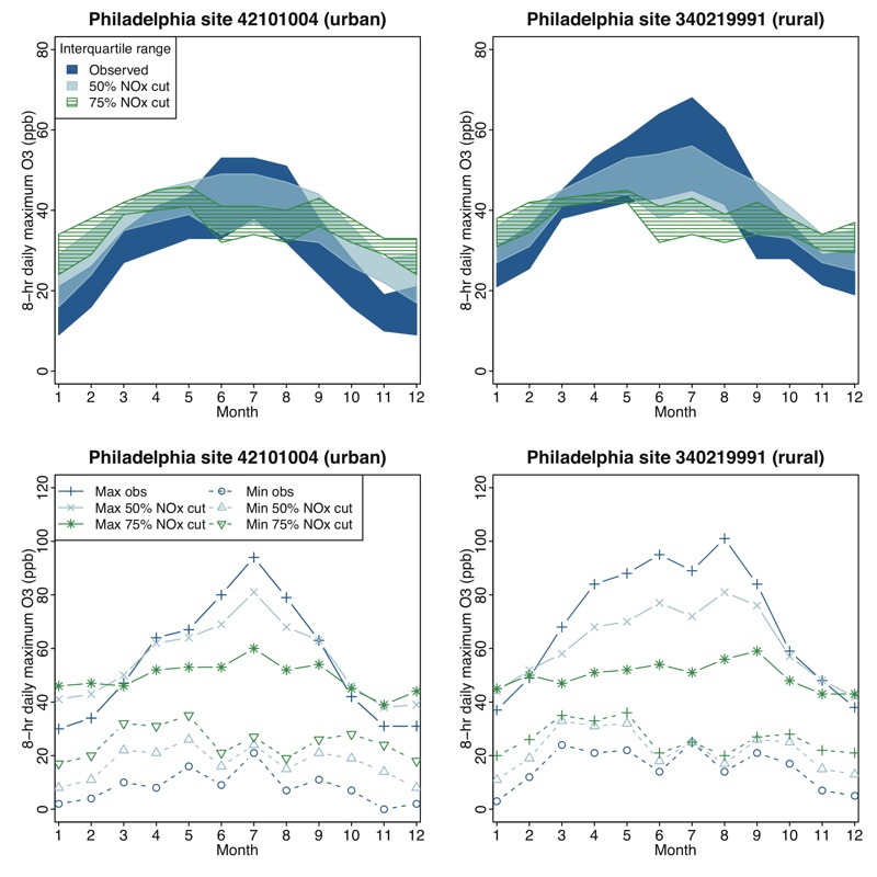
Distribution of 8-hr daily maximum ozone (O3) concentrations in Philadelphia by month at an urban (left panels) and a rural (right panels) monitoring site. Top plots show the interquartile range (25th to 75th percentile values) across all days in each month. Bottom plots show minimum and maximum values across all days in each month.
Changes in diurnal patterns at these two monitoring sites are shown in Figure S11. Nighttime concentrations were predicted to increase with decreasing NOx, whereas daytime concentrations were predicted to decrease. Similar to changes in the seasonal pattern, these changes generally led to a flattening out of the diurnal pattern. Increases were more pronounced at the urban monitor, where concentrations were low, than at the rural monitor, where concentrations were high.
Temporal plots for the other four cities showed generally similar patterns to those observed in Philadelphia and can be found in Figures S12–S19.
Discussion
Limitations and Uncertainties
We note several limitations and uncertainties. First, we looked at two scenarios of across-the-board reductions in U.S. anthropogenic NOx (and VOC) emissions as case studies to demonstrate how changing emissions could affect spatial and temporal patterns of O3. Our modeling explored broad regional reductions in NOx (and VOC) emissions, and we have not evaluated whether more spatially focused reductions could be equally effective in reducing peak concentrations while avoiding increases in O3 in urban core areas. Future research may explore strategies for mitigating NOx-related increases in O3. In addition, different sources are likely to reduce their emissions at different rates. This analysis demonstrated how spatial and temporal O3 patterns and resulting exposure may change with emissions reductions but did not attempt to predict future emissions levels or the associated effects on O3. Second, we applied modeled O3 responses from 12-km–resolution regional model simulations to ambient measurements at O3 monitors. Although 12-km–resolution modeling has generally been shown to capture most features of O3 response, the variability in predicted O3 responses can be somewhat muted compared with that found in modeling performed at finer grid resolutions (Cohan et al. 2006). Third, we note that in Philadelphia, the increasing seasonal mean values were only predicted at a single monitor, and in Chicago, increases in the regulatory metric were only predicted at two monitors. In both cases, there was some uncertainty in the VNA interpolations showing the spatial extent of those increases. Finally, this analysis used 7 months of modeling data to represent O3 responses across 3 years. The modeling simulated at least 1 representative month for each season, allowing us to create separate regressions for each site, hour of the day, and season, which enabled us to capture seasonal variability in the response of O3 to emissions changes. In addition, both meteorology (e.g., ozone-conducive conditions) and emissions in 2006 and 2008 may have varied from those in the 2007 modeling year. Therefore, the application of regressions based on conditions from 7 months in 2007 to 2006–2008 observations is another source of uncertainty.
Implications for Future Epidemiology Studies and Risk Assessments
The results from this analysis show substantial heterogeneity in O3 responses within CSAs. These findings suggest that the composite monitors used in many health studies may mask potentially important aspects of the impact of NOx changes on O3 distributions (changes to high vs. low O3 concentrations, spatial variability, and temporal patterns) and how they relate to total population-weighted exposure.
First, a key observation from our analysis is that for all three areas, O3 concentrations using the regulatory metric were reduced at locations with the highest concentrations (which are generally the monitors that are targeted when selecting NOx or VOC emissions controls). Additionally, monthly maximum O3 was decreased at both urban and rural sites under the 50% and 75% NOx cut scenarios (Figure 8). As noted earlier, some measures of risk, such as the lung function responses derived from controlled human exposure studies, are most sensitive to these reductions in high concentrations, and thus, these risk metrics will show improvement with decreases in NOx. In contrast, the epidemiology-based risks that are currently equally responsive to changes at low and high concentrations are more ambiguous in response to NOx decreases and ultimately depend on the direction and magnitude of the O3 change in places with the highest population densities. Because increases in O3 almost always occur at low O3 concentrations, it is increasingly important for health studies to evaluate whether the shape of the concentration–response relationship changes at these lower levels.
Second, spatial gradients of ambient O3 are evident in each of the urban areas shown, and there is both spatial and temporal heterogeneity in the response of ambient O3 to NOx decreases. This heterogeneity enhances the importance of understanding where and when people spend their days when linking ambient monitoring data to health outcomes. The U.S. EPA (2014a) found that when population exposures to O3 are modeled using time–activity information, the highest exposures to O3 occur for children spending a large amount of time outdoors during high-O3 periods and for adult outdoor workers in high-O3 areas. These findings suggest that epidemiology studies could be improved and that exposure misclassification could be reduced by providing population exposure surrogates that represent time–activity weighted patterns of O3 exposure instead of using simpler spatial averages or single-point measures that assume individuals spend all of their time at a residential location. In addition, time–activity weighted measures of population exposure to O3 will be better able to capture the changes in spatial and temporal patterns of O3 that can result from reductions in O3 precursor emissions to attain the NAAQS.
Third, the model predictions that increases in O3 are more prevalent in cooler months and that decreases are more prevalent in warmer months may be important if activities that lead to increased exposure (such as time spent outdoors) are practiced less frequently in winter than in summer. Some research suggests that health impacts of O3 may be lower in cooler months than in warmer months (Medina-Ramón 2006; Stieb et al. 2009; Strickland et al. 2010). To the extent that O3 health impacts vary by season, a fuller characterization of exposure patterns may improve understanding of the implications of the predicted changes in seasonal O3 patterns.
Conclusion
The net impact of emissions reductions on health over an entire population will depend on the balance of O3 changes across high- and low-population-density locations and across the entire O3 season as well as on the shape of the concentration–response relationship at different concentrations. Our analysis highlights the potential impacts of NOx emissions reductions on spatial and temporal patterns of O3. Extensions of this work that elucidate the relationships between population time–activity patterns (as well as potentially affected communities) and these changes in the spatial and temporal patterns of O3 may allow regulators to consider modifications to NOx and VOC reduction plans (e.g., to avoid increases in O3 at times and locations when they are most likely to result in negative health outcomes).
Supplemental Material
Acknowledgments
The authors would like to thank N. Possiel, A. Lamson, K. Scavo, J. Hemby, K. Bremer, and M. Koerber at the U.S. Environmental Protection Agency (EPA) for their thoughtful review and comments on this article.
Footnotes
Although this paper has been reviewed by the U.S. EPA and approved for publication, it does not necessarily reflect the U.S. EPA’s policies or views.
The authors declare they have no actual or potential competing financial interests.
References
- Bell M. The use of ambient air quality modeling to estimate individual and population exposure for human health research: a case study of ozone in the Northern Georgia Region of the United States. Environ Int. 2006;32:586–593. doi: 10.1016/j.envint.2006.01.005. [DOI] [PubMed] [Google Scholar]
- Cai C, Kelly JT, Avise JC, Kaduwela AP, Stockwell WR. Photochemical modeling in California with two chemical mechanisms: model intercomparison and response to emission reductions. J Air Waste Manag Assoc. 2011;61:559–572. doi: 10.3155/1047-3289.61.5.559. [DOI] [PubMed] [Google Scholar]
- Chameides WL, Lindsay RW, Richardson J, Kiang CS. The role of biogenic hydrocarbons in urban photochemical smog: Atlanta as a case study. Science. 1988;241:1473–1475. doi: 10.1126/science.3420404. [DOI] [PubMed] [Google Scholar]
- Chen J, Zhao R, Li Z. Voronoi-based k-order neighbour relations for spatial analysis. ISPRS J Photogramm Remote Sens. 2004;59:60–72. [Google Scholar]
- Cleveland WS, Graedel TE. Photochemical air pollution in the northeast United States. Science. 1979;204:1273–1278. doi: 10.1126/science.204.4399.1273. [DOI] [PubMed] [Google Scholar]
- Clifton OE, Fiore AM, Correa G, Horowitz LW, Naik V. Twenty-first century reversal of the surface ozone seasonal cycle over the northeastern United States. Geophys Res Lett. 2014;41:7343–7350. [Google Scholar]
- Cohan DS, Hu Y, Russell AG. Dependence of ozone sensitivity analysis on grid resolution. Atmos Environ. 2006;40:126–135. [Google Scholar]
- Gold C, Remmele PR, Roos T. In: Algorithmic Foundation of Geographic Information Systems. In: Lecture Notes in Computer Science, Vol. 1340 (van Kereveld M, Nievergelt J, Roos T, Widmayer P, eds) Berlin, Germany: Springer-Verlag; 1997. Voronoi methods in GIS. pp. 21–35. [Google Scholar]
- Hakami A, Odman MT, Russell AG. High-order, direct sensitivity analysis of multidimensional air quality models. Environ Sci Technol. 2003;37:2442–2452. doi: 10.1021/es020677h. [DOI] [PubMed] [Google Scholar]
- Hogrefe C, Hao W, Zalewsky E, Ku JY, Lynn B, Rosenzweig C, et al. An analysis of long-term regional-scale ozone simulations over the Northeastern United States: variability and trends. Atmos Chem Phys. 2011;11:567–582. [Google Scholar]
- Jerrett M, Burnett RT, Pope CA, III, Ito K, Thurston G, Krewski D, et al. Long-term ozone exposure and mortality. N Engl J Med. 2009;360:1085–1095. doi: 10.1056/NEJMoa0803894. [DOI] [PMC free article] [PubMed] [Google Scholar]
- Jhun I, Coull BA, Zanobetti A, Koutrakis P. The impact of nitrogen oxides concentration decreases on ozone trends in the USA. Air Qual Atmos Health. 2015;8:283–292. doi: 10.1007/s11869-014-0279-2. [DOI] [PMC free article] [PubMed] [Google Scholar]
- Kelly JT, Baker KR, Napelenok SL, Roselle SJ. Examining single-source secondary impacts estimated from brute-force, decoupled direct method, and advanced plume treatment approaches. Atmos Environ. 2015;111:10–19. [Google Scholar]
- Kumar N, Russell AG. Multiscale air quality modeling of the Northeastern United States. Atmos Environ. 1996;30:1099–1116. [Google Scholar]
- Medina-Ramón M, Zanobetti A, Schwartz J. 2006. The effect of ozone and PM10 on hospital admissions for pneumonia and chronic obstructive pulmonary disease: a national multicity study. Am J Epidemiol 163 579 588, doi: 10.1093/aje/kwj078 [DOI] [PubMed] [Google Scholar]
- Marshall JD, Nethery E, Brauer M. Within-urban variability in ambient air pollution: comparison of estimation methods. Atmos Environ. 2008;42:1359–1369. [Google Scholar]
- Murphy JG, Day DA, Cleary PA, Wooldridge PJ, Millet DB, Goldstein AH, et al. The weekend effect within and downwind of Sacramento – part 1: observations of ozone, nitrogen oxides, and VOC reactivity. Atmos Chem Phys. 2007;7:5327–5339. [Google Scholar]
- Seinfeld JH, Pandis SN. New York: John Wiley and Sons, Inc. 1326; 1998. Atmospheric Chemistry and Physics from Air Pollution to Climate Change. [Google Scholar]
- Sillman S. The relation between ozone, NOx and hydrocarbons in urban and polluted rural environments. Atmos Environ. 1999;33:1821–1845. [Google Scholar]
- Simon H, Baker KR, Akhtar F, Napelenok SL, Possiel N, Wells B, et al. A direct sensitivity approach to predict hourly ozone resulting from compliance with the National Ambient Air Quality Standard. Environ Sci Technol. 2013;47:2304–2313. doi: 10.1021/es303674e. [DOI] [PubMed] [Google Scholar]
- Simon H, Baker KR, Phillips S. Compilation and interpretation of photochemical model performance statistics published between 2006 and 2012. Atmos Environ. 2012;61:124–139. [Google Scholar]
- Simon H, Reff A, Wells B, Xing J, Frank N. Ozone trends across the United States over a period of decreasing NOx and VOC emissions. Environ Sci Technol. 2015;49:186–195. doi: 10.1021/es504514z. [DOI] [PubMed] [Google Scholar]
- Smith RL, Xu B, Switzer P. Reassessing the relationship between ozone and short-term mortality in U.S. urban communities. Inhal Toxicol. 2009;21(suppl 2):37–61. doi: 10.1080/08958370903161612. [DOI] [PubMed] [Google Scholar]
- Stieb DM, Szyszkowicz M, Rowe BH, Leech JA. 2009. Air pollution and emergency department visits for cardiac and respiratory conditions: a multi-city time-series analysis. Environ Health 8 25, doi: 10.1186/1476-069X-8-25 [DOI] [PMC free article] [PubMed] [Google Scholar]
- Strickland MJ, Darrow LA, Klein M, Flanders WD, Sarnat JA, Waller LA, et al. 2010. Short-term associations between ambient air pollutants and pediatric asthma emergency department visits. Am J Respir Crit Care Med 182 307 316, doi: 10.1164/rccm.200908-1201OC [DOI] [PMC free article] [PubMed] [Google Scholar]
- U.S. EPA (U.S. Environmental Protection Agency) Research Triangle Park, NC: U.S. EPA. EPA-452/R-12-005; 2012. Regulatory Impact Analysis for the Final Revision to the National Ambient Air Quality Standards for Particulate Matter. http://www.epa.gov/ttnecas1/regdata/RIAs/finalria.pdf [accessed 15 October 2015] [Google Scholar]
- U.S. EPA 2013. Integrated Science Assessment for Ozone and Related Photochemical Oxidants (Final Report). Washington, DC: U.S. EPA. EPA/600/R-10/076F; http://ofmpub.epa.gov/eims/eimscomm.getfile?p_download_id=511347 [accessed 15 October 2015]. [Google Scholar]
- U.S. EPA. U.S. Environmental Protection Agency, Research Triangle Park, NC: U.S. EPA. EPA-452/R-14-004a; 2014a. Ozone (O3) Standards – Documents from Current Review – Risk and Exposure Assessments. Available: http://www.epa.gov/ttn/naaqs/standards/ozone/s_o3_2008_rea.html [accessed 15 October 2015] [Google Scholar]
- U.S. EPA. Research Triangle Park, NC: U.S. EPA. EPA-452/P-14-006; 2014b. Regulatory Imact Analysis of the Proposed Revisions to the National Ambient Air Quality Standards for Ground-Level Ozone. Available: http://www.epa.gov/ttn/ecas/regdata/RIAs/20141125ria.pdf [accessed 15 October 2015] [Google Scholar]
- Xiao X, Cohan DS, Byun DW, Ngan F. 2010. Highly nonlinear ozone formation in the Houston region and implications for emission controls. J Geophys Res 115 D23309, doi: 10.1029/2010JD014435 [DOI] [Google Scholar]
- Zanobetti A, Schwartz J. Mortality displacement in the association of ozone with mortality: an analysis of 48 cities in the United States. Am J Respir Crit Care Med. 2008;177:184–189. doi: 10.1164/rccm.200706-823OC. [DOI] [PubMed] [Google Scholar]
Associated Data
This section collects any data citations, data availability statements, or supplementary materials included in this article.