Permutation Testing for Treatment-Covariate Interactions and Subgroup Identification

Abstract

We consider the problem of using permutation-based methods to test for treatment-covariate interactions from randomized clinical trial data. Testing for interactions is common in the field of personalized medicine, as subgroups with enhanced treatment effects arise when treatment-by-covariate interactions exist. Asymptotic tests can often be performed for simple models, but in many cases, more complex methods are used to identify subgroups, and non-standard test statistics proposed, and asymptotic results may be difficult to obtain. In such cases, it is natural to consider permutation-based tests, which shuffle selected parts of the data in order to remove one or more associations of interest; however, in the case of interactions, it is generally not possible to remove only the associations of interest by simple permutations of the data. We propose a number of alternative permutation-based methods, designed to remove only the associations of interest, but preserving other associations. These methods estimate the interaction term in a model, then create data that “looks like” the original data except that the interaction term has been permuted. The proposed methods are shown to outperform traditional permutation methods in a simulation study. In addition, the proposed methods are illustrated using data from a randomized clinical trial of patients with hypertension.

1 Introduction

In clinical trials, a common goal is to search for subgroups of enhanced treatment effect. A well-known risk in subgroup analysis is that of false positives (Yusuf et al, 1991; Peto et al, 1995; Assmann et al, 2000; Brookes et al, 2001). One way to reduce this risk is to pre-define a small number of potential subgroups before looking at the data; however, one may not always know a priori which subgroups may be of interest. When considering pre-defined subgroups, one common approach to reducing the risk of false positive findings is to consider a multiple testing procedure, such as a Bonferroni correction. Multiple testing procedures can effectively reduce false positives, but generally also lack power to detect true subgroups. Thus, one may instead wish to pre-define a statistical approach for identifying subgroups (Ruberg et al, 2010), which can be implemented using the data (Cai et al, 2011; Foster et al, 2011; Lipkovich et al, 2011; Zhang et al, 2012). Such pre-defined approaches can be very effective, but may still be prone to false discoveries (Foster et al, 2011). To help quantify the potential usefulness of identified subgroups, Foster et al (2011) considered the use of a metric, Q(A), which is defined as the difference between the expected treatment effect in some subset of the covariate space, denoted A, and the overall treatment effect. Such a metric can also be helpful for eliminating false subgroups, as small values suggest a lack of enhancement, but may be more effective if one can also obtain p-values for the metric estimates.

Before obtaining a p-value, one must consider what “null” means in a particular setting. Subgroups of enhanced (or more generally, different) treatment effect occur when the effect of treatment depends on the covariate values, i.e., such subgroups arise when treatment-by-covariate interactions exist. Thus, in this setting, “null” data may be defined as data in which no treatment-by-covariate interactions exist. Alternatively, if one has implemented a subgroup identification procedure, and wishes to evaluate the identified region of the covariate space, A, null data could be defined as data for which the treatment effect in region A is equal to the overall treatment effect. In this paper, we will focus on the more general null scenario that no treatment-by-covariate interactions exist.

Consider the following general model:

$$y_i=h({\mathit{x}}_i)+g({\mathit{x}}_i)(T_i-\pi )+{\mathit{\in }}_i,$$ (1.1)

where y_i is the observed continuous outcome measure for subject i, x_i is the i^th row of the standardized n × p covariate matrix X, and T_i is a binary indicator of which treatment subject i received. Additionally, ε_i, i = 1, …, n are independent and identically distributed (iid) errors with mean zero and variance σ² which are independent of the covariates, and π is the treatment randomization probability for T = 1. We wish to consider a general class of models, so h and g are unspecified. Note that in this model, g(x_i) is the treatment effect at covariate value x_i. Our goal is to test the null hypothesis that g(x) is constant with respect to the covariates x. That is, we wish to test for treatment-by-covariate interactions. One possible approach is to develop a test statistic for which asymptotic properties can be obtained, but this may be difficult for more general methods. In such cases, a common approach is to use permutation tests.

A number of authors, including Edgington (1986); Good (2000); Potthoff et al (2001); Bůžková et al (2011) and Simon and Tibshirani (2012), have considered the testing of interactions using more traditional permutation-based methods, which work by shuffling parts of the data, such as the outcome, some or all of the covariates, or the treatment indicators, with the goal of eliminating one or more specific associations. In general, permutations shuffle selected parts of the data set in such a way that the new data “look like” the original data in some aspects, but in other aspects, the new data differ from the original data. For example, marginal distributions are preserved, but some associations between selected variables are not preserved. With simple permutations, such as permuting the treatment group indicator, it may not be possible to completely control which aspects of the original data are preserved, and which are changed. An issue which must be addressed if one wishes to test for interactions using permutation-based methods is that it is generally impossible to remove only the associations of interest by simple permutations the data. One way to reduce the drawbacks of removing more than just the association of interest is to “cleverly” choose a test statistic (Edgington, 1986; Good, 2000; Potthoff et al, 2001; Bůžková et al, 2011), but there may not always be an obvious choice.

In this paper, we have a broad definition of what a permuted data set is. The “permutation-like” methods that we will develop and describe later in this paper have a similar characteristic of preserving some aspects of the data structure, while not preserving other aspects, but in a somewhat more controlled fashion. In particular, we will propose alternative forms of permutation methods, which are designed to remove only the associations of interest, thereby avoiding some of the potential issues with using traditional permutation tests for interactions.

The remainder of this paper is as follows. In Section 2 we briefly review permutation tests and present a variety of alternative methods for obtaining p-values. In Section 3, the proposed methods are compared with a number of commonly-used permutation-based approaches in a simulation study. In Section 4, the proposed methods are implemented on real data from a randomized clinical trial, and in Section 5 we present a discussion.

2 Permutation tests

2.1 Review of permutation tests

Suppose we have observed data (y₁, x₁), …, (y_n, x_n), where y is some outcome and x is a covariate of interest, and that we only consider testing the null hypothesis of no association between y and x. This is generally done by calculating a test statistic, say $\widehat{\mathit{TS}}$, and then obtaining a p-value based on the null distribution of $\widehat{\mathit{TS}}$. In lieu of using asymptotics to determine the null distribution of $\widehat{\mathit{TS}}$, one may wish to employ a permutation test. For testing the null hypothesis that no association exists between x and y, approximately “null” data can be obtained by permuting either x or y. This is essentially the same as replacing the permuted covariate with a randomly generated noise covariate of the same distribution. Permutation tests work by repeating the process many times (say K), each time calculating a new value of the test statistic, ${\widehat{\mathit{TS}}}^{(k)}$. These K values are then used to define an approximated null distribution for $\widehat{\mathit{TS}}$, from which a p-value can be obtained.

As noted by Edgington (1986), there are two basic methods of permuting data. One approach is the systematic method, in which all possible permutations are considered; however, in this case, K = n! (if the observed values are unique), so for even moderate sample sizes, the number of possible permutations will be very large. An alternative approach is random or Monte Carlo permutation, in which only a random subset of the possible permutations are considered, making it much more feasible for moderate-to-large data sets. In this paper, we consider only random permutation tests.

In the next subsection, we consider several methods which are permutation based, but are specifically designed to test only for interactions, which is something traditional permutation tests are generally unable to do. Though the proposed methods could be applied to any interaction, we will limit our discussion to treatment-by-covariate interactions.

2.2 Modified permutation methods

Traditional permutation tests may not be ideal if one wishes to test for interactions, as they will generally be unable to remove only the association of interest. To better understand why this is, consider the following example. Suppose we have data from a randomized clinical trial (RCT) (y_i, T_i, x_i), i = 1, …, n, and that we wish to fit the interaction model y_i = β₀ + β^T xi + γ(T_i −π) + θ^T x_i (T_i −π) + ε_i, where β and θ are p × 1. In particular, suppose we wish to test for an interaction between treatment and one covariate, say x_j. That is, we wish to test the null hypothesis θ_j = 0. Permuting y will eliminate the desired interaction, but will also eliminate all main effects of the covariates and the treatment, thereby making the “true” underlying model $y_i={\beta }_0+{{\mathit{\in }}^{\prime }}_i$. Similarly, permuting the covariate x_j or the treatment indicator T will eliminate the interaction, but also the corresponding main effect for either x_j or T, leading to a “true” underlying model where β_j = θ_j = 0 or γ = 0, θ = 0 respectively. For certain test statistics (such as those which are pivotal), the impact of removing these additional associations can be greatly reduced (Edgington, 1986; Good, 2000; Potthoff et al, 2001; Bůžková et al, 2011), but in many situations such statistics may not be apparent.

One simple way to address this issue is considered by Potthoff et al (2001), and involves permuting the covariates of interest within levels of T. Thus, in this case, one would permute values of x_j separately for those with T = 1 and those with T = 0. This approach will avoid removing the main effect for treatment, but still eliminates the main effect for x_j, so that the null model has β_j = θ_j = 0. Note that if one wishes to test for all x-by-T interactions (null hypothesis θ = 0), this approach is equivalent to permuting y within levels of T.

Consider now the general model (1.1), and suppose we are interested in testing whether or not the treatment effect, g(x_i), is constant with respect to the covariates x_i. Additionally, suppose that model (1.1) has been fitted, giving function estimates ĥ and ĝ, and let $\widehat{\mathit{TS}}$ be the sample value of the test statistic of interest. Our methods are designed to perturb the values of ĝ(x_i) to obtain a new treatment effect, $g_i^{\ast }$, which does not depend on the covariates (details will be discussed later). Using this null treatment effect, along with the specific form of model (1.1), we obtain p-values as follows:

1. Create a new “null” outcome, $y_i^{\ast (k)}=\widehat{h}({\mathit{x}}_i)+g_i^{\ast }(T_i-\pi )+{\stackrel{\sim }{e}}_i^{(k)}$, i = 1, …, n, where ${\stackrel{\sim }{e}}_1^{(k)},\dots ,{\stackrel{\sim }{e}}_n^{(k)}$ are randomly sampled (without replacement) centered residuals from fitted model (1.1).

2. Use y*^(k), X and T to refit model (1.1), and obtain a new value of the test statistic, ${\widehat{\mathit{TS}}}^{(k)}$.

3. Repeat steps 1 and 2 K times (i.e. k = 1, …, K) to yield K values of the test statistic, and use these values to obtain an approximate null distribution for the test statistic.

4. Use this approximate null distribution and the test statistic value from the observed data, $\widehat{\mathit{TS}}$ to obtain a p-value (either one or two-sided).

We now consider methods which use the estimated treatment effect, ĝ, to obtain the null treatment effect, g*.

A. Mean of estimated treatment effect

1. Fixed g* approach: Perhaps the simplest null scenario in this setting is that of a constant treatment effect for all individuals. Thus, one natural choice is to create null data by giving all individuals the average estimated treatment effect, so that $g_i^{\ast }=\frac{1}{n}{\displaystyle {\sum }_{i=1}^n\widehat{g}({\mathit{x}}_i)}\equiv \overline{\widehat{g}}$, i = 1, …, n. For the remainder of this paper, this will be referred to as the fixed g* approach.

2. Fixed g* (RN) approach: One could also consider a variation of the fixed g* case, in which individuals have treatment effects which vary randomly around a fixed, population-wide mean. In this case, we define the null treatment effect for subject i to be $g_i^{\ast }=\overline{\widehat{g}}+{\stackrel{\sim }{\mathit{\in }}}_{g,i}$, where ${\stackrel{\sim }{\mathit{\in }}}_g$ is a random permutation of the residuals $\widehat{\mathit{g}}-\overline{\widehat{g}}$. This will be referred to as the fixed g* random noise, or fixed g* (RN) approach.

3. Fixed g* (BN) approach: Alternatively, if one has reason to believe these residuals do not vary equally about $\overline{\widehat{g}}$ for all subjects, one may instead consider $g_i^{\ast }=g_{i,\mathit{Bern}}^{\ast }=\overline{\widehat{g}}+{\mathit{\in }}_{g,\mathit{Bern},i}$, where ${\mathit{\in }}_{g,\mathit{Bern},i}=\{\begin{array}{cc}{\widehat{g}}_i-\overline{\widehat{g}}& \text{when}a=1\\ {\overline{\widehat{g}}}_i-\widehat{g}& \text{when}a=0\end{array}$, and a is an independently generated Bernoulli $\left(\frac{1}{2}\right)$ random variable. This will be referred to as the fixed g* Bernoulli noise, or fixed g* (BN) approach.

B. Randomly shuffled estimated treatment effect

1. Random g* approach: As an alternative to the fixed treatment effect case, one may wish to consider a scenario in which each subject’s response to treatment is random, but does not depend on the covariates. Therefore, we could also consider creating null data by giving each individual a random estimated treatment effect, so that $g_i^{\ast }={\stackrel{\sim }{g}}_i$, where ĝ is a random permutation of the estimated treatment effects. Note that this method is actually identical to the fixed g* (RN) approach. Thus, we will not consider them separately.

2. Random g* (RN) approach: As with the fixed g* approach, one could also consider the addition of random noise to the random treatment effects, ĝ. This could be done by following an approach similar to that used in the fixed g* method. Specifically, we may consider $g_i^{\ast }={\stackrel{\sim }{g}}_i+{\stackrel{\sim }{\mathit{\in }}}_{g,i}$, where ${\stackrel{\sim }{\mathit{\in }}}_g$ is as defined above in A(2). This will be referred to as the random g* random noise, or random g* (RN) approach. We will also consider a modified version of this approach, where y* is obtained by adding randomly sampled g* residuals, y – ĥ – g* (T − π), to ĥ + g* (T − π), instead of randomly sampled residuals from model (1.1). This will be referred to as the random g* (RN) (g* Residual) approach.

3. Random g* (BN) approach: Alternatively, we may consider $g_i^{\ast }={\stackrel{\sim }{g}}_{i,\mathit{Bern}}^{\ast }$, where ${\stackrel{\sim }{g}}_{\mathit{Bern}}^{\ast }$ is a random permutation of ${\stackrel{\sim }{\mathit{g}}}_{\mathit{Bern}}^{\ast }$ (defined above in A(3)). This will be referred to as the random g* Bernoulli noise, or random g*(BN) approach. We will also consider a modified version of this approach, where y* is obtained by adding randomly sampled g* residuals, y – ĥ – g* (T − π), to ĥ + g* (T − π), instead of randomly sampled residuals from model (1.1). This will be referred to as the random g* (BN) (g* Residual) approach.

C. Constrained least-squares approach

One may also consider obtaining null data by modifying the estimated treatment effects so that they are approximately null, but with similar values to the original estimates. To do this, we use least squares to calculate an approximate treatment effect, $g_i^{\ast }$, which is close to ĝ(x_i), but has marginal sample correlations of zero with all the covariates. That is, we choose values $g_i^{\ast }$, i = 1, …, n which minimize

$${\displaystyle \sum _{i=1}^n{\{\widehat{g}({\mathit{x}}_i)-g_i^{\ast }\}}^2}$$

under the constraint that the sample correlations between g* and x_j, j = 1, …, p, are zero, or equivalently by minimizing

$${\displaystyle \sum _{i=1}^n{\{\widehat{g}({\mathit{x}}_i)-g_i^{\ast }\}}^2}+{\displaystyle \sum _{j=1}^p{\lambda }_j}{\displaystyle \sum _{i=1}^n{g}_i^{\ast }{x}_{ij}}$$

with respect to g*, where λ_j, j = 1, …, p, are Lagrange multipliers. Note that if the covariates are not centered, the penalty term becomes ${\displaystyle {\sum }_{j=1}^p{\lambda }_j}{\displaystyle {\sum }_{i=1}^n(g_i^{\ast }-{\overline{g}}^{\ast })(x_{ij}-{\overline{x}}_j)}$. It is straightforward to show that the minimizer satisfies

$$\begin{array}{c}\mathit{g}\ast =\widehat{\mathit{g}}-\frac{1}{2}\mathit{X}\mathit{\lambda },\\ \text{where}\mathit{\lambda }=2{({\mathit{X}}^T\mathit{X})}^{-1}{\mathit{X}}^T\widehat{\mathit{g}}.\end{array}$$ (2.1)

This method will be referred to as the Lagrange g* approach. It should be noted that a correlation of zero between the treatment effect and a co-variate does not necessarily mean the treatment effect is independent of the covariate. Though we do not discuss it here, one could also consider additional constraints, such as g* being uncorrelated with $x_j^2$, or g* being uncorrelated with ĥ. To better understand why the Lagrange method should work, note that g* is exactly equal to the residuals from the model $\widehat{g}({\mathit{x}}_i)={\mathit{x}}_i^T\mathit{\omega }+{\mathit{\in }}_i$. Thus, the Lagrange method works by estimating the contribution of the covariates to the treatment effect, and then removing this estimated contribution, so that only the part of the estimated treatment effect that does not depend on the covariates remains. We will also consider a modified version of this approach, where y* is obtained by adding randomly sampled g* residuals, y – ĥ – g* (T − π), to ĥ + g* (T − π), instead of randomly sampled residuals from model (1.1). This will be referred to as the Lagrange g* (g* Residual) approach.

3 Simulations

To evaluate the performance of the proposed methods under a variety of scenarios, a simulation study was performed. In addition to the proposed methods, we considered four permutation-based methods:

• –Permutation of y;
• –Permutation of X;
• –Permutation of T;
• –Permutation of y within levels of T.

These approaches will be referred to as the permute y, permute X, permute T and permute y (in T) methods respectively. We begin by considering a linear model with treatment-by-covariate interactions, which allows us to compare the proposed methods to both permutation and exact p-values. We then discuss simulation results for a subgroup identification procedure, based on a more complex model.

3.1 Simple linear model example

Data were generated from the model

$$y=3+{\mathit{\beta }}^T\mathit{x}+\gamma (T-\frac{1}{2})+{\mathit{\theta }}^T\mathit{x}(T-\frac{1}{2})+\mathit{\in },$$

where ε’s and all x’s are iid standard normal, and the design matrix, X, has five columns. The true parameter values are β = (β₁, 0, β₁, 0, β₁)^T, and θ = (θ₁, θ₁, 0, 0, 0)^T. Thus, only x₁, x₃ and x₅ have true nonzero main effects (which are equal), and only x₁ and x₂ have true nonzero interactions with treatment (which are equal). Because these parameter values would not generally be known to us, we assume that all five covariates have unique, nonzero main effects and interactions with treatment when fitting the model. In this case, the test of interest (for the assumed model, given below) is that θ_j = 0, j = 1, …, 5. This is a situation where the F statistic has a known distribution, and thus an exact test exists. We considered four scenarios:

• θ₁ = 0.35, γ = 0.25, β₁ = 0.5;

• θ₁ = 0, γ = 0.25, β₁ = 0.5;

• θ₁ = 0.35, γ = 0.5, β₁ = 0.25;

• θ₁ = 0, γ = 0.5, β₁ = 0.25.

In scenarios (1) and (2), the main effects for the covariates are large, and in scenarios (3) and (4) the main effect for treatment is large. These cases were chosen to illustrate the potential shortcomings of traditional permutation-based tests when large main effects exist. In each scenario, 500 data sets of size 200 were generated, and the model $y=\alpha +{\mathit{\beta }}^T\mathit{x}+\gamma \left(T-\frac{1}{2}\right)+{\mathit{\theta }}^T\mathit{x}\left(T-\frac{1}{2}\right)+\mathit{\in }$ (vs. was fitted. The null hypothesis was that no x-by-T interactions exist (vs. alternative that at least one exists). To assess the sensitivity of the methods to the choice of test statistic, we computed the permutation p-values using an F statistic and also the statistic ${\displaystyle \sum {\widehat{\theta }}_j^2}$, which was chosen because it is somewhat “ad hoc.” For all non-asymptotic methods, 1000 permutations were used (so K = 1000).

Note that, in this case, the covariates are independent, as are the observations, and the design matrix is standardized. As a result, it can be shown that X (X^T X)⁻¹X^T is approximately equal to $\left(\frac{p}{n}\right)\mathit{I}$, where I is an n × n identity matrix. For the fitted model, the estimated treatment effect vector ĝ is equal to $\widehat{\mathit{\gamma }}+\mathit{X}\widehat{\mathit{\theta }}$, where $\widehat{\mathit{\gamma }}={(\widehat{\gamma },\dots \widehat{\gamma })}^T$. Thus for the Lagrange method, from (2.1) we have g* method, we have

$$\begin{array}{l}\mathit{g}\ast =\widehat{\mathit{g}}-\mathit{X}{({\mathit{X}}^T\mathit{X})}^{-1}{\mathit{X}}^T\widehat{\mathit{g}}\\ =\widehat{\mathit{\gamma }}+\mathit{X}\widehat{\mathit{\theta }}-\mathit{X}{({\mathit{X}}^T\mathit{X})}^{-1}{\mathit{X}}^T\widehat{\mathit{\gamma }}-\mathit{X}{({\mathit{X}}^T\mathit{X})}^{-1}{\mathit{X}}^T\mathit{X}\widehat{\mathit{\theta }}\\ =\widehat{\mathit{\gamma }}+\mathit{X}\widehat{\mathit{\theta }}-\mathit{X}{({\mathit{X}}^T\mathit{X})}^{-1}{\mathit{X}}^T\widehat{\mathit{\gamma }}-\mathit{X}\widehat{\mathit{\theta }}\\ =(\mathit{I}-\mathit{X}{({\mathit{X}}^T\mathit{X})}^{-1}{\mathit{X}}^T\widehat{\mathit{\gamma }}\\ \approx \left(1-\frac{p}{n}\right)\widehat{\mathit{\gamma }}\approx \widehat{\mathit{\gamma }},\end{array}$$

where the last approximation is a result of the fact that, in this case, p is considerably smaller than n, so that $\frac{p}{n}$ is nearly zero. In addition, for the fixed g* method, we have

$$g_i^{\ast }=\frac{1}{2}{\displaystyle \sum _i(\widehat{\gamma }+{\mathit{x}}_i^T\widehat{\mathit{\theta }})}=+\frac{1}{n}{\displaystyle \sum _j\left({\widehat{\theta }}_j{\displaystyle \sum _i{x}_{ij}}\right)=\widehat{\gamma },}$$

again because covariates are standardized, so that the second term is exactly zero. Therefore, for this specific example, the Lagrange and fixed g* methods are nearly identical. Note that if the covariates were correlated, the o -diagonal elements of X (X^T X)⁻¹ X^T would be non-zero, leading to unique Lagrange g* values for each subject. Thus, in this case the Lagrange and Fixed g* methods would be different.

Looking at Figure 1, we can see that rejection rates when using the F statistic are generally similar for all methods in all four scenarios, whereas the rejection rates for the statistic ${\displaystyle \sum {\widehat{\theta }}_j^2}$ vary noticeably between methods. In particular, the ${\displaystyle \sum {\widehat{\theta }}_j^2}$ rejection rates for the permute X, permute y and permute y (in T) methods tend to be considerably lower than those for the other methods. This is due to the fact that these methods remove several main effects (in addition to the desired interactions) in the process of creating new “null” outcome values, which subsequently have larger error variances than the observed outcome values. Because ${\displaystyle \sum {\widehat{\theta }}_j^2}$ comes from the parameter estimates for a linear regression model, its variance depends on the variance of the outcome values, and in particular will increase or decrease as the error variance of the outcome increases or decreases. Thus, the permute X, permute y and permute y (in T) methods induce “null” distributions for ${\displaystyle \sum {\widehat{\theta }}_j^2}$ which have much larger variances than the correct null distribution (where only the interactions are removed), leading to larger p-values and fewer rejections. A similar effect can be seen in the permute T method, but to a lesser degree, as this method only removes one main effect. This is also somewhat of a problem for the Random g* (RN) and Random g* (BN) approaches, particularly when g*-based residuals are used to obtain y*. In contrast, the Lagrange and Fixed g* methods create “null” outcome values whose variances are slightly smaller than that of the observed outcome values, causing these methods to give elevated rejection rates. For the Lagrange method, using g*-based residuals to obtain y* noticeably reduces this problem. This general phenomenon is mentioned by Bůžková et al (2011), who note that permutation-based methods perform better for statistics with a pivotal null distribution.

Fig. 1.

Rejection rates (α = 0.05) for simple linear model simulations

Among the proposed methods, the Fixed g* (BN), Fixed g* (RN) and Lagrange (g* Residuals) approaches perform best, followed by the Random g* (RN) and Random g* (BN) methods, which also performed reasonably well. The Fixed g* and Lagrange g* approaches had good power, but had elevated type-I error rates for the ad hoc test statistic. The Random g* (RN) (g* residuals) and Random g* (BN) (g* residuals) methods performed worst among the proposed methods, showing lower power and very conservative type-I error rates for the ad hoc test statistic. Overall, the best methods (not based on the exact F distribution) are fixed g* (BN), fixed g* (RN) and Lagrange (g* Residuals) approaches, which have rejection rates that are nearly identical for both the F statistic and ${\displaystyle \sum {\widehat{\theta }}_j^2}$, and which are very close to 0.05 in the “null” scenarios (2 and 4).

Figure 2 further illustrates the effect of creating “null” data which has an outcome error variance that is too large (or too small). This is again most noticeable for the permute X, permute y and permute y (in T), methods, whose histograms are obviously non-uniform. The histograms for these three methods were also found to have considerably heavier right tails in the non-null scenarios (1 and 3) (results not shown). We can also see that the use of g*-based residuals to obtain y* appears to lead to a more uniform distribution of p-values for the Lagrange approach. The results for the statistic ${\displaystyle \sum {\widehat{\theta }}_j^2}$ help illustrate the importance of an appropriately chosen permutation method when the test statistic is somewhat ad hoc, as may be the case in situations where asymptotics are difficult to obtain.

Fig. 2.

Histograms of p-values for simple linear scenario 2 (β₁ = 0.5, γ = 0.25, θ₁ = 0)

3.2 Complex model example

As mentioned previously, the proposed methods were motivated by our interest in subgroup analysis. We now discuss simulations in which the proposed methods are applied to a subgroup identification procedure (Foster et. al, 2014, to appear in Biostatistics).

3.2.1 Methods and test statistics

The subgroup identification procedure considered in this simulation study consists of two stages, and is designed to identify the simple subgroup,  which, if used to assign treatment (i.e. subjects in  get treatment, those in Â^c get control), gives the largest expected response (among candidate subgroups). In stage 1, we use nonparametric regression to obtain the estimated treatment effect, ĝ(x_i), for each subject. In stage 2, these estimated treatment effects are used to evaluate many one, two and three-dimensional regions of the general form $\left\{x_{ij}\frac{>}{<}{c}_j\right\}$, or $\left\{x_{ij}\frac{>}{<}{c}_j\right\}\cap \left\{x_{ik}\frac{>}{<}{c}_k\right\}$ or $\left\{x_{ij}\frac{>}{<}{c}_j\right\}\cap \left\{x_{ik}\frac{>}{<}{c}_k\right\}\cap \left\{x_{il}\frac{>}{<}{c}_l\right\}$, where ⋛ indicates either ≥ or < and covariates j, k and l are distinct. For each candidate subgroup, we compute the estimated expected outcome under a treat-if-in-subgroup regime. The subgroup which maximizes this estimated expected outcome is then selected. This approach will be referred to as simple optimal regime approximation (SORA).

Once  is identified, its enhancement is assessed using the following metric from Foster et al (2011):

$$Q(\widehat{A})=E(y|T=1,\mathit{x}\in \widehat{A})-E(y|T=0,\mathit{x}\in \widehat{A})-[E(y|T=1)-E(y|T=0)],$$

which can be viewed as the treatment effect enhancement in the region  beyond the overall treatment effect. We are interested in testing whether or not the identified subgroup is “real,” so the null hypothesis is that Q(Â) is 0 (vs. alternative that Q(Â) > 0). Four estimates of Q(Â) are used as test statistics for the proposed methods. The first statistic, denoted $\widehat{Q}{(\widehat{A})}_{\mathit{RS}}$, is obtained by subtracting the observed marginal treatment effect from the observed treatment effect in the region Â:

$$\begin{array}{c}\widehat{Q}{(\widehat{A})}_{\mathit{RS}}=\left(\frac{{\displaystyle {\sum }_i{y}_i{T}_{i}I({\mathit{x}}_i\in \widehat{A})}}{{\displaystyle {\sum }_i{T}_{i}I({\mathit{x}}_i\in \widehat{A})}}-\frac{{\displaystyle {\sum }_i{y}_i(1-T_i)I({\mathit{x}}_i\in \widehat{A})}}{{\displaystyle {\sum }_i(1-T_i)I({\mathit{x}}_i\in \widehat{A})}}\right)-\\ \left(\frac{{\displaystyle {\sum }_i{y}_i{T}_i}}{{\displaystyle {\sum }_i{T}_i}}-\frac{{\displaystyle {\sum }_i{y}_i(1-T_i)}}{{\displaystyle {\sum }_i(1-T_i)}}\right).\end{array}$$

This is expected to be positively biased, as the same data which were used to identify the region  are being used to estimate Q(Â).

Note that independent outcome values from approximately the same distribution could be obtained by adding random residuals to the outcome estimates, ŷ. Thus, one way to reduce the bias of $\widehat{Q}{(\widehat{A})}_{\mathit{RS}}$ is to obtain independent outcome measures as described above, and use these instead of y_i’s to compute $\widehat{Q}{(\widehat{A})}_{\mathit{RS}}$. This could be repeated several times, and the resulting estimates could be averaged to obtain a less biased estimate of Q(Â); however, because the residuals have mean zero, this is approximately equivalent to replacing the observed y values with ŷs in $\widehat{Q}{(\widehat{A})}_{\mathit{RS}}$. Therefore, the second statistic, denoted $\widehat{Q}{(\widehat{A})}_{\mathit{SND}}$, is obtained by computing $\widehat{Q}{(\widehat{A})}_{\mathit{RS}}$, but with y_is replaced by ŷ_is:

$$\begin{array}{c}\widehat{Q}{(\widehat{A})}_{\mathit{SND}}=\left(\frac{{\displaystyle {\sum }_i{\widehat{y}}_i{T}_{i}I({\mathit{x}}_i\in \widehat{A})}}{{\displaystyle {\sum }_i{T}_{i}I({\mathit{x}}_i\in \widehat{A})}}-\frac{{\displaystyle {\sum }_i{\widehat{y}}_i(1-T_i)I({\mathit{x}}_i\in \widehat{A})}}{{\displaystyle {\sum }_i(1-T_i)I({\mathit{x}}_i\in \widehat{A})}}\right)-\\ \left(\frac{{\displaystyle {\sum }_i{\widehat{y}}_i{T}_i}}{{\displaystyle {\sum }_i{T}_i}}-\frac{{\displaystyle {\sum }_i{\widehat{y}}_i(1-T_i)}}{{\displaystyle {\sum }_i(1-T_i)}}\right).\end{array}$$

Because SORA involves directly estimating the treatment effect, Q(Â) can also be estimated directly from these treatment effect estimates, ĝ:

$$\widehat{Q}{(\widehat{A})}_{\widehat{g}}=\frac{{\displaystyle {\sum }_i\widehat{g}({\mathit{x}}_i)I({\mathit{x}}_i\in \widehat{A})}}{{\displaystyle {\sum }_{i}I({\mathit{x}}_i\in \widehat{A})}}-\frac{{\displaystyle {\sum }_i\widehat{g}({\mathit{x}}_i)}}{n}.$$

This is the third statistic, and is very similar to $\widehat{Q}{(\widehat{A})}_{\mathit{SND}}$, with the two statistics being exactly equal in the case of paired data (i.e. data in which each treated subject has an identical control subject).

We also consider estimating Q(Â) by fitting a simple linear interaction model after  is identified. In particular, Q(Â) can be estimated by ${\widehat{\beta }}_3$, obtained by fitting the model y_i = β₀ + β₁I(x_i ∈ Â) + β₂T_i + β₃T_iI(x_i ∈ Â). This will be referred to as $\widehat{Q}{(\widehat{A})}_Z$. For this estimate, we use the t-statistic which would be used to test H₀: β₃ = 0, rather than $\widehat{Q}{(\widehat{A})}_Z$ to obtain permutation-based p-values.

3.2.2 Simulation results

We considered five scenarios for the true treatment effect, g:

1. g(x) = 25I(x₁ > 0, x₂ > 0)

2. g(x) = 25I(x₁ > 0, x₂ > 0) min(|x₁|, |x₂|)

3. $g(\mathit{x})=\frac{5}{\sqrt{2}}(x_1+x_2)$

4. g(x) = 3

5. g(x) = 0

For each scenario, 200 data sets of size n = 500 were generated from the model y_i = 30 + 5x_1i + 5x_2i − 5x_7i + T_ig(x_i) + ε_i, where x’s are iid standard normal and ε’s are iid normal with mean zero and variance 400 (and are independent of the x’s). In all scenarios, we consider a total of 10 variables as candidates to define subgroups, and at most two variables determine g(x). To match the desired covariate balance in clinical trials and eliminate spurious positive true Q(Â) values, we used paired data, i.e. each subject in the treatment group has a “twin” in the control group with identical covariate values. This can be viewed as an approximation to a stratified trial design. Scenarios 1 and 2 have clearly defined enhanced individuals present. In Scenario 1, the treatment effect for nonresponders is fixed at zero, and that for responders is a positive constant. In Scenario 2, nonresponders have a constant zero treatment effect, and that for responders varies slightly around some nonzero (positive) mean. In Scenario 3, the treatment effects are symmetric about zero, so there is no clearly separated “enhanced” group of individuals, but the treatment effect is positive for individuals with x₁+x₂ > 0 and negative for those with x₁+x₂ < 0. In Scenario 4, the treatment effect is a positive constant for all individuals, meaning all individuals are “enhanced,” and in Scenario 5, the treatment effect is exactly zero for everyone, i.e. no “enhanced” group exists. In Scenarios 1 and 2 we expect $\frac{1}{4}$ of the population to be enhanced, and in Scenario 3 we expect $\frac{1}{2}$ of the subjects to be enhanced. We computed p-values using K = 100 permutations. It is worth noting that SORA involves nonparametric regression, and in this case we do not have an obvious test statistic, such as the F statistic in the simple linear model case, which has a known exact or asymptotic distribution for the fitted model (1.1).

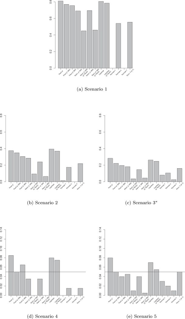
Results for these complex scenarios are displayed graphically for all four test statistics in Figures 3–6. Though there is some variability in the relative performance of the permutation methods across test statistics, we can see that the three fixed g* methods and the two Lagrange methods are nearly always at least as powerful (Scenarios 1–3) as the traditional methods, and are often noticeably more powerful.

Fig. 3.

$\widehat{Q}{(\widehat{A})}_{\mathit{RS}}$ rejection rates (α = 0.05) for complex model simulations. *Results for Scenario 3 based on 198 data sets due to numerical problems.

Fig. 6.

$\widehat{Q}{(\widehat{A})}_Z$ rejection rates (α = 0.05) for complex model simulations. *Results for Scenario 3 based on 198 data sets due to numerical problems.

In terms of type-I error (Scenarios 4 and 5), the traditional methods have a tendency to be overly conservative, whereas the proposed methods tend to be slightly liberal. The Fixed g* (RN), Fixed g* (BN) and Lagrange g* (g* residual) methods seem to have the best type-I error rates among the proposed methods, and are fairly comparable to the traditional methods, with the traditional methods performing best in some cases and the Fixed g* (RN), Fixed g* (BN) and Lagrange g* (g* residual) methods performing best in others.

Among the proposed methods, the Fixed g* (BN), Fixed g* (RN) and Lagrange (g* Residuals) approaches perform best, followed by the Fixed g* and Lagrange g* approaches. The Random g* (RN) and Random g* (BN) methods, also performed reasonably well, but tended to have lower power and very conservative type-I error rates in most cases. The Random g* (RN) (g* residuals) and Random g* (BN) (g* residuals) methods had very low power and extremely conservative type-I error rates in most cases, and performed worst among the proposed methods.

As was the case in the simple linear simulations, it seems as if the Fixed g* (RN), Fixed g* (BN) and Lagrange g* (g* residual) methods are best, as they are generally comparable to the traditional methods in type-I error and, in most cases, noticeably more powerful. Though the Permute X and Permute Y (in T) methods performed fairly well in these complex scenarios, their performance will undoubtedly suffer when larger main effects of the covariates are present, as illustrated in the first two simple linear scenarios when the ad hoc test statistic was used. Given the results of both the simple and complex model simulations, we recommend the use of the Fixed g* (RN), Fixed g* (BN) and Lagrange g* (g* residual) methods in practice.

4 Application to data from a randomized clinical trial

The proposed methods, along with SORA, were applied to data from the Trial of Preventing Hypertension (TROPHY) (Julius et al, 2006). This study included participants with prehypertension, defined as either an average systolic blood pressure of 130 to 139 mm Hg and diastolic blood pressure of no more than 89mm Hg for the three run-in visits (before randomization), or systolic pressure of 139 mm Hg or lower and diastolic pressure between 85 and 89 mm Hg for the three run-in visits. Each subject randomly assigned to receive either two years of candesartan (a hypertension treatment) or placebo, followed by two years of placebo (for all subjects). Subjects had return visits at 1 and 3 months post-randomization, and every 3 months thereafter until month 24. In year 3, clinic visits were at 25 and 27 months, and then every third month thereafter until the end of the study. The study produced analyzable data on 772 subject, with 391 being randomized to candesartan and 381 to placebo. Baseline measurements were age, gender, race (white, black or other), weight, body-mass index (BMI), systolic and diastolic blood pressures, total cholesterol, high density lipoprotein cholesterol (HDL), low density lipoprotein cholesterol (LDL), HDL:LDL ratio, triglycerides, fasting glucose, total insulin, insulin:glucose ratio and creatinine, but the insulin:glucose ratio was dropped from our analysis due to extremely high correlation (≈ 0.98) with total insulin. Additionally, insulin, glucose, HDL, LDL, HDL:LDL ratio and triglycerides were noticeably skewed, so these covariates were log-transformed for the analysis. The endpoint of interest in our analysis is blood pressure (systolic) at 12 months post-randomization. In this study, candesartan has a very obvious beneficial effect on blood pressure, so the question of interest is whether there is a subgroup of patients who should not receive it.

It should be noted that at 12 months post-randomization there was approximately 20% missing data in the outcome due to patient dropout and patients developing hypertension (the endpoint in the original study). Because the endpoint (hypertension) was defined based only on observed blood pressure measurements, missing data due to patients experiencing the event were assumed to be missing at random. There was also a small amount of missingness in the baseline covariates (≤ 4.3%). These missing values were filled in using imputation. All imputation was performed using SAS PROC MI (SAS Institute Inc., Cary, NC). The imputation model included all baseline covariates and all blood pressure measurements up to 12 months post-randomization, stratified by treatment and gender. Because SORA has not been extended to data with missing values, only a single imputation was performed.

As our goal in this case is to identify those individuals who should not receive treatment, the SORA procedure was modified to identify a region in which the treatment effect was zero or negative. The identified region was  ={HDL:LDL ratio < 0.38, HDL cholesterol < 46.02, total insulin ≥25.11} and contained 20 subjects. The estimates $\widehat{Q}{(\widehat{A})}_{\mathit{RS}}$, $\widehat{Q}{(\widehat{A})}_{\mathit{SND}}$, $\widehat{Q}{(\widehat{A})}_{\widehat{g}}$ and $\widehat{Q}{(\widehat{A})}_Z$ had values of −1.63, −8.14, −9.75, and −0.33, respectively. To further assess the identified subgroup, the proposed permutation methods and the four traditional permutation methods were used to obtain p-values for these estimates. For each method, p-values were computed using K = 1000 permutations.

P-values for all test statistics and permutation methods are given in Table 1. As might be expected, given the relative magnitudes of the estimates, $\widehat{Q}{(\widehat{A})}_{\widehat{g}}$ has the smallest p-value for all the methods considered, followed by $\widehat{Q}{(\widehat{A})}_{\mathit{SND}}$, with $\widehat{Q}{(\widehat{A})}_{\mathit{RS}}$ and $\widehat{Q}{(\widehat{A})}_Z$ having the largest p-values. Though nearly always large for $\widehat{Q}{(\widehat{A})}_{\mathit{RS}}$, $\widehat{Q}{(\widehat{A})}_{\mathit{SND}}$, and $\widehat{Q}{(\widehat{A})}_Z$, p-values, including those based on the Fixed g* (RN) and Fixed g* (BN) methods, are fairly small for $\widehat{Q}{(\widehat{A})}_{\widehat{g}}$, an estimate which we have found to perform relatively well in previous work. Thus, though perhaps unlikely, given the results for $\widehat{Q}{(\widehat{A})}_{\mathit{RS}}$, $\widehat{Q}{(\widehat{A})}_{\mathit{SND}}$, and $\widehat{Q}{(\widehat{A})}_Z$, it is possible that there exists a small group of subjects who should not receive candesartan.

Table 1.

P-values for TROPHY data

Method	Estimate
	$\widehat{Q}{(\widehat{A})}_{\mathit{RS}}$	$\widehat{Q}{(\widehat{A})}_{\mathit{SND}}$	$\widehat{Q}{(\widehat{A})}_{\widehat{g}}$	$\widehat{Q}{(\widehat{A})}_Z$
Fixed g*	0.93	0.20	0.05	0.93
Fixed g* (RN)	0.93	0.22	0.05	0.92
Fixed g* (BN)	0.92	0.26	0.05	0.92
Random g* (RN)	0.93	0.27	0.07	0.93
Random g* (RN) (g* residuals)	0.93	0.33	0.11	0.92
Random g* (BN)	0.92	0.28	0.08	0.91
Random g* (BN) (g* residuals)	0.93	0.33	0.11	0.93
Lagrange	0.94	0.34	0.11	0.94
Lagrange (g* residuals)	0.95	0.39	0.14	0.95
Permute y	0.77	0.00	0.00	1.00
Permute X	0.94	0.19	0.05	0.94
Permute T	0.75	0.00	0.00	1.00
Permute y (in T)	0.95	0.19	0.05	0.95

When we permute y or T, the new treatment effect estimates are generally centered around zero, which in this case will most likely lead to a larger “don’t treat” region than that identified using the observed data, for which nearly all treatment effect estimates were positive. These larger “don’t treat” regions for the permuted data will generally have smaller corresponding estimates of Q(Â), which may be why the permute y and permute T approaches give the smallest p-values. However, given the poor performance of these two approaches in our simulations, it may not be wise to trust these methods when testing for interactions, particularly when an ad hoc test statistic is being used.

5 Discussion

We proposed several permutation-based methods which can be used as an alternative to simple permutation test when one wishes to test for interactions. The proposed methods were shown to generally outperform simple permutation tests, particularly when we considered more complex scenarios and test statistics. These methods may help to reduce false positive findings when a pre-defined subgroup identification strategy such as Virtual Twins (Foster et al, 2011) or SORA is employed.

We show in the simple linear model simulations that the fixed g* and Lagrange methods are slightly anti-conservative, and hypothesized that this may be due to the decreased total variance of $y_i^{\ast }$ compared to y_i. Thus, for these methods, it may be helpful to consider inflating the variance of the residuals in step 1 of our algorithm, so that the variance of $y_i^{\ast }$ matches that of y_i. Similarly, the random g* (RN) and random g* (BN) methods were overly conservative in our simple linear model simulations, which we believe is due to an increased total variance of $y_i^{\ast }$ relative to y_i, so for these methods it may be helpful to consider deflating the variance of the residuals in step 1 of our algorithm. We attempted to address these issues by using residuals based on g* (i.e. y − ĥ – g* (T − π)), rather than ĝ for the Lagrange, random g* (RN) and random g* (BN) methods. This was mildly successful for the Lagrange method, but actually worsened the problem for the random g* (RN) and random g* (BN) methods. In the future, it may be interesting to consider other methods of adjusting the variance of the residuals in step 1 of our algorithm.

It may also be interesting to consider additional permutation-based methods. For instance, note that the estimates which result from fitting model (1.1) can be used to obtain estimated responses given treatment and given control (i.e. counterfactuals) for each subject. By fixing the sums of these estimated responses for each individual and permuting the differences (i.e. the treatment effects), we could obtain “null” data in which the overall treatment effect is preserved, but individual treatment effects are removed.

It is worth noting that the permutation methods considered in the paper are, themselves, quite fast. In this manuscript, we focused on the use of these methods with SORA, a systematic subgroup identification procedure which can be very computationally expensive, and as a result, we chose to obtain p-values using K = 100 permutations for our complex model simulations. However, the proposed permutation approaches can be implemented for many different models and test statistics, and the speed with which this can be done depends almost entirely on how much computational time is required to obtain the chosen test statistic. For instance, in our simple linear simulations, obtaining p-values based on K = 1000 permutations sequentially for all 13 methods considered (ignoring the exact test) took only about three minutes for a given data set. In general, we recommend using a large number of permutations (at least 1000, say) when feasible, particularly when the sample size is large. For extremely large sample sizes, one may wish to use considerably more permutations.

Fig. 4.

$\widehat{Q}{(\widehat{A})}_{\mathit{SND}}$ rejection rates (α = 0.05) for complex model simulations. *Results for Scenario 3 based on 198 data sets due to numerical problems.

Fig. 5.

$\widehat{Q}{(\widehat{A})}_{\widehat{g}}$ rejection rates (α = 0.05) for complex model simulations. *Results for Scenario 3 based on 198 data sets due to numerical problems.

References

- Assmann SF, Pocock SJ, Enos LE, Kasten LE. Subgroup analysis and other (mis)uses of baseline data in clinical trials. The Lancet. 2000;355(9209):1064–1069. doi: 10.1016/S0140-6736(00)02039-0. [DOI] [PubMed] [Google Scholar]
- Brookes ST, Whitley E, Peters TJ, Mulheran PA, Egger M, Davey Smith G. Subgroup analyses in randomised controlled trials: quantifying the risks of false-positives and false-negatives. Health technology assessment (Winchester, England) 2001;5(33):1–56. doi: 10.3310/hta5330. [DOI] [PubMed] [Google Scholar]
- Bůžková P, Lumley T, Rice K. Permutation and parametric bootstrap tests for gene-gene and gene-environment interactions. Annals of human genetics. 2011;75(1):36–45. doi: 10.1111/j.1469-1809.2010.00572.x. [DOI] [PMC free article] [PubMed] [Google Scholar]
- Cai T, Tian L, Wong PH, Wei LJ. Analysis of randomized comparative clinical trial data for personalized treatment selections. Biostatistics. 2011;12(2):270–282. doi: 10.1093/biostatistics/kxq060. [DOI] [PMC free article] [PubMed] [Google Scholar]
- Edgington ES. Randomization tests. Marcel Dekker, Inc; New York, NY, USA: 1986. [Google Scholar]
- Foster JC, Taylor JM, Ruberg SJ. Subgroup identification from randomized clinical trial data. Statistics in Medicine. 2011:2867–2880. doi: 10.1002/sim.4322. [DOI] [PMC free article] [PubMed] [Google Scholar]
- Good P. Permutation Tests: A Practical Guide to Resampling Methods for Testing Hypotheses. Springer; 2000. [Google Scholar]
- Julius S, Nesbitt SD, Egan BM, Weber MA, Michelson EL, Kaciroti N, Black HR, Grimm RH, Messerli FH, Oparil S, Schork MA. Feasibility of treating prehypertension with an angiotensin-receptor blocker. New England Journal of Medicine. 2006;354(16):1685–1697. doi: 10.1056/NEJMoa060838. [DOI] [PubMed] [Google Scholar]
- Lipkovich I, Dmitrienko A, Denne J, Enas G. Subgroup identification based on differential effect searcha recursive partitioning method for establishing response to treatment in patient subpopulations. Statistics in Medicine. 2011;30(21):2601–2621. doi: 10.1002/sim.4289. [DOI] [PubMed] [Google Scholar]
- Peto R, Collins R, Gray RN. Large-scale randomized evidence: Large, simple trials and overviews of trials. Journal of Clinical Epidemiology. 1995;48(1):23–40. doi: 10.1016/0895-4356(94)00150-o. [DOI] [PubMed] [Google Scholar]
- Potthoff RF, Peterson BL, George SL. Detecting treatment-by-centre interaction in multi-centre clinical trials. Statistics in Medicine. 2001;20(2):193–213. doi: 10.1002/1097-0258(20010130)20:2<193::aid-sim651>3.0.co;2-#. [DOI] [PubMed] [Google Scholar]
- Ruberg SJ, Chen L, Wang Y. The mean does not mean as much anymore: finding sub-groups for tailored therapeutics. Clinical trials (London, England) 2010;7(5):574–583. doi: 10.1177/1740774510369350. [DOI] [PubMed] [Google Scholar]
- Simon N, Tibshirani R. A permutation approach to testing interactions in many dimensions. 2012 arXiv:1206.6519v1. [Google Scholar]
- Yusuf S, Wittes J, Probstfield J, Tyroler HA. Analysis and interpretation of treatment effects in subgroups of patients in randomized clinical trials. JAMA. 1991;266(1):93–98. [PubMed] [Google Scholar]
- Zhang B, Tsiatis AA, Laber EB, Davidian M. A robust method for estimating optimal treatment regimes. Biometrics. 2012;68(4):1010–1018. doi: 10.1111/j.1541-0420.2012.01763.x. [DOI] [PMC free article] [PubMed] [Google Scholar]