Splice Sites Seldom Slide: Intron Evolution in Oomycetes

Abstract

We examine exon junctions near apparent amino acid insertions and deletions in alignments of orthologous protein-coding genes. In 1,917 ortholog families across nine oomycete genomes, 10–20% of introns are near an alignment gap, indicating at first sight that splice-site displacements are frequent. We designed a robust algorithmic procedure for the delineation of intron-containing homologous regions, and combined it with a parsimony-based reconstruction of intron loss, gain, and splice-site shift events on a phylogeny. The reconstruction implies that 12% of introns underwent an acceptor-site shift, and 10% underwent a donor-site shift. In order to offset gene annotation problems, we amended the procedure with the reannotation of intron boundaries using alignment evidence. The corresponding reconstruction involves much fewer intron gain and splice-site shift events. The frequency of acceptor- and donor-side shifts drops to 4% and 3%, respectively, which are not much different from what one would expect by random codon insertions and deletions. In other words, gaps near exon junctions are mostly artifacts of gene annotation rather than evidence of sliding intron boundaries. Our study underscores the importance of using well-supported gene structure annotations in comparative studies. When transcription evidence is not available, we propose a robust ancestral reconstruction procedure that corrects misannotated intron boundaries using sequence alignments. The results corroborate the view that boundary shifts and complete intron sliding are only accidental in eukaryotic genome evolution and have a negligible impact on protein diversity.

Introduction

Introns disrupt the coding sequence of genes in all known free-living eukaryotes (Rogozin et al. 2012). Key components of the intron-splicing machinery are preserved across great evolutionary distances (Collins and Penny 2005), implying that they are inherited from the last common eukaryotic ancestor (LECA). Intron densities vary widely among taxonomic groups (Jeffares et al. 2006), and comparisons of homologous genes show that their exon–intron structures have diverged in different lineages. Large-scale studies have primarily concentrated on the patterns of intron loss and gain. Intron sequences, aside from the short splicing signals they carry, generally evolve without selective pressure, which makes it necessary to project orthologous gene structures to protein alignments in order to establish intron homology in distant genomes (Rogozin et al. 2005). Various probabilistic methods (Qiu et al. 2004; Carmel et al. 2005; Roy and Gilbert 2005; Csűrös et al. 2008; Csűrös 2008) have served to infer ancestral intron content from presence–absence profiles in conserved alignment regions. Frequently matching exon–intron structures in homologs indicate that about one-third of human introns are inherited from LECA, and that LECA had fairly intron-rich genes (Rogozin et al. 2003; Roy and Gilbert 2005; Carmel et al. 2011; Csűrös et al. 2011).

Gain and loss patterns have been determined routinely using unambiguously aligned sequences (Rogozin et al. 2005; Coulombe-Huntington and Majewski 2007; Csűrös 2008). When one projects the gene structures onto the alignments, it can be observed that in addition to their frequent concurrence in conserved blocks, introns often fall near or opposite to alignment gaps, and thus traditionally excluded from evolutionary reconstruction. Our study precisely aims to deal with sites in hard-to-align coding segments.

Intron boundaries shift if new splice sites spontaneously appear or old ones disappear through genomic point mutations. Splice-site shifts manifest as gaps neighboring exon junctions in the alignment of homologous proteins, just like actual coding insertions and deletions. Such exonization or intronization events create an alternatively spliced isoform that would eventually become the dominant form, possibly after the fixation of compensatory mutations (Lynch 2002; Tarrìo et al. 2008). Indeed, the adoption of intronic segments into the coding sequence and vice versa was posited in vertebrate, fruit fly, and roundworm genomes (Kondrashov and Koonin 2003; Irimia et al. 2008; Farlow et al. 2010), and the exaptation of intronic transposed elements is well-documented (Sorek 2007). It was even suggested that instead of an exogenous source, it is mainly the intronization of coding regions that gave rise to LECA's first spliceosomal introns (Catania and Lynch 2008; Catania et al. 2009). Small-scale genomic changes activating and deactivating splice sites are thus potentially important to the evolution of proteins.

We examine introns near apparent amino acid insertions and deletions in alignments of orthologous protein-coding genes across nine oomycete genomes (see fig. 1). A number of genome projects have targeted important plant pathogens in this group, including Phytophthora ramorum (Tyler et al. 2006), the agent of sudden oak death, and Phytophthora infestans (Haas et al. 2009), the agent of potato blight. Introns in the selected genomes are short and common; see Supplementary Material for statistics. Gene families in oomycetes have dynamic evolutionary histories (Tyler et al. 2006; Seidl et al. 2012) with frequent duplications and losses, reflecting divergent evolutionary pressures. We sought to examine if shifting intron boundaries also contribute to adaptations in this group. In our data set comprising 1,917 ortholog families, 10–20% of introns are near an alignment gap (within 3 amino acids).

Fig. 1.—

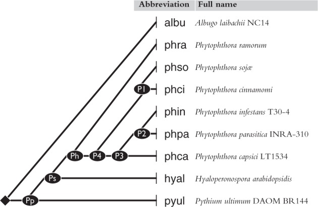
Studied genomes with the phylogeny used in ancestral reconstruction.

We designed a parsimony-based reconstruction of intron loss, gain, and splice-site shift events on a phylogeny, and applied it to the data set. Our initial reconstruction implies that in oomycete lineages, 12% of introns underwent an acceptor-site shift, and 10% underwent a donor-site shift.

A more mundane reason for introns near gaps is that they may be artifacts of genome annotation. Even if contemporary bioinformatics methods are very successful at finding protein-coding genes in DNA sequences, the precise annotation of exon–intron boundaries is extremely difficult, and consequently error-prone (Mathé et al. 2002; Goodswen et al. 2012). Nucleotides close to intron boundaries may resemble genuine splicing signals, and it is not easy to decipher without transcriptional evidence, where the splicing occurs exactly, or if there are alternate splice sites. Excess intron lengths that are multiples of three (3n-introns) attest to the error of gene prediction software annotating complete coding segments as introns (Roy and Penny 2007).

The parsimony reconstruction naturally accommodates the reassignment of exon–intron boundaries using alignment evidence. Using a combined reannotation–reconstruction procedure, the inferred frequency of acceptor- and donor-side shifts drops to 4% and 3%, respectively. These frequencies are not much different from what one would expect by random codon insertions and deletions. In addition to 87 newly proposed introns, the procedure recast more than 900 3n-introns as coding segments, and displaced more than 700 splice sites.

Methods

Data Set

Our data set relies on complete annotated genomes for nine species (see fig. 1) comprising genome sequences with exon–intron structure annotation and translated protein sequences. Genome data were downloaded from the genome portal of the Department of Energy Joint Genome Institute (Nordberg et al. 2014) for Phytophthora capsici (Lamour et al. 2012) and for Phytophthora cinnamomi (Phyca11 and Phyci1 assembly versions, respectively). Data were downloaded from Ensembl Protists (Kersey et al. 2016) for Albugo laibachii (Kemen et al. 2011), P. ramorum and Phytophthora sojae (Tyler et al. 2006), P. infestans (Haas et al. 2009), Hyaloperonospora arabidopsidis (Baxter et al. 2010), and Pythium ultimum (Lévesque et al. 2010) (assembly versions ENA1, ASM14973v1, ASM14975v1, ASM14294v1, HyaAraEmoy2_2.0, and pug). Phytophthora parasitica data come from the Phytophthora parasitica Assembly Dev initiative, Broad Institute (broadinstitute.org), assembly version Ppar329.

Figure 2 illustrates the analysis steps described below.

Fig. 2.—

Outline of the analysis pipeline. 1. Data collection. 2. Conservation in pairwise alignments around the splice sites. 3. Combination of pairwise brackets into intron contexts covering all orthologs. 4. Ancestral reconstruction of splice sites within the contexts.

Ortholog Grouping

We used BLASTP and OrthoMCL (Li et al. 2003) to construct ortholog groups on a total of 162,564 protein sequences. We kept only those families among the 18,955 identified groups that contained exactly one gene for every organism. We removed seven families containing genes that had annotated exon lengths of 0 or 1, resulting in 1,917 ortholog families that were used in the analysis.

Phylogenetic Reconstruction

Protein sequences were aligned within each ortholog group using Muscle (Edgar 2004) with -maxiters 1,000 option for an ample number of refinement iterations. Using GBlocks (Castresana 2000), we selected the 254 most conserved families comprising protein sequences with ≥80% conserved gapless alignment columns, which provided us with 99,962 conserved sites (of which 15,164 were informative ones) for the purposes of phylogenetic reconstruction. RAxML (Stamatakis 2006), when run with different amino-acid substitution models (LG and WAG, Gamma-variation), reported the same maximum-likelihood topology shown in figure 1, and assigned 96–100% bootstrap support to all edges. We note that there is no consensus yet on Phytophthora species phylogeny: Figure 1 agrees with Blair et al. (2008), but differs slightly from Seidl et al. (2012) in the resolution of P. infestans–P. ramorum–P. sojae relationships.

Alignments and Exon Junctions

Annotated exon junctions were projected onto the alignments in a usual manner (Rogozin et al. 2005). Distance to the nearest gap was calculated within extracted pairwise alignments using the following definition. Suppose that in the alignment of genes i, i', a phase 1 or 2 intron interrupts codon k of gene i. If codon k is aligned with a gap in gene i’, then the gap distance is 0. Otherwise, we consider the maximal segment of consecutive matches including k: if it covers codons (k-a), (k-a + 1),…,(k + b), then the upstream gap distance is (a + 1) and the downstream gap distance is (b + 1). The statistical significance for the number of introns opposite a gap (distance 0), or on a match segment boundary (distance 1) was assessed by computing the probability that a codon selected uniformly along all genes included from a genome falls opposite a gap, or exactly on a match segment boundary. The first probability equals D/L, where D codons are deleted from gene i and L is the total coding length; the second probability equals M/(L-D), where M denotes the number of match segments and the denominator respects the condition that the gap distance is at least 1. The P-value for observing a given number of introns at distance 0 (or 1) away from gaps is then calculated as a binomial tail; consult the Supplementary Material for a formal description of the details.

Intron Contexts

Intron contexts are built from conserved codons in pairwise alignments. Conservation is measured by log-odds scores (Durbin et al. 1998) calculated specifically for every genome pair from all the ortholog alignments (see details in Supplementary Material). An anchor is defined as a run of matches within the same match segment, scoring above a predefined threshold τ, without intervening introns in any of the two sequences. In our analysis, threshold τ is chosen as the expected score of four codon matches. We find the nearest upstream and downstream anchors from an exon junction by adapting Kadane's linear-time algorithm for finding a maximum-scoring segment (Bentley 1984). Note that there might be no upstream or downstream anchor: such exon junctions are removed from further consideration.

Intron contexts consist of overlapping regions bracketed by upstream and downstream anchors (see fig. 3A). An intron context provides a consistent coordinate system if the set of its upstream anchors can be placed on a single multidiagonal in the alignment of the underlying genomic sequences, and the same holds for the downstream anchors.

Fig. 3.—

Intron context example. (A) Conservation in pairwise alignments provide anchors for the intron site. Vertical bars mark where phase-0 introns are spliced out from the phra and phci sequences. Upstream and downstream anchors formed by high-scoring segment pairs are shown by horizontal shading along the sequences. (B) Transferring splice site annotation from one sequence to another within the intron context. Horizontal (green) shading demarcates introns. The coding alignment implies a deletion in the phin and phca sequences, and a large insertion in the albu sequence. There is, however, an annotated acceptor site in phpa (as well as in pyul, hyal, phra, and phso, not shown here), which yields alternative intron boundaries for phin and phca, as projected from the 3' end of the context. Same holds for albu, which also has a possible donor site found by projecting from the 5' end.

Reannotation and Ancestral Inference

Given a consistent intron context, genomic coordinates of splice site along one sequence are projected onto another using the diagonal defined by the anchors. More precisely, we project the two intronic positions immediately next to the splice site using upstream diagonals for donor, and downstream diagonals for acceptor sites, and we inspect the 2-nt genomic sequence motif found there. Candidate donor motifs are GT, GC, AT, and candidate acceptor motifs are AG, AC, TG. Candidate introns are formed by pairing sites with adequate motifs in all (annotated and projected) donor–acceptor combinations provided they are in matching phases, do not introduce premature stop codons, and contain a minimum of 24 nucleotides.

Given a phylogeny, we label every tree node either with pairs of donor–acceptor site coordinates (d, a), or with Ø for no intron. Labels are encoded using donor-side and acceptor-side coordinate projections onto the same (arbitrary) reference gene. A terminal node with an annotated intron can be considered for Ø only if the intron length is a multiple of three, and the exonified sequence introduces no in-frame stop codon. For ancestral nodes, we consider the label set comprising all phase-matched pairs formed by donor and acceptor sites at the terminal nodes, and Ø. At terminal nodes, the displacement of either splice site, or the exonification of a complete intron (label Ø) is counted with unit penalty. The reconstruction uses the following edge penalties (which were chosen so that two losses are favored over one gain, and up to five splice sites can be reannotated for the price of a loss or a shift): loss = 5, gain = 12, donor-side shift = 5, acceptor-side shift = 5, intron sliding = 10. The score for a complete labeling is the sum of edge penalties, plus the reannotation penalties at terminal nodes. A minimum-score labeling is found by adapting Sankoff's dynamic programming algorithm (Sankoff and Rousseau 1975) for the context-specific label set. When reannotations are not allowed, we use the same reconstruction algorithm with reannotation penalty set to ∞.

Software Availability

The developed analysis method was implemented as a standalone Java package. The source code and the JAR archive along with the data set can be downloaded from http://github.com/csurosm/ReSplicer.

Results

We investigate the gene structures in nine oomycete genomes, including six Phytophthora species (capsici, cinnamomi, infestans, parasitica, ramorum, sojae), P. ultimum, H. arabidopsidis, and A. laibachii. First, we examine intron length distributions in the selected genomes, then compare where the splice sites fall with respect to multiple alignments of orthologous genes.

Intron Length Distributions Indicate Widespread Misannotation

We computed the distribution of intron lengths across all annotated genes within every genome. The distributions reveal both organism-specific idiosyncrasies and annotation artifacts.

Figure 4 shows the example of P. ramorum. First, the distribution appears to be a mixture of a sharply concentrated Poisson-like peak around the typical intron length, and a geometric distribution. The latter is presumably influenced by the gene finding software. Namely, common probabilistic models include a Markov state for intronic segments (Mathé et al. 2002), for which the duration length is geometrically distributed, and length j thus occurs with prior probability proportional to p (1-p) ^j-1 for some state-transition parameter p. The geometric prior is manifest in very short annotated introns, as well as in the slowly decaying tail with long introns (points scattered around a straight line on a semi-log graph).

Fig. 4.—

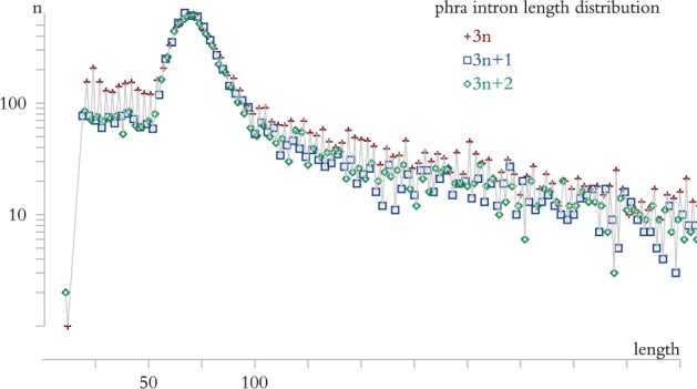
Distribution of annotated intron lengths in P. ramorum. Note the excess of 3n-length introns, and the geometrically decaying tail after the typical 50–100-nt intron length.

Second, intron lengths that are exact multiples of three occur more often than (3n + 1) and (3n + 2) intron lengths. Roy and Penny (2007) attributed the excess of 3n-introns to errors of gene prediction, annotating exonic sequences as introns. In our case, five genome annotations suffer from the same problem (see Supplementary Material), in all likelihood those that were completed without sufficient transcription data (EST or RNA-Seq). Indeed, introns of P. parasitica, which were annotated relying on copious transcription data, exhibit neither an excess of 3n-lengths, nor a pronounced geometric tail.

Annotated Introns Often Coincide with Deletions or Insertions

We selected the set of 1,917 protein-coding gene families with exactly one homolog in each genome, and computed a multiple alignment of amino acid sequences for each. Following a standard pipeline for the analysis of gene structure evolution (Rogozin et al. 2005), we projected the gene structures onto the alignments. Introns may interrupt codons after the first or second nucleotide (phase-1 and phase-2 introns), or may fall between codons (phase-0). The displacement of the splice sites for an otherwise conserved intron entails the inactivation or activation of coding nucleotides next to the boundary, yielding alignment gaps. Similarly, coding alignment gaps result from the intronization of a region (simultaneous activation of donor and acceptor sites), or the exonization of an entire intron (simultaneous deactivation of splice sites). Conceivably, some genomic recombination events may also correspond to intron loss and gain also accompanied with coding indels at the intron boundaries.

We found that for most of our studied genomes, the projected placement of exon boundaries is not random with respect to coding alignment gaps. Table 1 shows that P. ramorum and P. infestans exon junctions align with gaps or are within one codon away from a gap much more often than what would be expected from a uniformly random placement. (See the Supplementary Material for all genome pairs.) For example, 102 phase-1 introns in P. ramorum fall into a codon right after a gap when only about 8 should.

Table 1.

Gaps near introns

	n	Aligned with gap			5′ss -1aa			3′ss +1aa
		obs.	exp.	P-value	obs.	exp.	P-value	obs.	exp.	P-value
Phase 1
phra	1,002	134	56.4	5 × 10−20	102	8.4	4 × 10−74	62	8.4	4 × 10−33
phin	971	98	41.8	2 × 10−14	103	8.4	3 × 10−75	55	8.4	5 × 10−27
Phase 2
phra	1,012	110	57.0	7 × 10−11	36	8.8	3 × 10−12	101	8.8	3 × 10−71
phin	976	89	42.0	6 × 10−11	33	8.6	1 × 10−10	94	8.6	2 × 10−64

Note.—Statistics are shown for P. ramorum–P. sojae (phra row) and P. infestans–P. cinnamomi (phin row) pairwise alignments. After projecting all introns (column n) onto the aligned protein sequences, we searched for the nearest insertions or deletions both upstream and downstream. 5'ss-1aa and 3'ss + 1aa indicate that the intron-containing codon is next to a gap upstream and downstream, respectively. Observed (obs.) counts are typically much larger than what would be expected (exp.) under the null model of random intron placement with respect to a fixed alignment, which was used to define the P-values. (Note that the expected values upstream and downstream are the same for ±1aa.).

Ancestral Reconstruction Suggests Rampant Splice-Site Displacement

Notwithstanding misannotation problems, the extent to which bona fide remodeling of the splice sites contributed to genome evolution can be assessed in a phylogenetic context. We devised a novel analysis protocol to determine site homologies, and to place splice-site mutations on an evolutionary tree. Our procedure relies on bracketing an intron-bearing portion of the alignment by anchors of conserved segments. An anchor is defined as the closest (upstream or downstream) run of conserved alignment columns between two sequences within the multiple alignment: both sequences must have matching codons or matching gaps in each column, and no introns. Conservation is measured by log-odds scoring (Durbin et al. 1998) of codons, specific to the genome pair. Splice-site coordinates are then encoded as offsets from the anchors, which lets us decide the homologies between genomic positions in different sequences. After finding the closest anchors upstream and downstream for an intron in a sequence with respect to all other sequences, the pairwise bracketed regions are combined into intron contexts (see fig. 3B.)

Consider the diagonal (in the edit graph) for an anchor matching genomic positions (i,j), (i + 1, j + 1), (i + 2,j + 2), … between two coding sequences (for simplicity, assume that all transcripts are on the forward strand). The corresponding diagonal offset Δ = (j-i) defines how positions should be projected from the first sequence to another. A set of anchors provides a consistent coordinate system for projecting coordinates from any sequence to any other, if for every sequence triple A, B, C with diagonal offsets Δ(A→B), Δ(B→C), Δ(A→C), transitivity holds: Δ(A→C)= Δ(A→B)+Δ(B→C). (Equivalently, the anchors are on the same multidiagonal in the alignment of the genomes.) We thus kept the intron contexts where every sequence had at most one intron, and both the set of upstream and downstream anchors provided consistent coordinate systems. The resulting data set, which is used as input for ancestral reconstruction, contains 4,376 such contexts, of which 1,618 have introns in only a single genome.

We computed a phylogeny for the nine organisms with RAxML (Stamatakis 2006) from highly conserved ortholog sequences. Figure 1 shows the most likely tree found by the software. (Other trees with slightly different relationships among Phytophthora species gave similar results.)

In order to reconstruct the history of splice sites within an intron context, we adapted Sankoff's dynamic programming (Sankoff and Rousseau 1975), which computes the parsimony labeling for nodes of a phylogeny under arbitrary penalties. (Loss and each site shift is penalized by 5, and intron gain is penalized by 12 on every edge.)

Table 2 shows the result of the ancestral reconstruction. Excluding contexts with unique introns specific to a single genome, 340 of the 2,758 remaining histories involve at least one acceptor site shift, and 280 involve at least one donor site shift (43 contexts have both); see Supplementary Material for Venn diagrams. In other words, according to the ancestral inference, more than one-fifth of non-unique introns underwent some boundary change at least once during oomycete evolution.

Table 2.

Ancestral inference without reannotated splice sites

Branch		Unique	Intron			5′ (donor) shift		3′ (acceptor) shift
Child	Parent	Intron	Loss	Gain	Conservation	←(I)	→(E)	←(E)	→(I)
albu	root	569	224	0	2,253	19	20	20	29
phra	Ph	140	42	35	1,711	19	36	16	45
phso	P1	121	34	30	1,718	12	29	13	32
phci	P1	40	31	37	1,743	3	16	7	7
P1	P4		39	8	1,893	0	1	1	1
phin	P2	228	13	60	1,753	13	28	9	26
phpa	P2	4	45	1	1,798	2	1	3	1
P2	P3		19	1	1,877	1	0	2	0
phca	P3	216	35	40	1,625	12	16	10	29
P3	P4		61	25	1,868	1	3	1	4
P4	Ph		32	9	1,921	3	1	1	1
Ph	Ps		44	8	1,940	1	2	5	2
hyal	Ps	40	109	3	1,313	28	30	30	105
Ps	Pp		621	0	1,975	4	1	7	8
pyul	Pp	260	154	0	2,291	21	31	22	34
Pp	root		5	0	2,586	6	9	6	11
Total		1,618	1,508	257	2,620a	145	224	153	335

^aIn the last row, the conservation entry is the number of introns present at the root.

(E) = exonization, (I) = intronization. Intron conservation means that the splice sites did not shift. Evolutionary events (starting with the loss column) are counted only for non-unique introns.

Combining Ancestral Reconstruction with Sequence Homology Yields Plausible Splice Sites and Suggests That Intron Boundaries Shift Only Rarely

The simplest reason for splice sites coinciding with gaps is that boundaries are annotated erroneously. The misannotation hypothesis is corroborated by the intron length distributions. Our ancestral reconstruction framework accommodates a more nuanced analysis, in which misannotated splice sites can be taken into consideration, as annotations can be transferred from one sequence to another within an intron context. For every pair of annotated splice sites, we examine the genomic sequence in every other sequence at the projected positions, and if they yield plausible unannotated splicing motifs, we record them as candidate sites. See figure 3B for an illustration. In addition, for every 3n-length intron, we add a candidate absence annotation, if such a change does not introduce a stop codon. The plausibility of splicing at a projected 5' or 3' site is further judged solely on the basis of the intronic dinucleotide motif on the boundary. Taking into account the surprising diversity of non-canonical splicing motifs (Jackson 1991; Hall and Padgett 1994; Szafranski et al. 2007; Parada et al. 2014), we allow the most frequent dinucleotides in addition to the canonical GT.AG splicing motifs (GC and AT on the donor side, AC and TG on the acceptor side).

Within a context, we consider thus all candidate labelings at the terminal nodes: original annotations, introns using the projected splice sites (while paying attention to proper phasing), and discounted 3n-length introns. Including a penalty for labeling a terminal node with reannotated splice sites is straightforward in the parsimony framework. We imposed a reannotation cost of 1, and performed the ancestral reconstruction using otherwise the same penalties as before.

Reannotations can be of four kinds: exonification of an annotated intron, intronification of an annotated coding segment, and displacement of donor or acceptor sites. Table 3 shows the number of updated annotations per genome. Phytophthora parasitica (phpa) stands out in quality, as our procedure introduces only a handful of changes. The other four Phytophthora genome annotations have plenty of suspect 3n-introns: hundreds of them can be exonified, as they contain no stop codons, and homologs have matching splice sites. In the A. laibachii and H. arabidopsidis genomes, missed introns are more common than eagerly annotated ones, hinting at a conservative annotation procedure. In general, introns are detected in the genome sequences, but their boundaries may need correction—slightly more often on the 3' than on the 5' end. The large majority of corrected splice patterns use the canonical GT.AG splicing motif, but the algorithm uncovers putative non-canonical motifs by the transferred annotations (Table 3), in general agreement with the confirmed presence of non-canonical splice sites in humans (Parada et al. 2014) and P. sojae (Shen et al. 2011).

Table 3.

Reannotated intron boundaries

Genome	Exonified	Intronified	Displaced donor	Displaced acceptor
albu	14	21	26	24
phca	193	1	22	26
phci	75	8	20	17
phin	285	4	36	34
phpa	2	1	4	10
phra	162	8	54	54
phso	148	7	37	46
pyul	22	5	42	44
Total	925	87	285	369

Intron motif	GT.AG	GC.AG	GT.TG	GT.AC	AT.AG
Newly proposed	593 (80%)	72(9.7%)	39 (5.3%)	19 (2.6%)	13 (1.8%)
Human frequency	98.9827%	0.8890%	0.0180%	0	0.0117%

Note.—On top: newly introduced annotations by genome. On bottom: frequency of the top 5 intron motifs in intronified coding sequences and displaced intron boundaries. Intron motif frequencies in human are taken from Parada et al. (2014).

Table 4 tallies the context histories, and shows that there are notably fewer evolutionary changes implied after the reannotations. The number of introns unique to a single genome decreases substantially (1,005 instead of 1,618), as 3 out of 8 are 3n-length without in-frame stop codons. Conversely, non-unique introns have fewer events in their histories. Most remarkably, the inference implies much fewer intron gains (13 instead of 257).

Table 4.

Ancestral inference with reannotated splice sites

Branch		Unique	Intron			5′ (donor) shift		3′ (acceptor) shift
Child	Parent	Intron	Loss	Gain	Conservation	←(I)	→(E)	←(E)	→(I)
albu	root	556	201	0	2,312	11	8	9	17
phra	Ph	22	35	1	1,799	4	1	2	5
phso	P1	14	18	1	1,784	1	0	1	1
phci	P1	18	17	0	1,762	0	1	0	1
P1	P4		39	3	1,878	0	0	2	0
phin	P2	40	11	0	1,771	5	0	2	4
phpa	P2	2	9	0	1,804	0	1	0	0
P2	P3		16	1	1,843	1	0	0	1
phca	P3	93	33	4	1,632	5	1	0	11
P3	P4		59	1	1,858	0	1	1	0
P4	Ph		30	0	1,914	1	1	1	2
Ph	Ps		44	1	1,942	2	1	2	1
hyal	Ps	19	76	1	1,478	8	6	10	15
Ps	Pp		620	0	1,982	1	0	4	5
pyul	Pp	241	150	0	2,356	6	11	8	11
Pp	root		4	0	2,593	3	7	5	7
Total		1,005	1,362	13	2,616a	48	39	47	81

^aIn the last row, the conservation entry is the number of introns present at the root.

(E) = exonization, (I) = Intronization. Intron conservation means that the splice sites did not shift. Evolutionary events (starting with the loss column) are counted only for non-unique introns.

Splice-site shifts also become less common. Whereas the original annotations imply a total of 857 shift events, only about a quarter of them remain after the reannotations. Looking at it from another angle, 452 original intron contexts have a history involving at least one shift event, but only 149 of them do after the reannotations (see Supplementary Material).

Our definition of intron context does not restrict the extent of site shifts explicitly. There is, however, an implicit constraint due to selecting the nearest conserved regions in the anchoring procedure. Figure 5 plots the distribution of intron boundary displacements. Shorter displacements are more frequent than longer ones, and the overwhelming majority of shift distances are multiples of three, which is not surprising, as otherwise the change would be accompanied with a frameshift in all downstream codons (Lynch 2002). For the 5' intron boundary, shifts are about equally likely toward the exonic and the intronic side, (30–30 are of length at most 15 nucleotides). Displacements on the 3' side are somewhat more frequent than on the 5', and tend to favor the downstream direction (upstream, and downstream, 41 vs. 51 are within 15 nt).

Fig. 5.—

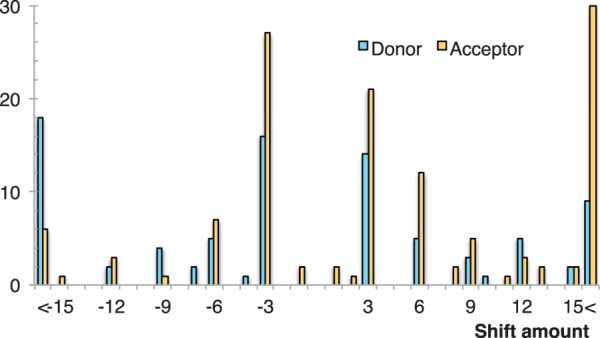
Shifting intron boundaries. Y axis plots the number of shifts summed across all lineages on the 5' (donor) and 3' (acceptor) sides. X axis is the extent of the displacement in nucleotides; positive numbers correspond to transcrip0074 direction. The bars on the two extremes (“<”) tally all shifts less than -15 nt and more than 15 nt, respectively.

Discussion

The evolutionary relevance of spliceosomal introns has been pondered and investigated ever since the discovery of the disjointedness of eukaryotic genes (Gilbert 1978). Some early reports about the coincidence of exon junctions and protein domain boundaries (Craik et al. 1983; de Souza et al. 1997; Sato et al. 1999) gave support to an “introns-early” theory of origins; namely, that introns predate the split of the eukaryotic domain, and are rather an ancestral feature of gaps between functioning mini-genes that correspond to protein domains. In this context, sliding intron boundaries provide a means to adjust protein surface features formed by the peptide sequence at exon junctions (Craik et al. 1983; Kondrashov and Koonin 2003). Intron sliding can be conceptualized as a two-step process of compensatory shifts on the donor and acceptor side, where the allele introduced by the first shift can stay silent via nonsense-mediated decay until the second shift is acquired (Lynch 2002). The resulting coding sequence exhibits no indels with respect to the ancestor. Widespread intron sliding could account for the diversity of intron positions in eukaryotic lineages. Beyond the anecdotal cases, however, extensive data sets of homologous gene alignments cast doubt on a “strong” intron sliding theory (Stoltzfus et al. 1997; Rogozin et al. 2000): it seems that gene structure diversity results from the gain and loss of complete introns.

Intron gain and loss patterns have been scrutinized exhaustively using whole genomes (Rogozin et al. 2003; Yandell et al. 2006; Coulombe-Huntington and Majewski 2007; Stajich et al. 2007; Carmel et al. 2011; Csűrös et al. 2011). The present study aims to quantify boundary sliding comprehensively, dealing with mutations neglected in intron gain–loss inferences. We know of only two in-depth investigations addressing intron sliding in entire evolutionary clades: Roy (2009) looked at four complete Cryptococcus genomes, and Lehmann et al. (2010) examined 31 Drosophila genomes. Both found only a handful of examples for boundary shifts. Our study targets oomycete genomes, which have predominantly short, but not too infrequent introns, making the analysis of exon–intron sequences convenient and fairly reliable. We introduce a novel, robust algorithm for reconstructing intron gain, loss, and shift events in a phylogenetic context. At first sight, the data set implies that splice-site shifts occurred frequently in oomycete evolution given the often mismatched boundaries of overlapping introns in gene alignments. In contrast with the data of Roy (2009) and Lehmann et al. (2010), our gene annotations do not have strong support from transcriptional evidence, and the ancestral reconstruction is suspect to be confounded by annotation errors. We show that incorporating a splice-site reannotation procedure into the ancestral reconstruction algorithm provides a remedy. After suggesting 1,666 reannotated boundaries in our data set of 4,376 aligned intron sites, the reconstructed histories involve much fewer intron gain and splice-site shift events—respectively, 13 instead of 257 and 215 instead of 857, see Tables 2 and 4. In particular, three out of four apparent boundary shifts can be explained instead by an alternative plausible splice site that went unannotated but aligns well with exon junctions in homologs. We have not attempted to resolve whether they correspond to splicing isoforms (alternative or dominant), but the lack of inferred shifts in genome annotations supported by transcription evidence, as in the case of P. parasitica, suggests that shifts are indeed very rare, and are not more common than coding indels occurring near exon junctions by happenstance.

Our study underscores the importance of using curated gene structure annotations in comparative studies. When other evidence is not available, we propose a robust ancestral reconstruction procedure that corrects misannotated intron boundaries using sequence alignments. We applied the reconstruction to a comprehensive data set over poorly annotated genomes. Our results corroborate the view that boundary shifts and complete intron sliding are only accidental in eukaryotic genome evolution and have a negligible impact on protein diversity.

Supplementary Material

Supplementary Material is available at Genome Biology and Evolution online (http://www.gbe.oxfordjournals.org/).

Literature Cited

- Bentley J. 1984. Programming pearls: algorithm design techniques. Comm. ACM 27:865–873. [Google Scholar]
- Baxter L, et al. 2010. Signatures of adaptation to obligate biotrophy in the Hyaloperonospora arabidopsidis genome. Science 330:1549–1551. [DOI] [PMC free article] [PubMed] [Google Scholar]
- Blair JE, Coffey MD, Park SY, Geiser DM, Kang S. 2008. A multi-locus phylogeny for Phytophthora utilizing markers derived from complete genome sequences. Fung. Genet. Biol. 45:266–277. [DOI] [PubMed] [Google Scholar]
- Carmel L, Rogozin IB, Wolf YI, Koonin EV. 2005. An expectation-maximization algorithm for analysis of evolution of exon-intron structure of eukaryotic genes. Lect. Notes Comput. Sci. 3678:35–46. [Google Scholar]
- Carmel L, Rogozin IB, Wolf YI, Koonin EV. 2011. Patterns of intron gain and conservation in eukaryotic genes. BMC Evol. Biol. 7:192.. [DOI] [PMC free article] [PubMed] [Google Scholar]
- Castresana J. 2000. Selection of conserved blocks from multiple alignments for their use in phylogenetic analysis. Mol. Biol. Evol. 17:540–552. [DOI] [PubMed] [Google Scholar]
- Catania F, Lynch M. 2008. Where do introns come from? PLoS ONE 6:e283.. [DOI] [PMC free article] [PubMed] [Google Scholar]
- Catania F, Gao X, Scofield DG. 2009. Endogenous mechanisms for the origins of spliceosomal introns. J. Hered. 100:591–596. [DOI] [PMC free article] [PubMed] [Google Scholar]
- Collins L, Penny D. 2005. Complex spliceosomal organization ancestral to extant eukaryotes. Mol. Biol. Evol. 22:1053–1066. [DOI] [PubMed] [Google Scholar]
- Coulombe-Huntington J, Majewski J. 2007. Characterization of intron loss events in mammals. Genome Res. 17:23–32. [DOI] [PMC free article] [PubMed] [Google Scholar]
- Craik CS, Rutter WJ, Fletterick R. 1983. Splice junctions: associations with variation in protein structure. Science 220:1125–1129. [DOI] [PubMed] [Google Scholar]
- Csűrös M, Rogozin IB, Koonin EV. 2008. Extremely intron-rich genes in the alveolate ancestors inferred with a flexible maximum likelihood approach. Mol. Biol. Evol. 25:903–911. [DOI] [PubMed] [Google Scholar]
- Csűrös M, Rogozin IB, Koonin EV. 2011. A detailed history of intron-rich eukaryotic ancestors inferred from a global survey of 100 complete genomes. PLoS Comput. Biol. 7:e1002150.. [DOI] [PMC free article] [PubMed] [Google Scholar]
- Csűrös M. 2008. Malin: maximum likelihood analysis of intron evolution in eukaryotes. Bioinformatics 24:1538–1539. [DOI] [PMC free article] [PubMed] [Google Scholar]
- Durbin R, Eddy SR, Krogh A, Mitchison G. 1998. Biological Sequence analysis: probabilistic models of proteins and nucleic acids. Cambridge: Cambridge University Press. [Google Scholar]
- Edgar RC. 2004. MUSCLE: multiple sequence alignment with high accuracy and high throughput. Nucleic Acids Res. 32:1792–1797. [DOI] [PMC free article] [PubMed] [Google Scholar]
- Farlow A, Meduri E, Dolezal M, Hua L, Schlötterer C. 2010. Nonsense-mediated decay enables intron gain in Drosophila. PLoS Genet. 6:e1000819.. [DOI] [PMC free article] [PubMed] [Google Scholar]
- Gilbert W. 1978. Why genes in pieces? Nature 271:501.. [DOI] [PubMed] [Google Scholar]
- Goodswen SJ, Kennedy PJ, Ellis JT. 2012. Evaluating high-throughput ab initio gene finders to discover proteins encoded in eukaryotic pathogen genomes missed by laboratory techniques. PLoS ONE 7:e50609.. [DOI] [PMC free article] [PubMed] [Google Scholar]
- Haas BJ, Kamoun S, et al. 2009. Genome sequence and analysis of the Irish potato famine pathogen Phytophthora infestans. Nature 461:393–398. [DOI] [PubMed] [Google Scholar]
- Hall SL, Padgett RA. 1994. Conserved sequences in a class of rare eukaryotic nuclear introns with non-consensus splice sites. J. Mol. Biol. 239:357–365. [DOI] [PubMed] [Google Scholar]
- Irimia M, et al. 2008. Origin of introns by `intronization' of exonic sequence. Trends Genet. 24:378–381. [DOI] [PubMed] [Google Scholar]
- Jackson IJ. 1991. A reappraisal of non-consensus mRNA splice sites. Nucleic Acids Res. 19:3795–3798. [DOI] [PMC free article] [PubMed] [Google Scholar]
- Jeffares DC, Mourier T, Penny D. 2006. The biology of intron gain and loss. Trends Genet. 22:16–22. [DOI] [PubMed] [Google Scholar]
- Kemen E, et al. 2011. Gene gain and loss during evolution of obligate parasitism in the white rust pathogen of Arabidopsis thaliana. PLoS Biol. 9:e1001094.. [DOI] [PMC free article] [PubMed] [Google Scholar]
- Kersey PJ, et al. 2016. Ensembl Genomes 2016: more genomes, more complexity. Nucleic Acids Res. 44:D574–D580. [DOI] [PMC free article] [PubMed] [Google Scholar]
- Kondrashov FA, Koonin EV. 2003. Evolution of alternative splicing: deletions, insertions and origin of functional parts of proteins from intron sequences. Trends Genet. 19:115–119. [DOI] [PubMed] [Google Scholar]
- Lamour KH, et al. 2012. Genome sequencing and mapping reveal loss of heterozygosity as a mechanism for rapid adaptation in the vegetable pathogen Phytophthora capsici. Mol. Plant Microbe. Interact. 25:1350–1360. [DOI] [PMC free article] [PubMed] [Google Scholar]
- Lehmann J, Eisenhardt C, Stadler PF, Krauss V. 2010. Some novel intron positions in conserved drosophila genes are caused by intron sliding or tandem duplication. BMC Evol. Biol. 10:156.. [DOI] [PMC free article] [PubMed] [Google Scholar]
- Lévesque CA, et al. 2010. Genome sequence of the necrotrophic plant pathogen Pythium ultimum reveals original pathogenicity mechanisms and effector repertoire. Genome Biol. 11:R73.. [DOI] [PMC free article] [PubMed] [Google Scholar]
- Li L, Stoeckert CJ, Roos DS. 2003. OrthoMCL: identification of ortholog groups for eukaryotic genomes. Genome Res. 13:2178–2189. [DOI] [PMC free article] [PubMed] [Google Scholar]
- Lynch M. 2002. Intron evolution as a population-genetic process. Proc. Natl. Acad. Sci. U S A. 99:6118–6123. [DOI] [PMC free article] [PubMed] [Google Scholar]
- Mathé C, Sagot MF, Schiex T, Rouzé P. 2002. Current methods of gene prediction, their strengths and weaknesses. Nucleic Acids Res. 30:4103–4117. [DOI] [PMC free article] [PubMed] [Google Scholar]
- Nordberg H, et al. 2014. The genome portal of the Department of Energy Joint Genome Institute: 2014 updates. Nucleic Acids Res. 42:D26–D31. [DOI] [PMC free article] [PubMed] [Google Scholar]
- Parada GE, Munita R, Cerda CA, Gysling K. 2014. A comprehensive survey of non-canonical splice sites in the human transcriptome. Nucleic Acids Res. 42:10564–10578. [DOI] [PMC free article] [PubMed] [Google Scholar]
- Qiu WG, Schisler N, Stoltzfus A. 2004. The evolutionary gain of spliceosomal introns: sequence and phase preferences. Mol. Biol. Evol. 21:1252–1263. [DOI] [PubMed] [Google Scholar]
- Rogozin IB, Lyons-Weiler J, Koonin EV. 2000. Intron sliding in conserved gene families. Trends Genet. 16:430–432. [DOI] [PubMed] [Google Scholar]
- Rogozin IB, Wolf YI, Sorokin AV, Mirkin BG, Koonin EV. 2003. Remarkable interkingdom conservation of intron positions and massive, lineage-specific intron loss and gain in eukaryotic evolution. Curr. Biol. 13:1512–1517. [DOI] [PubMed] [Google Scholar]
- Rogozin IB, Sverdlov AV, Babenko VN, Koonin EV. 2005. Analysis of evolution of exon-intron structure of eukaryotic genes. Brief. Bioinform. 6:118–134. [DOI] [PubMed] [Google Scholar]
- Rogozin IB, Carmel L, Csűrös M, Koonin EV. 2012. Origin and evolution of spliceosomal introns. Biol. Direct. 7:11.. [DOI] [PMC free article] [PubMed] [Google Scholar]
- Roy SW. 2009. Intronization, de-intronization and intron sliding are rare in Cryptococcus. BMC Evol. Biol. 9:192.. [DOI] [PMC free article] [PubMed] [Google Scholar]
- Roy SW, Gilbert W. 2005. Complex early genes. Proc. Natl. Acad. Sci. U S A. 102:1986–1991. [DOI] [PMC free article] [PubMed] [Google Scholar]
- Roy SW, Penny D. 2007. Intron length distributions and gene prediction. Nucleic Acids Res. 35:4737–4742. [DOI] [PMC free article] [PubMed] [Google Scholar]
- Sankoff D, Rousseau P. 1975. Locating the vertices of a Steiner tree in arbitrary metric space. Math Programm. 9:240–246. [Google Scholar]
- Sato Y, Niimura Y, Yura K, Go M. 1999. Module–intron correlation and intron sliding in family F/10 xylanase genes. Gene 238:99–101. [DOI] [PubMed] [Google Scholar]
- Seidl MF, Van den Ackerveken G, Govers F, Snel B. 2012. Reconstruction of oomycete genome evolution identifies differences in evolutionary trajectories leading to present-day large families. Genome Biol. Evol. 4:199–211. [DOI] [PMC free article] [PubMed] [Google Scholar]
- Shen D, Ye W, Dong S, Wang Y, Dou D. 2011. Characterization of intronic structures and alternative splicing in Phytophthora sojae by comparative analysis of expressed sequence tags and genomic sequences. Can. J. Microbiol. 57:84–90. [DOI] [PubMed] [Google Scholar]
- Sorek R. 2007. The birth of new exons: mechanisms and evolutionary consequences. RNA 13:1603–1608. [DOI] [PMC free article] [PubMed] [Google Scholar]
- de Souza SJ, Long M, Schoenbach L, Roy SW, Gilbert W. 1997. The correlation between introns and the three-dimensional structure of proteins. Trends Genet. 205:41–44. [DOI] [PubMed] [Google Scholar]
- Stajich JE, Dietrich FS, Roy SW. 2007. Comparative genomic analysis of fungal genomes reveals intron-rich ancestors. Genome Biol. 8:R223.. [DOI] [PMC free article] [PubMed] [Google Scholar]
- Stamatakis A. 2006. RAxML-VI-HPC: maximum likelihood-based phylogenetic analyses with thousands of taxa and mixed models. Bioinformatics 22:2688–2690. [DOI] [PubMed] [Google Scholar]
- Stoltzfus A, Longsdon JM, Palmer JD, Doolittle WF. 1997. Intron “sliding” and the diversity of intron positions. Proc. Natl. Acad. Sci. U S A. 94:10739–10744. [DOI] [PMC free article] [PubMed] [Google Scholar]
- Szafranski K, et al. 2007. Violating the splicing rules: TG dinucleotides function as alternative 3' splice sites in U2-dependent introns. Genome Biol. 8:R154.. [DOI] [PMC free article] [PubMed] [Google Scholar]
- Tarrìo R, Ayala FJ, Rodríguez-Trelles F. 2008. Alternative splicing: a missing piece in the puzzle of intron gain. Proc. Natl. Acad. Sci. U S A. 105:7223–7228. [DOI] [PMC free article] [PubMed] [Google Scholar]
- Tyler BM, et al. 2006. Phytophthora genome sequences uncover evolutionary origins and mechanisms of pathogenesis. Science 313:1261–1266. [DOI] [PubMed] [Google Scholar]
- Yandell M, et al. 2006. Large-scale trends in the evolution of gene structures within 11 animal genomes. PLoS Comput. Biol. 2:e15. [DOI] [PMC free article] [PubMed] [Google Scholar]
Associated Data
This section collects any data citations, data availability statements, or supplementary materials included in this article.