Multiscale analysis of neurite orientation and spatial organization in neuronal images

Abstract

The spatial organization of neurites, the thin processes (i.e., dendrites and axons) that stem from a neuron's soma, conveys structural information required for proper brain function. The alignment, direction and overall geometry of neurites in the brain are subject to continuous remodeling in response to healthy and noxious stimuli. In the developing brain, during neurogenesis or in neuroregeneration, these structural changes are indicators of the ability of neurons to establish axon-to-dendrite connections that can ultimately develop into functional synapses. Enabling a proper quantification of this structural remodeling would facilitate the identification of new phenotypic criteria to classify developmental stages and further our understanding of brain function. However, adequate algorithms to accurately and reliably quantify neurite orientation and alignment are still lacking. To fill this gap, we introduce a novel algorithm that relies on multiscale directional filters designed to measure local neurites orientation over multiple scales. This innovative approach allows us to discriminate the physical orientation of neurites from finer scale phenomena associated with local irregularities and noise. Building on this multiscale framework, we also introduce a notion of alignment score that we apply to quantify the degree of spatial organization of neurites in tissue and cultured neurons. Numerical codes were implemented in Python and released open source and freely available to the scientific community.

1 Introduction

Estimating neurite orientation and quantifying their spatial organization are highly relevant in many areas of neuroscience research associated with neuronal development, such as neurogenesis and neuroregeneration. In the context of enhancing nerve regeneration following nervous system injuries, the guidance of regenerating axons into and across a lesion site is especially important for long-distance axon regeneration. As directional axonal growth was shown to significantly improve the chances of axons to cross a lesion site and to reconnect with distal neuronal targets (Walsh et al, 2005; Mahoney et al, 2005), the accurate quantification of axonal growth direction and alignment is essential to assess the efficacy of neuroregenerative therapies at the cellular scale. In the study of the development of the nervous system, modelling changes in neuronal morphology including local neurite orientation and tortuosity may be critical to understand how neurons adapt in the face of a varying environment (Portera-Cailliau et al, 2005; Lledo et al, 2006). Indeed, neurite irregularities such as tortuosity and loss of alignment have been associated with the insurgence of brain disorders and neurodegeneration such as mental retardation and Alzheimer's disease (Debanne et al, 2011; Saxena and Caroni, 2007) even though similar disordered neurite patterns may also be found during regular brain development (Rossi et al, 2007). Hence, developing quantitative methods to analyze irregularities of neurites would facilitate the discovery of useful phenotypic criteria.

A number of attempts were devoted to developing imaging tools capable of capturing changes in the directionality of neurite growth by measuring the angle of neurite segments. However, most methods to estimate such angles are manual or semi-automated, carrying a significant burden to the experimenter and making these procedures time-consuming and prone to systematic errors, e.g., thicker neurites tend to be overrepresented. Another downside is that these methods are applicable only to small sample sizes, so that it is very impractical or impossible to quantify characteristics of spatial organization that can only emerge from a larger-scale analysis of the data.

Automated methods of image analysis tailored to neuronal imaging have gained increasingly more attention in recent years as a way to generate high throughput unbiased evaluation of large and complex imaging data. There are currently several academic (e.g., Hines and Carnevale (2001); 3D-Slicer (2008); Luisi et al (2011); Peng et al (2011); Santamaria et al (2007); Jimenez et al (2015a); Chothani et al (2011)) and other freeware imaging suites (e.g., Scorcioni et al (2008)) delivering morphological reconstructions of neurons including centerline tracing. They offer several capabilities, even though their performances vary and depend on the data type, the level of training per dataset and the noise that affects the data. However, none of these methods is directly applicable to measure neurite orientation. The first algorithm specifically designed to compute neurite orientation, called Neurient, was recently proposed by Mitchel et al (2013). Its main idea consists in cross-correlating band-passed and rotated versions of the image of interest with a double edge-detection kernel. An alternative approach is the recent AngleJ algorithm by Günther et al (2015), which estimates the orientation of a neurite in an image via convolution against the second order derivative of a Gaussian kernel.

Even though these recent algorithms provide automated tools to compute neurite orientation and offer improved capabilities with respect to manual measurements, they have a number of limitations that restrict their wider applicability. For instance, they compute a global and fixed-scale measure of orientation which is highly dependent on data type and noise level. As a consequence, several parameters need to be set by the user in order to compute a meaningful measure of orientation. In addition, none of these algorithms provides a method to quantify properties of spatial organization of neurites such as co-alignment and orientation patterns.

To address these limitations, we introduce a novel method to automatically extract the neurite centerline and compute orientation properties at multiple scales. Such multiscale analysis allows us to separate fine scale orientation properties of neurites from coarser scale ones. Fine scale properties are frequently associated with measurement noise as well as local irregularities or tortuosity of the vessel structures, while coarser scale analysis, when applied to an appropriate range of scales, can capture the physical orientation of vessels such as neurites in tissue. In this paper, we show that the combination of these multiscale measures provides the correct information to accurately and unambiguously quantify the orientation properties of neurites. Our algorithm is also designed to automatically identify the range of scales of interest for a given image, based on the geometric parameters of the data, e.g., neurite thickness and length (automatically estimated from the data). Finally, based on this general approach, we introduce a novel measure that we call alignment score and we use to quantify co-alignment properties of neurites in images of neuronal cultures and brain tissue.

We have successfully validated our algorithms on synthetic and experimental data, including fluorescent images of spinal cord sections and brain tissue. The algorithms are implemented in Python and released open source under the GNU General Public Licence and freely available to the scientific community. The code is completely automated and requires no manual input from the user as the parameters are automatically determined by the algorithm.

2 Materials and Methods

The goal of this study is to develop an automated screening method to quantitatively evaluate alignment and spatial organization characteristics of neurites in fluorescent images of neuronal cultures and brain tissue. In this section, we present novel multiscale algorithms for the computation of neurite orientation and for the evaluation of their alignment consistency. We will only consider the setting of standard 2D images even though the methods presented extend naturally to 3D (e.g., confocal image stacks), as addressed in Section 4.

We start by examining the notion of orientation of vessellike structures.

2.1 Problem: What is the orientation of a neurite?

Most automated methods for the analysis of images of neurons assume that neurites can be modelled as tubular structures (Al-Kofahi et al, 2002), that is, that neurites are locally tubular and can be represented as generalized cylinders (generalized ‘rectangles’ in the 2-dimensional setting). Assuming this model, then the orientation of a neurite is identified with the orientation of the centerline curve of the corresponding tubular structure. Hence, to estimate this orientation from an image, one could simply extract the centerline of the neurite and compute its tangent vector. In practice, however, due to the underlying structure of neurons, the non-uniformity of the fluorescent intensity signal and the measurement noise, images of neurites often appear as rather irregular sequences of blob-like elements. Even though one can still extract centerline curves from such structures, these curves frequently exhibit local oscillations (induced by the irregularities of the neurite's boundary) so that their local orientation would not be a reliable measure of the neurite's orientation.

Current algorithms for the estimation of neurite orientation typically apply smoothing filters to the images, e.g., via Gaussian blurring in the AngleJ method (Günther et al, 2015). This type of data pre-processing, however, while effective at reducing image noise, has a limited impact on other local irregularities. As a result, the centerline curves extracted with this method might still exhibit a jagged or oscillatory behavior which is reflected on the estimation of neurite orientation. Another drawback of smoothing filters is that they expand the supports of all objects in an image causing neighbouring neurites to merge.

To provide highly accurate directional estimation of neurites with minimal sensitivity to image irregularities and noise, in this paper we introduce a novel approach that relies on a collection of highly anisotropic directional filters defined over multiple spatial scales. By tuning the scale parameter, the spatial support of the filters dilates or shrinks becoming more or less localized and, correspondingly, more or less sensitive to local irregularities in the image. An example of application of our multiscale approach for the estimation of neurite orientation on a synthetic image is shown in Figure 1. The range of scale parameters is determined automatically, based on the information extracted from the image. The detailed description of our algorithm is given below.

Fig. 1. Multiscale analysis of orientation.

The figure illustrates the estimation of the orientation of idealized synthetic images of neurites in panels (A-C) using multiscale filters. Each image is 300 pixel wide. (D-F): At the finest scale (filter length L = 18), the histograms of orientation shows the orientations associated with ‘small’ spatial oscillations. (G-I): At a coarser scale (filter length L = 36), the histogram of image (A) shows a single dominating peak corresponding to the horizontal orientation; the histograms of images (B-C) show two peaks corresponding to the two orientations of the small segments in the images. (J-L): At the coarsest scale (filter length L = 54), the histograms of image (A-B) show a single peak corresponding to the horizontal orientation; the histogram of image (C) shows two peaks corresponding to the orientations of the segments in the image. Each histogram displays the percentage of estimated orientation angles counted in each bin, for orientations between −90° to 90°; angles are pooled into 10° bins.

2.2 Proposed method

Our algorithm for the automated estimation of neurite orientation from images of neuronal cultures or brain tissue includes the following steps: 1) image segmentation, 2) center-line tracing, 3) multiscale directional estimation. Note that, similar to other methods in the literature, we also extract the centerline curve of the neurite. However, we do not use the centerline curve to directly identify the orientation of the neurite but only to set the center locations for the application of our multiscale directional filters that we apply to the segmented image. We describe below in details how we carry out each one of these processing steps.

1. Segmentation. The first step of our algorithm is an image segmentation routine which separates neurons in the images from the background. For this task, we adapted an algorithm recently developed by some of the authors that is based on support vector machines (SVMs) and whose main original contribution is the use of features generated by a combination of multiscale isotropic Laplacian filters (Jimenez et al, 2015b) and multiscale directional filters based on the shearlet representation (Easley et al, 2008). As for many algorithms of this type, the proper classification stage of the algorithm is preceded by a training stage of the classifier. This is the most computationally-intensive part of the algorithm but it needs to be run only once as long as the segmentation algorithm is applied to images of the same type, e.g., same cell type and microscope setting. The entire procedure, including the training stage, is fully automated and the algorithm was shown to perform very competitively even on challenging 2D and 3D datasets (Jimenez et al, 2013, 2015a; Ozcan et al, 2015).

2. Centerline tracing. This second step of the algorithm generates a graph of points (i.e., the tracing) through the mid-lines of dendrites and axons. Several methods have been proposed in the literature to deal with this task. The method we adopted was originally introduced by some of the authors (Jimenez et al, 2013, 2015a) and requires that images to be first segmented. From the segmented images (step 1 of the algorithm), seed points for the tracing routine are computed through an appropriately designed distance transform and then connected. The tracing routine is computationally very efficient and was shown to perform very competitively even with challenging neuronal imaging data (Jimenez et al, 2013, 2015a; Ozcan et al, 2015).

3. Multiscale directional estimation. This third step is the main routine of our algorithm and is designed to estimate the local orientation of a neurite from a segmented image. As indicated above, we will not use the centerline of neurites to directly estimate their local orientation, since these extracted curves are very sensitive to irregularities of the image. Instead, we will apply specially designed multiscale directional filters (centered at the centerline locations) to the segmented images obtained in step 1 of the algorithm. It is important to note that, following image segmentation, we can automatically isolate each disconnected component of the segmented image by masking out the rest of the image. This way we can apply our filtering step to one image component at a time. The advantage of this procedure is that the directional filtering is applied to individual neurites, hence avoiding (in most of the cases) the presence of neighbouring structures that could impact the filtering process and affect the orientation estimation.

Our set of multiscale directional filters (h_j,m) is obtained by dilating and rotating the indicator function of a rectangle, that is,

$$h_{j,m}=R_{{\theta }_m}{D}_j{\chi }_B,\text{for}j=0,\dots ,J,m=1,\dots ,M,$$

where χ_B is the indicator function of the rectangle

$$B=[-L/2,L/2]\times [-w/2,w/2]\subset {\mathbb{R}}^2,$$

R_θm is the rotation operator by θ_m and D_j is the anisotropic dilation operator D_j f (x,y) = f (2^−2j x,2^−jy). The rectangle B is selected to be ‘long and thin’, hence we choose L ≫ w, e.g., L > 5w. By using a dilation operator with a dilation factor which is larger along the x axis than the y axis, we ensure that the filters become more elongated as j increases, hence increasing their directional sensitivity. For simplicity, we use here dyadic dilations, but any other dilations will work as well. The action of the filters (h_j,m) on a segmented image f produces the directional response

$$Hf(j,{\theta }_m,k)=f\ast h_{j,m}(k),$$ (1)

at the scale 2^j, orientation θ_m and location k of the image.

We choose the locations k in (1) to be at the centerline coordinates of the segmented neurites, as computed in step 2 of our algorithm. At any given location k, the directional response H f (j, θ_m, k) depends on the angle θ_m and is expected to be largest when the angle θ_m is equal to the angle of orientation of the neurite at k. To illustrate this behavior, let us consider the idealized case where the segmented image f to be analyzed contains a single segmented neurite which is a long rectangle of width w_n and length L_n. Let k be a point on the centerline of this rectangular neurite and fix j so that the dilated rectangle D_−jB has width comparable to w_n; i.e., j is such that 2^j−1w < w_n ≤ 2^jw. Then the directional response H f (j, θ_m, k) attains its maximum when the filter h_j,m is oriented parallel to the rectangular neurite since this choice maximizes the area where the supports of f and h_j,m overlap. This property is illustrated in Figure 2, panel (A).

Fig. 2. Directional filtering.

(A): The figure illustrates the action of directional filter h_j,m on an idealized image of a segmented neurite (in gray). The directional response of the filter (in blue) is largest when the angle θ_m is as close as possible to the angle θ of the segmented neurite, since this situation gives maximum overlap between the supports of the filter and the segmented neurite. (B)-(C): In a non-ideal segmented neurite, choosing appropriately the scale parameter of the filter is useful to detect the correct neurite orientation. At finer scales, the filter h_j,m is more sensitive to local irregularities of the neurite boundary (panel (B)); at a coarser scale 2^j′ > 2^j, the filter h_j′,m′ can detect the physical orientation of the neurite despite local irregularities of its boundary (panel (C)).

In practice, the rotations R_θm are not continuously defined but range over a finite set only; hence, in general, it will not be possible to orient the filter exactly parallel to the segmented neurite. In this discrete setting, the maximal directional response H f (j, θ_m, k) is achieved when the angle θ_m is closest to the orientation of the rectangular neurite, since this choice maximizes the overlap between the supports of f and h_j,m. Thus, based on these observations, we will estimate the orientation of a segmented neurite in f at location k and scale j from the (discrete) angle θ̂(j, k) that maximizes the directional response; that is

$$\widehat{\theta }(j,k)=argmax\{Hf(j,{\theta }_m,k):m=1,\dots ,M\}.$$

The description above also applies to structures that are not ideal rectangles but are approximately rectangular, at least locally. The scaling operator, indexed by the parameter j, controls the support size of the filter h_j,m in (1). Smaller support sizes make filtering more local and allow one to better capture pointwise orientation. However, smaller filters are more sensitive to local irregularities of the image. By increasing the support size, the filter becomes less sensitive to irregularities of the boundaries while it loses locality. The multiscale behavior of the directional filter is illustrated in Figure 2: panel (B) shows that, at finer scales, the angle θ̂ = θ_m that maximizes the directional response of the filter is sensitive to the local irregularities of the neurite boundaries; in panel (C), using a coarser scale, the filter is able to capture the physical orientation of the neurite.

For a fixed scale j, at every location k along the centerline of the neurite we can compute the (discrete) angle θ̂ (j, k) identifying the local orientation of the neurite at k. We define as histogram of orientations of f at scale j, denoted by H_j f, the probability mass function of such angles. That is, H_j f measures the distribution of local orientations of the neurite at a fixed scale j. Here the number of bins in the histogram is equal to the number of discretized angles θ_m. Figure 1 shows the histograms of orientations of the tubular structures in panels (A-C) for different values of the scale j.

2.2.1 Automated selection of scales

To select the appropriate range of scales of the analyzing filters for a given image, we developed the following automated procedure. Recall that we can break up the segmented image into disconnected components corresponding to individual neurites. We next fit each disconnected image component C into a rectangle whose length ℓ_C and width w_C correspond essentially to the maximal extension of the neurite and the maximal amplitude of its spatial oscillations, respectively, found in C. We hence set the maximum filter length to be

$$L_M=\frac{1}{4}\underset{C}{max}\{{\mathcal{l}}_C\}$$

so that it will be comparable to the longest neurite found in the image (clearly, one can choose a different multiplicative factor, say $\frac{1}{3}$). To set the minimum filter length, we impose that it is longer than the amplitude of spatial oscillations of a neurite found in C, so that the filter is not sensitive to image irregularities. In addition, to guarantee the directional selectivity of directional filters, we must ensure that the filter length (in pixels) is at least as long as the number of bins N_bin in the histogram of orientation. Hence, we set the minimum filter length to be

$$L_m=max\{\underset{C}{min}\{w_C\},N_{\mathit{\text{bin}}}\}.$$

Clearly, we can then choose multiple filter lengths between L_m and L_M to examine intermediate scales. In the numerical examples presented in this paper, we always include one intermediate filter length between L_m and L_M. For example, in Figure 1, we automatically found L_m = 18 (the number of bins) and L_M = 54 (1/4 of the length of the rectangle containing the synthetic neurite) and selected an intermediate filter length L = 36.

2.3 Alignment score

In addition to the orientation of individual neurites, spatial organization, co-alignment properties and directional consistency might be relevant measures in many neuronal imagery. To this end, we introduce a novel specific geometric descriptor.

We consider an image of a tubular structure and denote by f the corresponding (binary) segmented image. As above, we denote by H_j f the histogram of orientations of f. To define a measure of alignment of the tubular structures in f we compute the distance between H_j f and the histogram of orientations associated with a reference image f₀, modeling to the idealized situation where all vessels are perfectly straight and aligned, so that all but one components of H_j f₀ are equal to 0. Hence, we define the alignment score of f at scale j as the quantity

$${\nu }_j(f)=\underset{0\le d\le n_j}{min}\text{Dist}(H_{j}f,{(H_j{f}_0)}_d),$$

where Dist is an appropriate distance between histograms, n_j is the number of directional bands at scale j and (H_j f₀)_d is the d -rotated version of the histogram H_j f₀. That is, ν_j (f) is a rotation-invariant distance between the histograms H_j f and H_j f₀.

While in principle many distance formulas may be used in the definition above, measures of statistical disparity such as the Earth Mover's Distance (EMD) (Rubner et al, 1998, 2000) and the Kullback-Leibler divergence (Kullback, 1997) are preferable. In particular, EMD was found to be very effective to reliably classify complex data (Ling and Okada, 2007; Rubner et al, 2000). As explained below, in our context EMD can be interpreted as measuring the cost of ‘combing’ a collection of possibly misaligned tubular sections into a configuration where they are all perfectly aligned.

We recall that EMD measures the dissimilarity between signatures that are compact representations of distributions (Rubner et al, 2000). A signature of size N is a set of pairs $S={\{(w_j,x_j\}}_{j=1}^N$, where x_j is the position of the j-th element and w_j is its weight. An histogram {h_j} is a special case of signature {(w_j, x_j)} where j is mapped to the center location x_j of the j-th bin and w_j = h_j.

Given two histograms H = {h_m} and Q = {q_k}, the EMD between them is modeled as a solution to a transportation problem. We assume that all bins have the same size and histograms are normalized, i.e., Σ_mh_m = 1, Σ_k q_k = 1. Elements in H are treated as ‘supplies’ and elements in Q as ‘demands’. Then h_m and q_j indicate the amount of supply and demand respectively. The EMD is defined as the minimum normalized work required for resolving the supply-demand transport problem

$$\mathit{\text{EMD}}(H,Q)=\underset{F=f_{m,k}}{min}\sum _m\sum _k{f}_{m,k}{d}_{m,k},$$

where d_m,k is the ground distance between bins m and k and F = f_m,k is a set of flows from bin m to bin k, satisfying f_m,k ≥ 0, Σ_m f_m,k = q_k, Σ_k f_m,k = h_k. A standard choice for the ground distance is given by d_m,k = |x_m –x_k|, where x_m, x_k are the center locations of bins m and k, respectively.

In our definition of alignment score, we are concerned with measuring a distance between the histogram H_j f (that we assume to be normalized) and the histogram of H_j f₀ containing a single non-zero bin which is equal to one. As above, we want to ensure that the distance we measure is rotation-invariant since we care about alignment rather than absolute orientation. Hence, we define our EMD version of the alignment score as:

$${\nu }_j^{(\mathit{\text{EMD}})}(f)=\underset{0\le d\le n_j}{min}\text{EMD}(H_{j}f,{(H_j{f}_0)}_d).$$

It is easy to verify that, if H_j f has a single non-zero bin, then ${\nu }_j^{(\mathit{\text{EMD}})}(f)=0$ independently of the bin location. The maximum value of EMD depends on the bin size of the histograms. In the following, we will normalize this maximum value to 1. Hence the EMD-base alignment score ranges between 0 and 1, where 0 indicates that all vessels in the image f are perfectly straight and aligned, and the value 1 corresponds to the case of maximum misalignment with respect to the EMD distance.

To illustrate the properties of the alignment score ${\nu }_j^{(\text{EMD})}$, we consider in Figure 3 several images of synthetic tubular structures with sections of various orientations. For each of the images in Figure 3, we computed the histograms of orientations according to our algorithm described above and then we computed the alignment score ${\nu }_j^{(\text{EMD})}$ which are reported in the caption. As expected, the numerical results show that images containing tubular structures with the same orientation (panels (A-B)) have a much smaller alignment score than those with tubular structures exhibiting multiple orientations (panels (C-D)). Note that the alignment scores of the images in panels (A) and (B) is expected to be the same, due to the rotation-invariance of this measure. The very small difference found between the two measured quantities is due to discretization errors. The application of the alignment score to experimental data will be considered in Section 3.

Fig. 3. Alignment score.

The figure shows four synthetic images of tubular structures, with tubular sections of various orientations. The size of each image is 512 × 512 pixels. The values of the alignment score ν^(EMD) computed using filter length L = 55 are as follows: (A) ν^(EMD) = 0.021; (B) ν^(EMD) = 0.025; (C) ν^(EMD) = 0.780; (D) ν^(EMD) = 0.967.

2.4 Specimen preparation and image acquisition

To develop and validate our algorithms, we used several images of brain sections including images generated in the laboratory of one of the authors. The preparation of the biological material and the image acquisition are described below.

Animals

Male C57/BL6J mice (4-6 months of age) used in this study were bred in the UTMB animal care facility. Mice were housed, n ≤ 5 per cage, kept under a 12h light/12h dark cycle with sterile food and water ad libitum.

Immunohistochemistry

Mice were first deeply anesthetized with 2,2,2-tribromoethanol (250 mg/kg i.p.; Sigma-Aldrich, Saint Louis, MO) and then perfused intracardially with 1% phosphate buffer (PBS), followed by 1% or 4% paraformaldehyde (MasterTech Scientific, Lodi, CA; Sigma-Aldrich) solution freshly prepared. To ensure complete tissue fixation, the brains were removed carefully and transferred into either 1% paraformaldehyde for 30min to 1hr, or 4% paraformaldehyde 24h-48hr at 4°C and then cryopreserved in 30% sucrose/PBS in preparation for sectioning.

Immunofluorescence of brain sections

The immunohistochemistry protocol used for this study was slightly modified from previous reports (Shavkunov et al, 2013). Briefly, brains were sectioned sagittally into 20-25 μm slices using a Leica CM1850 cryostat (Leica Microsystems, Buffalo Grove, IL) and slices stored in a cryoprotectant solution at −20 °C. Free floating sections were washed with 1% PBS and 1% TBS, respectively, then incubated with a permeabilizing agent and washed 5 times with 1% PBS. Sections were then incubated with a blocking buffer (10% normal goat serum NGS (Sigma-Aldrich) in 1% TBS containing 0.3% Triton X-100 for 1 hr and incubated overnight at 40°C on an orbital rotator with primary antibodies in 3% bovine serum albumins BSA (Sigma-Aldrich) in 1% PBS containing 0.1% Tween 20. Primary antibodies used in this study were: mouse antibody against Ankyrin-G (1:1000, NeuroMabs, catalog number 75-146); goat antibody against DCX (1:400, Santa Cruz Biotechnology, catalog number sc-8066); guinea pig antibody against NeuN (1:250, Synaptic System, catalog number 266 004). Following overnight primary antibody incubation, sections were washed five times with 1% PBS or TBS buffer solution, incubated with the appropriate Alexa secondary antibodies at a 1:250 dilution in 3% BSA/PBST, then washed five more times with buffer solution. Prior to mounting on Superfrost glass microscope slides (Fisher Scientific, Waltham, MA) with ProLong Gold anti-fade slices were rinsed with water and counter stained using the nuclear marker Topro-3 (1-3000, Life Technologies, Carlsbad, CA).

Confocal microscopy

Confocal images were acquired using the Zeiss LSM-510 META confocal microscope with a Fluar (5× /0.25) objective, aPlan-Apochromat (20×/0.75na) objective, a C-Apochromat (40×/1.2 W Corr) objective, and Plan-Apochromat (63×/1.46 Oil) objective, with consistent gain and offset settings, as well as a number of confocal image z-stacks across experimental sets. Multitrack acquisition was performed with excitation lines at 488 nm for Alexa 488, 543 nm for Alexa 568, and 633 nm for Alexa 647. z-series stack confocal images were taken at fixed intervals: 1 μm for 20×, 0.6 μm for 40×, and 0.4 μm for 63× with the same pinhole setting for all three channels; frame size was either 1024 × 1024 or 512 × 512 pixels.

IACUC approved protocols

All the animal procedures were performed in compliance with the United States Department of Agriculture Animal Welfare Act, the Guide for the Care and Use of Laboratory Animals, and Institutional Animal Care and Use Committee (IACUC) approved protocols.

3 Results

We applied our algorithms to multiple experimental data consisting of images of neurons in culture and brain tissue. As a validation step, we also run several numerical experiment on synthetic data.

3.1 Algorithm validation on synthetic data

To assess the accuracy of our algorithms, we numerically created an image of a circular tubular structure defined as a thin circular corona (see Figure 4, panel (A)). The centerline of such region is a circle and, hence, it contains points with all possible orientations in the interval [0,π]. This property is useful to verify that our directional filters have no directional bias, that is, that they handle consistently all possible orientations.

Fig. 4. Algorithm validation.

(A) Circular tubular structure. The algorithm is used to estimate local orientations, in angles, for 600 sample locations along the centerline between θ = 0 and θ = 180 degrees. (B) Comparison of estimated orientations (black) versus true orientations (red) using either 18 directional bands (top) or 36 directional bands (bottom). In the abscissa is the sample point along the centerline. (C) Estimation error, in angles, corresponding to the plots in (B). The maximum error is always less than 6 degrees. Using 18 directional bands the average error is 2.52 degrees; using 36 directional bands the average error is 1.76 degrees.

We tested the orientation-estimation algorithm using different numbers of directional bands to illustrate the dependence of the accuracy of estimation from this number. Figure 4 shows the results of our algorithm comparing the estimated orientations at uniformly distributed locations along the centerline of the circular structure against the ground truth which can be computed analytically in this case. Figure 4, panel (B), compares the estimated orientation versus the ground truth using 18 and 36 directional bands. The plots show that the estimated values lie on a staircase graph and this is due to the quantization introduced by the finite number of directional bands. Figure 4, panel (C), shows the estimation errors of the algorithm using 18 and 36 directional bands. In both cases, the maximum error is always less than 6 degrees. As expected, the average estimation error is lower when the number of directional bands is larger. Results show that our orientation-estimation algorithm performs consistently for all possible orientations since the error we find has no significant directional bias.

3.2 Analysis of experimental data

We tested our algorithm for the estimation of neurite orientation on several experimental data.

Data we considered include multichannel confocal Z-stacks images of the CA1 hippocampal region in the mouse brain, generated by the laboratory of Dr. Laezza at University of Texas Medical Branch (cf. preparation described above). In these images, somas and axons of CA1 neurons were labeled with anti-NeuN and anti-Ankyrin-G antibodies and visualized with species specific Alexa 488 and Alexa 568-conjugated secondary antibodies respectively. Fig. 5 illustrates the various steps of our algorithm. After separating the spectral channel associated with the axons (panel (B)), the image was segmented (panel (C)), centerline traces were extracted (panel (D)) and histograms of estimated orientations were automatically computed at three scales corresponding to directional filters of length L = 36, 54 and 72. Note that, as expected, the circular variance of the histograms becomes smaller when the filter length increases. Fig. 5 also illustrates the ability of our algorithm to analyze selected subregions within an image. Two rectangular region of interests (ROIs) are manually selected in panel (D) and the corresponding histograms of estimated orientations are shown in panels (F-G). Visual inspection suggests that axons in the left box are mostly aligned along angle 135°, while axons in the right box do not exhibit a clearly dominating direction. This observation is confirmed by the histograms of estimated orientations in panels (F-G). Also note that the values of the circular variance σ of the histograms in panel (F) are much lower than those in panel (G). To quantify the difference in the spatial organization of axons between the two ROIs, we computed the alignment score. Using filters of length L = 36,54,72, for the subimage in the left ROI we found: ν^(EMD) = 0.322, 0.279, 0.239 (resp.); for the subimage in the right ROI we found: ν^(EMD) = 0.833,0.799,0.794 (resp.). Even replacing EMD with the ‘less geometrical’ ℓ²-norm in the definition of alignment score, this difference is detected. Using the same three filter settings, in the left ROI we found: ν^(ℓ2) = 0.524, 0.471, 0.420 (resp.); in the right ROI we found: ν^(ℓ2) = 0.401, 0.415, 0.404 (resp.).

Fig. 5. Orientation estimation.

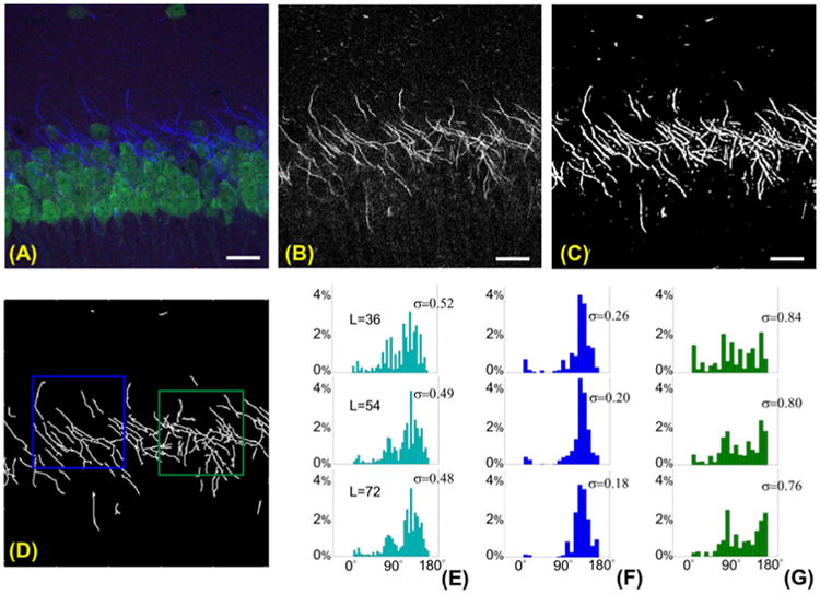
Multiscale estimation of orientation of axons of CA1 neurons. (A): Multichannel confocal image of CA1 hippocampal region in Maximum Projection view. Image size: 512 × 512. (B): Blue channel from panel (A) showing the axons, (C) corresponding segmented image and (D) centerline traces. Two ROIs are manually selected in panel (D) to process directional information. (E) Histograms of the orientations of the segmented axons in panel (C) for orientation angles between 0° and 180° at multiple scales, where L denotes the length of the filter in pixels. The vertical axis indicates the percentage of measures counted in each bin. Panels (F) and (G) show the histograms of orientations, at multiple scales, for the for the ROIs selected in panel (D), with matching blue and green colors. The value of σ reported next to each histogram is the circular variance for the measured angles. Angles are pooled into 5° bins from 0° to 180° in (E); angles are pooled into 10° bins from 0° to 180° in (F-G). In (A-C), scale bar: 20 μm.

Additional data we considered include immunofluorescent images of spinal cord tissue where axons were labeled with βIII-tubulin. This set of data was kindly provided by the lab of Dr. Blesch from the Spinal Cord Injury Center at the Heidelberg University and are part of the images analyzed in the AngleJ paper (Günther et al, 2015). A representative example is shown in Fig. 6 where an image containing βIII-tubulin labeled neurites is segmented (panel (B)) and traced to generate the histograms of orientations at multiple scales (panel (C)). For comparison, we also include the histograms of orientations computed using the AngleJ algorithm for different values of the smoothing parameter s (panel (D)). Even though AngleJ does not provide a proper multiscale framework, by changing the parameter s one can essentially change the ‘scale’ of the filtering process multi-scale (larger s corresponds to more blurring). The computation of the EMD-alignment score for the image using filters of length L = 36, 54, 72 yields ν^(EMD) = 0.174, 0.142, 0.140, respectively.

Fig. 6. Orientation estimation: our approach vs. AngleJ.

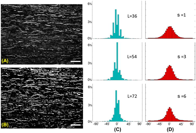
(A) Image of βIII-tubulin labeled neurites (image size is 1028 × 760 pixels) and (B) its segmented binary image. (C) Corresponding histograms of orientations, for orientation angles between −90° and 90°, computed using our algorithm at different scales; here L denotes the length of the filter in pixels. (D) Histograms of orientations computed using the AngleJ algorithm using different parameters s for the Gaussian blurring preprocessing filter. In (C-D) angles are pooled into 5° bins from −90° to 90°. The vertical axis indicates the percentage of measures counted in each bin. In (A-B), scale bar: 50 μm.

To illustrate the ability of the alignment score to discriminate images of vessel-like structures based on their orientation pattern, we run our algorithm for the extraction of neurite orientation on fluorescence images coming from multiple experiments and computed their EMD-alignment score. Results are shown in Fig. 7. That second through fifth images in Fig. 7 show βIII-tubulin labeled axons from the AngleJ paper (Günther et al, 2015), as in Fig. 6, and exhibit comparable values of EMD-alignment score. Similarly the sixth through eight images show axons of CA1 neurons as in Fig. 5 and also exhibit comparable values of EMD-alignment score. The same observation holds for the first three images in the second row Fig. 7, which show axons from the dentate gyrus. To generate all these results we used filter length L = 54.

Fig. 7. Alignment score.

The figure shows 16 images, both synthetic and experimental ones, ordered according to their computed EMD-based alignment score which is reported below the corresponding image.

3.3 Computational cost, hardware and software

We implemented the numerical codes for the algorithms presented above using Python. The numerical tests were performed using a LENOVO ThinkPad X220 Tablet, with OS Ubuntu 14.04 TLS, 64 bit CPU, Intel(R) Core(TM) i5-2520M CPU at 2.50GHz and 4 GB RAM. Since the algorithms are highly parallelizable, the code would run significantly faster using multi-CPU architecture. However, even with our single-CPU system, computation times were very reasonable.

As mentioned above, our segmentation routine is based on an SVM approach which requires a training stage to compute a classifier model. This stage needs to be run only once for a given type of data (same cell type and microscopy setting). Its computation is automated and takes about 8 hours on our system. After this stage, the segmentation of a 512 × 512 image takes about 2 sec.

On the synthetic images from Fig. 3, where each image has size 512 × 512 pixels, the extraction of centerline curves takes between 0.09116 and 2.1081 sec; the computation of local orientation angles (using 16 directional bands) takes between 0.4103 and 6.5219 sec; the computation of the ℓ²-based alignment score takes between 0.0005 and 0.0011 sec; the computation of the EMD-based alignment score takes between 0.0029 and 0.0057 sec. The difference in computation time depends on the complexity of the image. In fact, as noted above, each disconnected component of the segmented is processed separately.

On the experimental image in Fig. 5, of size 512 × 512 pixels, the extraction of centerline curves takes 1.0006 sec; the computation of local orientation angles (using 16 directional bands) takes 5.8714 sec; the computation of the ℓ²-based alignment score takes 1.5944 sec; the computation of the EMD-based alignment score takes 0.0065 sec.

The Python code used to generate our results, as well as our data, are publicly available at https://github.com/psnegi/NeuriteOrientation.

Our implementation of the EMD distance follows the algorithm by Pele and Werman (Pele and Werman, 2009).

4 Discussion and conclusion

We have introduced an algorithm for the automated computation of the orientation of neurites in images of neurons in culture and tissue, and successfully validated its performance on both synthetic and experimental data.

Similar to other image analysis algorithms for neuronal data, our method relies on a segmentation routine to extract neurons from background. The overall performance of our orientation estimation algorithm depends on the performance of the segmentation routine since orientation estimation is only applied to segmented structures. Even though, as discussed above, our segmentation routine is very reliable, it is still possible that, due to nonuniformities of the fluorescent signal intensity, some neurite sections are lost with the result that corresponding neurites appear broken. Fortunately, this is not a significant problem for our algorithm, as it is designed to compute local orientation for all segmented vessel-like structures even if limited to sections of neurites. We recall that our directional filters are centered along the coordinates of the centerline of segmented neurites. Possible errors in the location of the centerline, e.g., a shift by one or two pixels, have very low impact on the estimation of local orientation, since directional filters remain sensitive to the geometry of a vessel-like structure even if they are not located exactly on the centerline. In practice, errors in the extraction of the centerline only occur in the presence of crossing neurites or branching points. Those points are rare in our data.

With respect to existing algorithms targeted to the analysis of neurite orientation (e.g., AngleJ and Neurient), one major novelty of our approach is the application of a set of multiscale directional filters designed to assess the physical orientation of neurites and distinguish this property from small scale oscillations due to noise and irregularities in the image, e.g., non-uniformity in the fluorescent signal. Our method automatically selects the range of scales of interest based on geometric parameters computed from the images. In addition, the algorithm is designed to processes one neurite at a time so that directional filtering is not affected by the presence of neighbouring neurites.

Even though existing algorithms for the automated computation of neurites orientation do not explicitly carry over a multiscale estimation, they often apply a smoothing operator to images producing an effect similar to dilation. For instance, the AngleJ algorithm (Günther et al, 2015) applies Gaussian blurring, dependent on a blurring parameter s > 0, before the actual estimation of neurite orientation, acting essentially as isotropic dilation. When combined with directional estimation, by varying the s parameter one obtains results comparable to a multiscale directional filtering. This effect is shown in Figure 8 illustrating the application of the AngleJ algorithm to the same set of synthetic images considered in Figure 1 for several values of the blurring parameter s. Similar to our multiscale approach (in Figure 1), results in Figure 8 show that the algorithm becomes less sensitive to local oscillations of the synthetic neurite when s increases. However, the estimate of orientation is not very accurate as multiple peaks appear around the angle θ = 0. For example, in panel C, as the parameter s increases, multiple significant directional components appear in the histogram unlike our result in Figure 1 where our method provides accurate angle estimation selectivity even at coarser scales. The superior performance of our approach is due to the properties of our directional filters, which are associated with anisotropic (rather than isotropic) dilations to ensure high directional selectivity at all scales.

Fig. 8. Multiscale analysis of orientation.

The figure illustrates the histograms of the orientations of synthetic models of neurites (panels A-C), for orientation angles between −90° and 90° using Gaussian smoothing filters (from AngleJ) with different smoothing parameter s. Angles are pooled into 10° bins and the vertical axis of the histogram indicates the percentage of orientation angles counted in each bin. At the finest scale (s = 1), the histograms of orientation are similar and show two dominant orientations for all images. At coarser scales (s = 3, 6), the histograms show a different behavior for each image.

Another major novel contribution of this paper is the notion of alignment score, proposed as a practical measure of the degree of co-alignment and spatial organization of neurites. This concept is quite novel and conceptually different from other geometric descriptors proposed in the literature for the analysis of vessel-like structures, such as the Sholl (Langhammer et al, 2010; Sholl, 1953) and fractal analysis (Milošević et al, 2005), which were designed to measure the branching density and ramification richness of neurons rather than their alignment properties.

Even though we illustrated the application of our algorithm on standard 2D images, the method we presented extends naturally to the 3D setting. In fact, the segmentation and centerline tracing steps of the algorithm, which are adapted from our previous work in Jimenez et al (2013, 2015a) and Ozcan et al (2015), is already available both in the 2D and 3D settings. The extension of directional filtering to 3D is conceptually straightforward. In fact, rectangular steerable filters can be defined in 3D similar to the construction above. The main difference is that 3D rotations will be controlled by two angles, the polar angle φ and the azimuthal angle θ, so that the new directional response H f (j, θ_m, ϕ_n, k), defined as in equation (1), will depend on two angular parameters rather than a single one. An example of application of our method to compute a histogram of orientations in the 3D setting using a simple synthetic image is shown in Figure 9.

Fig. 9. Orientation estimation in 3D.

The figure illustrates a synthetic model of a neurite in the 3D setting (left panel) and the corresponding histogram of the orientations (on the left), for orientation angles ranging from 0° to 90° for the polar angle φ and 0° to 180° for the azimuthal angle θ. Angles are pooled into 9° bins for φ, into 18° bins for θ. Histogram indicates the number of orientation angles counted in each bin.

The computational cost of directional filtering, which is not a concern in 2D, requires much more care in the 3D setting. In fact, even when selecting only 10 samples per angular direction as in the simple example in Figure 9, this choice already produces 100 discretized directions. Hence, for each voxel located on the centerline of the neurite, we need to compute 100 3D convolutions.

Recall that, in 2D, directional filtering for an image of size N × N requires (using FFT to implement convolution) about N² logN operations. Using M directions, this brings the total of operation to MN² logN. Using the same approach in 3D, with the same density of directions, the computational cost would be M²N³ logN operations, which would make data processing very time-consuming. To reduce computational cost, it is possible to produce directional filtering based on anisotropic Gaussian filters rather than rectangular ones. A number of papers have shown that it is possible to derive separable implementations of such filters bringing down the computational cost to about 2MN logN operations in the 2D case and about 3M²N logN operations in the 3D case (Geusebroek et al, 2003; Lampert and Wirjadi, 2006; Yiu Man Lam and Shi, 2007).

The algorithms presented in this paper apply to a wide range of images containing vessel-like structures going beyond the types of data considered in this paper. In case images contain additional structures such as somas or other blob-like objects, our algorithms can be applied after first removing such blob-like structures from the segmented images. This task can be addressed, for instance, by using a method for automated soma detection and segmentation recently developed by some of the authors (Ozcan et al, 2015). This method uses a geometric descriptor called ‘directionality ratio’ to automatically separate vessel-like structure from more isotropic ones and was successfully applied to automatically separate somas from neurites in confocal images of neuronal cultures and brain tissue.

In conclusion, the method and ideas presented in this paper offer an innovative automated tool for image analysis applicable to a wide range of problems where it is important to extract directionality and quantify spatial distribution of vessel-like structures. We expect that this method will provide a very valuable tool for the analysis of large-scale data sets from problems in neuroregeneration, the study of the connectome and other neuroscience research projects. The application of the quantitative methods presented for the analysis of long-range neurite growth and the study of vessel-like structures in healthy and diseased conditions will be pursued in future studies.

References

- 3D-Slicer. 2008 Http://www.slicer.org/
- Al-Kofahi KA, Lasek S, Szarowski DH, Pace CJ, Nagy G, Turner JN, Roysam B. Rapid automated three-dimensional tracing of neurons from confocal image stacks. Trans Info Tech Biomed. 2002;6(2):171–187. doi: 10.1109/titb.2002.1006304. [DOI] [PubMed] [Google Scholar]
- Chothani P, Mehta V, Stepanyants A. Automated tracing of neurites from light microscopy stacks of images. Neuroinformatics. 2011;9(2-3):263–278. doi: 10.1007/s12021-011-9121-2. [DOI] [PMC free article] [PubMed] [Google Scholar]
- Debanne D, Campanac E, Bialowas A, Carlier E, Alcaraz G. Axon physiology. Physiological reviews. 2011;91(2):555–602. doi: 10.1152/physrev.00048.2009. [DOI] [PubMed] [Google Scholar]
- Easley GR, Labate D, Lim W. Sparse directional image representations using the discrete shearlet transform. Appl Numer Harmon Anal. 2008;25:25–46. [Google Scholar]
- Geusebroek JM, Smeulders A, van de Weijer J. Fast anisotropic gauss filtering. Image Processing, IEEE Transactions on. 2003;12(8):938–943. doi: 10.1109/TIP.2003.812429. [DOI] [PubMed] [Google Scholar]
- Günther MI, Günther M, Schneiders M, Rupp R, Blesch A. AngleJ: A new tool for the automated measurement of neurite growth orientation in tissue sections. Journal of Neuroscience Methods. 2015;251:143–150. doi: 10.1016/j.jneumeth.2015.05.021. [DOI] [PubMed] [Google Scholar]
- Hines M, Carnevale N. NEURON: a tool for neuroscientists. The Neuroscientist. 2001;7:123–135. doi: 10.1177/107385840100700207. [DOI] [PubMed] [Google Scholar]
- Jimenez D, Papadakis M, Labate D, Kakadiaris I. Improved automatic centerline tracing for dendritic structures. Biomedical Imaging (ISBI), 2013 IEEE 10th International Symposium on. 2013:1050–1053. [Google Scholar]
- Jimenez D, Labate D, Kakadiaris IA, Papadakis M. Improved automatic centerline tracing for dendritic and axonal structures. Neuroinformatics. 2015a;13(2):227–244. doi: 10.1007/s12021-014-9256-z. [DOI] [PubMed] [Google Scholar]
- Jimenez D, Labate D, Papadakis M. Directional analysis of 3D tubular structures via isotropic well-localized atoms. Appl Comput Harmon Anal. 2015b in press. [Google Scholar]
- Kullback S. Information Theory and Statistics. Dover Publications; 1997. [Google Scholar]
- Lampert CH, Wirjadi O. An optimal nonorthogonal separation of the anisotropic gaussian convolution filter. Image Processing, IEEE Transactions on. 2006;15(11):3501–3513. doi: 10.1109/tip.2006.877501. [DOI] [PubMed] [Google Scholar]
- Langhammer CG, Previtera ML, Sweet ES, Sran SS, Chen M, Firestein BL. Automated sholl analysis of digitized neuronal morphology at multiple scales: whole cell sholl analysis versus sholl analysis of arbor subregions. Cytometry Part A. 2010;77(12):1160–1168. doi: 10.1002/cyto.a.20954. [DOI] [PMC free article] [PubMed] [Google Scholar]
- Ling H, Okada K. An efficient earth mover's distance algorithm for robust histogram comparison. Pattern Analysis and Machine Intelligence, IEEE Transactions on. 2007;29(5):840–853. doi: 10.1109/TPAMI.2007.1058. [DOI] [PubMed] [Google Scholar]
- Lledo PM, Alonso M, Grubb MS. Adult neurogenesis and functional plasticity in neuronal circuits. Nature Reviews Neuroscience. 2006;7(3):179–193. doi: 10.1038/nrn1867. [DOI] [PubMed] [Google Scholar]
- Luisi J, Narayanaswamy A, Galbreath Z, Roysam B. The FARSIGHT trace editor: an open source tool for 3-D inspection and efficient pattern analysis aided editing of automated neuronal reconstructions. Neuroinformatics. 2011;9(2-3):305–315. doi: 10.1007/s12021-011-9115-0. [DOI] [PubMed] [Google Scholar]
- Mahoney MJ, Chen RR, Tan J, Saltzman WM. The influence of microchannels on neurite growth and architecture. Biomaterials. 2005;26(7):771–778. doi: 10.1016/j.biomaterials.2004.03.015. [DOI] [PubMed] [Google Scholar]
- Milošević NT, Ristanović D, Stanković J. Fractal analysis of the laminar organization of spinal cord neurons. Journal of neuroscience methods. 2005;146(2):198–204. doi: 10.1016/j.jneumeth.2005.02.009. [DOI] [PubMed] [Google Scholar]
- Mitchel JA, Martin IS, Hoffman-Kim D. Neurient: An algorithm for automatic tracing of confluent neuronal images to determine alignment. Journal of Neuroscience Methods. 2013;214(2):210–222. doi: 10.1016/j.jneumeth.2013.01.023. [DOI] [PMC free article] [PubMed] [Google Scholar]
- Ozcan B, Negi P, Laezza F, Papadakis M, Labate D. Automated detection of soma location and morphology in neuronal network cultures. PloS One. 2015;10(4) doi: 10.1371/journal.pone.0121886. [DOI] [PMC free article] [PubMed] [Google Scholar]
- Pele O, Werman M. 2009 IEEE 12th International Conference on Computer Vision. IEEE; 2009. Fast and robust earth mover's distances; pp. 460–467. [Google Scholar]
- Peng H, Long F, Myers G. Automatic 3D neuron tracing using all-path pruning. Bioinformatics. 2011;27(13):i239. doi: 10.1093/bioinformatics/btr237. [DOI] [PMC free article] [PubMed] [Google Scholar]
- Portera-Cailliau C, Weimer RM, De Paola V, Caroni P, Svoboda K. Diverse modes of axon elaboration in the developing neocortex. PLoS biology. 2005;3(8):1473. doi: 10.1371/journal.pbio.0030272. [DOI] [PMC free article] [PubMed] [Google Scholar]
- Rossi F, Gianola S, Corvetti L. Regulation of intrinsic neuronal properties for axon growth and regeneration. Prog Neurobiol. 2007;81(1):1–28. doi: 10.1016/j.pneurobio.2006.12.001. [DOI] [PubMed] [Google Scholar]
- Rubner Y, Tomasi C, Guibas LJ. A metric for distributions with applications to image databases. ICCV. 1998:59–66. [Google Scholar]
- Rubner Y, Tomasi C, Guibas LJ. The earth mover's distance as a metric for image retrieval. Int J Comput Vision. 2000;40(2):99–121. [Google Scholar]
- Santamaria A, Colbert C, Losavio B, Saggau P, Kakadiaris I. Proc International Workshop in Microscopic Image Analysis and Applications in Biology. Piscataway, NJ: 2007. Automatic morphological reconstruction of neurons from optical images. [Google Scholar]
- Saxena S, Caroni P. Mechanisms of axon degeneration: From development to disease. Progress in Neurobiology. 2007;83(3):174–191. doi: 10.1016/j.pneurobio.2007.07.007. [DOI] [PubMed] [Google Scholar]
- Scorcioni R, Polavaram S, Ascoli G. L-measure: a web-accessible tool for the analysis, comparison and search of digital reconstructions of neuronal morphologies. Nature Protocols. 2008;3(5):866–876. doi: 10.1038/nprot.2008.51. [DOI] [PMC free article] [PubMed] [Google Scholar]
- Shavkunov AS, Wildburger NC, Nenov MN, James TF, Buzhdygan TP, Panova-Elektronova NI, Green TA, Veselenak RL, Bourne N, Laezza F. The fibroblast growth factor 14voltage-gated sodium channel complex is a new target of glycogen synthase kinase 3 (GSK3) J Biol Chem. 2013;288(27):19,370–85. doi: 10.1074/jbc.M112.445924. [DOI] [PMC free article] [PubMed] [Google Scholar]
- Sholl D. Dendritic organization in the neurons of the visual and motor cortices of the cat. Journal of anatomy. 1953;87(Pt 4):387. [PMC free article] [PubMed] [Google Scholar]
- Walsh JF, Manwaring ME, Tresco PA. Directional neurite outgrowth is enhanced by engineered meningeal cell-coated substrates. Tissue engineering. 2005;11(7-8):1085–1094. doi: 10.1089/ten.2005.11.1085. [DOI] [PubMed] [Google Scholar]
- Yiu Man Lam S, Shi B. Recursive anisotropic 2-d gaussian filtering based on a triple-axis decomposition. Image Processing, IEEE Transactions on. 2007;16(7):1925–1930. doi: 10.1109/tip.2007.896673. [DOI] [PubMed] [Google Scholar]