Optimum Diffraction-Corrected Frequency-Shift Estimator of the Ultrasonic Attenuation Coefficient

Abstract

The ultrasonic attenuation coefficient is an important parameter that has been studied extensively in Quantitative Ultrasound and Tissue Characterization. There are various methods described in the literature that estimate this parameter by measuring either spectral difference (i.e., decay) or spectral shift of the backscattered echo signal. Under ideal conditions, i.e., in the absence of abrupt changes in tissue backscattering, Spectral Difference methods can produce estimates with high accuracy and precision. On the other hand, diffraction-corrected Spectral Shift methods (e.g., the Hybrid method) are better suited for application in practical settings using clinical ultrasound scanners. However, current Spectral Shift methods use inefficient frequency shift estimators that ultimately degrade the quality of attenuation coefficient estimates. In this paper, a probabilistic model of the backscattered radiofrequency (RF) echo is used to derive the Cramér-Rao lower bound (CRLB) on estimation variance of the spectral centroid. Next, an efficient correlation-based shift estimator is presented that achieves the CRLB. Used in conjunction with a well-characterized reference phantom to correct for diffraction and other system-related effects, this estimator greatly improves the accuracy and precision of Spectral-Shift attenuation estimation. A theoretical analysis of this method is provided, and its performance is quantitatively compared with that of the Hybrid method using simulated and experimental phantom studies. A minimum of 3-fold reduction in the standard deviation of attenuation coefficient estimates is observed using the new method.

I. Introduction

Accurate estimation of the ultrasonic attenuation coefficient has numerous clinical and non-clinical benefits. In addition to providing potentially valuable diagnostic information, localized estimation of the attenuation coefficient and compensation for it can significantly improve the quality of estimation for other acoustic parameters of interest in Quantitative Ultrasound (QUS) and Tissue Characterization [1], [2]. The attenuation coefficient has been studied as a classifier of normal and pathological conditions in fatty liver [3]–[7], breast tissue [8], [9], myocardial tissue [10]–[12], carotid artery plaques [13]–[15], osteoporosis [16], [17], and deep vein thrombosis [18], [19].

Spectral methods of attenuation estimation are favored over time-domain methods because they allow for easier correction for equipment-related diffraction effects and frequency-specific estimation. These methods estimate the change of spectral content with depth. Spectral Difference methods measure the log-intensity decay at each frequency point [20], [21], and Spectral Shift methods measure the frequency downshift of the spectral centroid [22], [23].

The challenge with estimating the attenuation coefficient is that attenuation is not the only mechanism by which the spectral content evolves with depth. Diffraction effects due to ultrasound field inhomogeneity and scattering effects due to propagation medium inhomogeneity also alter the echo signal spectrum. These effects may be both frequency- and depth-dependent. In order to improve the quality of attenuation estimation, many investigators have introduced methods that attempt to account for or eliminate these spectral effects [24], [25]. The Reference Phantom Method (RPM) is a widely used approach to eliminating system-related diffraction effects [26]. However, it does not account for the scattering effects associated with sample medium inhomogeneity, and this limits the applicability of Spectral Difference methods in clinical settings. Spectral Shift methods are also affected by scattering variations in the medium, but only if these variations change the frequency dependence of the spectral profile. In other words, unlike the Spectral Difference category, a simple frequency-independent amplitude gain or loss is not enough to introduce bias to estimations of the Spectral Shift category. Kim, et al. [27] combined the use of a reference phantom with spectral shift estimation in their Hybrid method and reported improvements on attenuation estimation in inhomogeneous sample media compared to either Spectral Difference or conventional Spectral Shift methods.

Despite these improvements, the estimation variance is still too high to provide reliable attenuation coefficient maps with acceptable spatial resolution that could be implemented on clinical scanners. Some authors have focused on optimizing the periodogram-based estimation of the echo signal power spectrum by investigating various gating window functions [28], thus improving subsequent QUS parameter estimations. However, it can be argued that the most critical step for attenuation estimation using Spectral Shift methods is to accurately determine the spectral centroid and its shift. Different approaches to finding the center frequency are described in ultrasound and Doppler radar literature [29], [30]. These range from the simple zero-crossing technique to energy balancing [30], centroid detection using the method of moments [22], and correlation-based techniques [29], [30], [25]. Many researchers in the field of ultrasound have used the method of moments for centroid detection. While this method is computationally inexpensive, it is not an efficient estimator of the spectral shifts. Kim et al. [25], [27] used a correlation-based shift estimator for their Hybrid method, claiming that it provides more accurate and robust estimations than the method of moments. Other authors have implemented the Hybrid method with minor adjustments [31] or by replacing the cross-correlation step with the method of moments [32] and reported improvements.

In this paper, we present an optimum frequency shift estimator that significantly improves the stability of the Hybrid method for attenuation estimation using clinical scanners. The following background section presents fundamental information on efficient centroid detection using a correlation-based estimator from the literature [30]. The materials and methods section applies these ideas in the context of ultrasonic attenuation coefficient estimation using a reference phantom. The result is a maximum-likelihood (ML) attenuation estimation method that combines the benefits of spectral normalization using a reference phantom with the robustness of Spectral Shift estimators of the attenuation coefficient. Finally, we quantitatively compare the performance of our method with the Hybrid method as well as with an improved implementation of the Hybrid method. The comparisons use simulated and experimental Radio Frequency (RF) data.

II. Background

A. Spectral Centroid Estimation Preliminaries

Consider the ultrasonic echo signal received by the transducer and sampled at a period of T_s to form the complex vector:

$$x=\left(x\right[0],x[1],\dots ,x[M-1\left]\right),$$ (1)

where x is an M-point segment of an RF A-line and is assumed to constitute a complex, Gaussian, zero-mean, and stationary process. The discrete Fourier transform (DFT) of x, therefore, constitutes a complex, Gaussian, zero-mean process, X. Due to stationarity of x, the spectral samples X[i] are mutually uncorrelated.

$$X=\left(X\right[0],X[1],\dots ,X[M-1\left]\right).$$ (2)

Since the phase of X contains no information about the center frequency, it is sufficient to consider the power spectrum, S, in order to estimate the spectral centroid.

$$\begin{array}{cc}\hfill S& =\left(S\right[0],S[1],\dots ,S[M-1\left]\right)\hfill \\ \hfill & =\left({\mid X\left[0\right]\mid }^2,{\mid X\left[1\right]\mid }^2,\dots ,{\mid X[M-1]\mid }^2\right).\hfill \end{array}$$ (3)

The expected value of the power spectral sample S[i] is given by (4).

$$\mathrm{E}\left[S\right[i\left]\right]=A(i\cdot \Delta f-f_c),$$ (4)

where A(f) is the nominal power spectrum and is periodic with frequency F_s = 1/T_s. Under diffuse scattering conditions, X is a complex Gaussian process. Therefore, each sample of the power spectral density, S[i], will have an exponential (chi-squared with two degrees of freedom) probability density function (pdf) given by (5) which results in typical speckle statistics [33]. The variance of S[i] is thus written as (6).

$$p(S[i];f_c)=\frac{1}{A(i\cdot \Delta f-f_c)}\cdot \exp \left(-\frac{S\left[i\right]}{A(i\cdot \Delta f-f_c)}\right),$$ (5)

$$\mathrm{Var}\left(S\right[i\left]\right)=A^2(i\cdot \Delta f-f_c).$$ (6)

B. The Cramér-Rao Lower Bound for Centroid Estimation

It is known from estimation theory [34] that the variance of any unbiased estimator of the centroid frequency has a lower bound given by the Cramér-Rao inequality:

$$\mathrm{Var}\left(\widehat{f_c}\right)\ge \frac{1}{\mathrm{E}\left[{\left(\frac{\partial \ln p(S;f_c)}{\partial f_c}\right)}^2\right]},$$ (7)

where p(S; f_c) is the joint pdf for all S[i] with parameter f_c. This lower bound can easily be evaluated for the centroid estimation problem defined above. The resulting CRLB is given by (8) in terms of the nominal power spectrum, A. Integration is performed over one spectral period, F_s.

$$\mathrm{Var}\left(\widehat{f_c}\right)\ge \frac{\Delta f}{\int {\left[\frac{A^{\prime }\left(f\right)}{A\left(f\right)}\right]}^{2}df}.$$ (8)

C. Correlation-Based Centroid Estimators

This category of centroid estimators relies on correlating the power spectrum, S, with some weighting function, B, centered at a trial centroid, $\widehat{f_c}$, and looking for a zero.

$$C\left(\widehat{f_c}\right)=\sum _{i=0}^{M-1}S[i]\cdot B\left(i\cdot \Delta f-\widehat{f_c}\right).$$ (9)

The value of $\widehat{f_c}$ with $C\left(\widehat{f_c}\right)=0$ is taken as the centroid estimate. It is clear that the performance of such an estimator is dependent on the choice of weighting function B.

In order to derive the variance of the centroid estimate $\widehat{f_c}$, we study the statistics of the correlation function of (9). $C\left(\widehat{f_c}\right)$ is a weighted sum of uncorrelated power spectral samples S[i]. Therefore, $C\left(\widehat{f_c}\right)$ is a random process with a distribution that approaches a Gaussian distribution, due to the Central Limit Theorem, as M increases. Its expected value can be written as (10).

$$\begin{array}{cc}\hfill \mathrm{E}\left[C\left(\widehat{f_c}\right)\right]& =\sum _{i=0}^{M-1}A(i\cdot \Delta f-f_c)\cdot B\left(i\cdot \Delta f-\widehat{f_c}\right)\hfill \\ \hfill & \simeq \frac{1}{\Delta f}\cdot \int A(f-f_c)\cdot B\left(f-\widehat{f_c}\right)df,\hfill \end{array}$$ (10)

Using (6), the variance is given by (11).

$$\begin{array}{cc}\hfill \mathrm{Var}\left(C\left(\widehat{f_c}\right)\right)& =\sum _{i=0}^{M-1}{A}^2(i\cdot \Delta f-f_c)\cdot B^2\left(i\cdot \Delta f-\widehat{f_c}\right)\hfill \\ \hfill & \simeq \frac{1}{\Delta f}\cdot \int {\left[A(f-f_c)\cdot B\left(f-\widehat{f_c}\right)\right]}^{2}df.\hfill \end{array}$$ (11)

In the vicinity of $\widehat{f_c}=f_c$, a first-order Taylor series expansion can be written for $\mathrm{E}\left[C\right(\widehat{f_c}\left)\right]$ as seen in (12).

$$\mathrm{E}\left[C\left(\widehat{f_c}\right)\right]=k\cdot \left(\widehat{f_c}-f_c\right)+\cdots$$ (12)

with

$$\begin{array}{cc}\hfill k={\phantom{\mid }\frac{d\mathrm{E}\left[C\left(\widehat{f_c}\right)\right]}{d\widehat{f_c}}\mid }_{\widehat{f_c}=f_c}& \simeq \frac{-1}{\Delta f}\cdot \int A\left(f\right)\cdot B^{\prime }\left(f\right)df\hfill \\ \hfill & =\frac{1}{\Delta f}\cdot \int A^{\prime }\left(f\right)\cdot B\left(f\right)df.\hfill \end{array}$$ (13)

The last equation in (13) holds due to periodicity of A and B with period F_s which is also the integration interval. Therefore, the variance of the centroid estimate is given by (14). The centroid estimate, $\widehat{f_c}$, is also Gaussian distributed if the number of data points, M, is sufficiently large.

$$\begin{array}{cc}\hfill \mathrm{Var}\left(\widehat{f_c}\right)& \simeq \frac{\mathrm{Var}\left(C\right(f_c\left)\right)}{k^2}\hfill \\ \hfill & =\Delta f\cdot \frac{\int {\left[A\right(f)\cdot B(f\left)\right]}^{2}df}{{\left[\int A\left(f\right)\cdot B^{\prime }\left(f\right)df\right]}^2}\hfill \\ \hfill & =\Delta f\cdot \frac{\int {\left[A\right(f)\cdot B(f\left)\right]}^{2}df}{{\left[\int A^{\prime }\left(f\right)\cdot B\left(f\right)df\right]}^2}.\hfill \end{array}$$ (14)

D. The Optimum Centroid Estimator

It has been shown in the literature [30] that the maximum-likelihood estimator of the centroid that achieves the Cramér-Rao bound is a correlation-based estimator as defined in (9) that uses the following weighting function:

$$B(f)=-\frac{d}{df}\left(\frac{1}{A\left(f\right)}\right)=\frac{A^{\prime }\left(f\right)}{A^2\left(f\right)}.$$ (15)

Note that inserting the weighting function from (15) into (14) results in an estimation variance equal to the CRLB from (8).

The maximum-likelihood estimator looks for the zero of the correlation between the measured power spectrum and the derivative of 1/ A(f). This is equivalent to minimization of the correlation between the measured spectrum and the reciprocal of the nominal power spectrum. Intuitively interpreted, this means that areas of the power spectrum with high energy, and therefore with high speckle noise, get a smaller weight in the correlation step than low-energy areas of the power spectrum with low speckle noise. This concept explains the superior performance of this estimator for signals, such as ultrasound echo, that experience multiplicative noise.

III. Materials and Methods

A. Statistical Analysis of the Normalized Power Spectrum

In order to estimate ultrasonic attenuation with use of a reference phantom, frames of RF data are acquired using the exact same scan settings (i.e., depth, focus, gain, transmit power, etc.) from both the sample and a well-characterized reference phantom. The RF data frames are partitioned into blocks consisting of data from several adjacent echo lines that have been windowed at each depth point using a time-gating window function of appropriate length. These windowed data segments are then Fourier transformed, squared, and averaged to obtain estimates of the signal power spectrum from each block. The power spectrum corresponding to a block at depth z of a homogenous sample is modeled as (16).

$$S_S(f,z)=S_t\left(f\right)D(f,z){\mathit{BSC}}_S(f,z)e^{-4{\alpha }_S\left(f\right)z}.$$ (16)

In this equation, S_t(f) represents the transmit pulse and transfer functions associated with the boundary between the transducer and sample. D(f, z) denotes the diffraction effects that are linked with transducer geometry and beam-forming. BSC_S(f, z) is the backscatter coefficient spectral profile of random scatterers in the sample medium. e^−4α_S(f)z is the cumulative attenuation at frequency f and depth z. Similarly, the power spectrum from a block at depth z of the reference phantom is modeled as (17).

$$S_R(f,z)=S_t\left(f\right)D(f,z){\mathit{BSC}}_R(f,z)e^{-4{\alpha }_R\left(f\right)z}.$$ (17)

Since system settings for both data acquisitions are identical, transmit and diffraction terms are the same in (16) and (17). Therefore, normalizing the sample power spectrum by the reference power spectrum cancels these terms out. The ratio of power spectra is given in (18).

$$\mathit{RS}(f,z)=\frac{S_S(f,z)}{S_R(f,z)}=\frac{{\mathit{BSC}}_S(f,z)e^{-4{\alpha }_S\left(f\right)z}}{{\mathit{BSC}}_R(f,z)e^{-4{\alpha }_R\left(f\right)z}}.$$ (18)

We will assume a linearly frequency-dependent attenuation profile, α(f)=β·f, for both sample and reference materials.

The backscatter spectral term is modeled as a Chi-square distributed random process [35]–[37] with a pdf given by (19).

$$p\left(\mathit{BSC}\right(f,z\left)\right)=\frac{1}{{\sigma }^2}\exp \left(-\frac{\mathit{BSC}(f,z)}{{\sigma }^2}\right),\mathit{BSC}(f,z)\ge 0.$$ (19)

Therefore, it will have mean E[BSC(f, z)] = σ² and variance Var(BSC(f, z)) = σ⁴. If the spectra from multiple (N) adjacent A-lines are averaged prior to normalization, the averaged backscatter term will be Gamma distributed, as shown in (20).

$$\overline{\mathit{BSC}}(f,z)=\frac{1}{N}\sum _{i=1}^N{\mathit{BSC}}^{\left(i\right)}(f,z)\sim \Gamma \left(\frac{N}{2},\frac{2{\sigma }^2}{N}\right).$$ (20)

For a sufficiently large N, this Gamma distribution can be approximated by a Normal distribution. Therefore, the averaged backscatter terms for sample and reference spectra are modeled as (21). This approximation can also be directly made according to the Central Limit Theorem.

$$\begin{array}{cc}\hfill & \overline{{\mathit{BSC}}_S}(f,z)\sim \mathcal{N}\left({{\sigma }_S}^2,\frac{2{{\sigma }_S}^4}{N_S}\right),\hfill \\ \hfill & \overline{{\mathit{BSC}}_R}(f,z)\sim \mathcal{N}\left({{\sigma }_R}^2,\frac{2{{\sigma }_R}^4}{N_R}\right).\hfill \end{array}$$ (21)

The ratio of the uncorrelated non-zero mean Gaussian random variables from (21) has a complicated distribution and pdf. Therefore, going forward, we make the assumption that this “ratio random variable”, RB(f, z), is normally distributed about its mean value. The validity of this approximation can be verified by comparing it to the ratio of two Gamma-distributed random variables of the form given in (20) as N grows. The verification has been performed but is not presented, as it is beyond the scope of this paper. We approximate the mean value and the variance using first or second order Taylor expansions of the ratio function. Using a first-order Taylor expansion of the ratio function, the mean value is given by (22).

$${\mu }_{\mathit{RB}}=\mathrm{E}\left[\mathit{RB}(f,z)\right]\approx \frac{\mathrm{E}\left[\overline{{\mathit{BSC}}_S}(f,z)\right]}{\mathrm{E}\left[\overline{{\mathit{BSC}}_R}(f,z)\right]}=\frac{{{\sigma }_S}^2}{{{\sigma }_R}^2}.$$ (22)

Using a second-order Taylor expansion of the ratio function, the mean value is given by (23).

$$\begin{array}{cc}\hfill {\mu }_{\mathit{RB}}& =\mathrm{E}\left[\mathit{RB}(f,z)\right]\hfill \\ \hfill & \approx \frac{\mathrm{E}\left[\overline{{\mathit{BSC}}_S}\right]}{\mathrm{E}\left[\overline{{\mathit{BSC}}_R}\right]}-\frac{\mathrm{Cov}\left(\overline{{\mathit{BSC}}_S},\overline{{\mathit{BSC}}_R}\right)}{{\mathrm{E}}^2\left[\overline{{\mathit{BSC}}_R}\right]}+\frac{\mathrm{Var}\left(\overline{{\mathit{BSC}}_R}\right)\mathrm{E}\left[\overline{{\mathit{BSC}}_S}\right]}{{\mathrm{E}}^3\left[\overline{{\mathit{BSC}}_R}\right]}\hfill \\ \hfill & =\frac{{{\sigma }_S}^2}{{{\sigma }_R}^2}-0+\frac{2{{\sigma }_R}^4{{\sigma }_S}^2}{N_R{{\sigma }_R}^6}=\frac{{{\sigma }_S}^2}{{{\sigma }_R}^2}\left(1+\frac{2}{N_R}\right).\hfill \end{array}$$ (23)

For large N, (23) gives approximately the same value as (22). Using the definition of variance and first-order expansion of the ratio function, the variance is approximated in (24).

$$\begin{array}{cc}\hfill {\sigma }_{\mathit{RB}}^2& =\mathrm{Var}\left(\mathit{RB}(f,z)\right)\hfill \\ \hfill & \approx \frac{{\mathrm{E}}^2\left[\overline{{\mathit{BSC}}_S}\right]}{{\mathrm{E}}^2\left[\overline{{\mathit{BSC}}_R}\right]}\cdot \left[\frac{\mathrm{Var}\left(\overline{{\mathit{BSC}}_S}\right)}{{\mathrm{E}}^2\left[\overline{{\mathit{BSC}}_S}\right]}-2\frac{\mathrm{Cov}\left(\overline{{\mathit{BSC}}_S},\overline{{\mathit{BSC}}_R}\right)}{\mathrm{E}\left[\overline{{\mathit{BSC}}_S}\right]\mathrm{E}\left[\overline{{\mathit{BSC}}_R}\right]}+\frac{\mathrm{Var}\left(\overline{{\mathit{BSC}}_R}\right)}{{\mathrm{E}}^2\left[\overline{{\mathit{BSC}}_R}\right]}\right]\hfill \\ \hfill & =\left(\frac{{{\sigma }_S}^2}{{{\sigma }_R}^2}\right)\left[\frac{2}{N_S}-0+\frac{2}{N_R}\right]=2\left(\frac{{{\sigma }_S}^4}{{{\sigma }_R}^4}\right)\frac{N_S+N_R}{N_S{N}_R}.\hfill \end{array}$$ (24)

B. Optimum Correlation-Based Centroid Estimator

Following normalization, a Gaussian filter with a bandwidth similar to the transmit pulse is applied. This step transforms the attenuation estimation process to a centroid detection problem, as shown in (25).

$$\begin{array}{cc}\hfill & \mathit{GRS}(f,z)=G\left(f\right)\cdot \mathit{RS}(f,z)\hfill \\ \hfill & =\exp \left(-\frac{{(f-f_t)}^2}{2{{\sigma }_t}^2}\right)\cdot \frac{\overline{{\mathit{BSC}}_S}(f,z)}{\overline{{\mathit{BSC}}_R}(f,z)}\cdot \exp (-4({\beta }_S-{\beta }_R\left)fz\right)\hfill \\ \hfill & =\mathit{RB}(f,z)\cdot \exp \left[-\frac{{\left(f-\left(f_t-4({\beta }_S-{\beta }_R)z{{\sigma }_t}^2\right)\right)}^2}{2{{\sigma }_t}^2}\right]\cdot \underset{\mathit{const}.}{\underbrace{\exp \left[\frac{{\left(f_t-4({\beta }_S-{\beta }_R)z{{\sigma }_t}^2\right)}^2-{f_t}^2}{2{{\sigma }_t}^2}\right]}}.\hfill \end{array}$$ (25)

It is suggested by (25) that the normalized and Gaussian-filtered power spectrum, GRS(f, z), will have a Gaussian form centered at $f_c=f_t-4({\beta }_S-{\beta }_R)z{{\sigma }_t}^2$. Estimation of this centroid leads to estimation of the sample attenuation coefficient.

In order to determine the optimum estimator, we consider the expected value and variance of GRS(f, z):

$$\begin{array}{cc}\hfill \mathrm{E}\left[\mathit{GRS}\right(f,z\left)\right]& =\mathrm{E}\left[\mathit{RB}(f,z)\cdot \exp \left[-\frac{{(f-f_c)}^2}{2{{\sigma }_t}^2}\right]\cdot \mathit{const}.\right]\hfill \\ \hfill & ={\mu }_{\mathit{RB}}\cdot \exp \left[-\frac{{(f-f_c)}^2}{2{{\sigma }_t}^2}\right]\cdot \mathit{const}.\hfill \\ \hfill & =A(f-f_c),\hfill \end{array}$$ (26)

$$\begin{array}{cc}\hfill \mathrm{Var}& \left(\mathit{GRS}\right(f,z\left)\right)\hfill \\ \hfill & =\mathrm{Var}\left(\mathit{RB}(f,z)\cdot \exp \left[-\frac{{(f-f_c)}^2}{2{{\sigma }_t}^2}\right]\cdot \mathit{const}.\right)\hfill \\ \hfill & =2\left(\frac{{{\sigma }_S}^4}{{{\sigma }_R}^4}\right)\frac{N_S+N_R}{N_S{N}_R}\cdot {\left(\exp \left[-\frac{{(f-f_c)}^2}{2{{\sigma }_t}^2}\right]\cdot \mathit{const}.\right)}^2\hfill \\ \hfill & =2\frac{N_S+N_R}{N_S{N}_R}\cdot {\left({\mu }_{\mathit{RB}}\cdot \exp \left[-\frac{{(f-f_c)}^2}{2{{\sigma }_t}^2}\right]\cdot \mathit{const}.\right)}^2\hfill \\ \hfill & =2\frac{N_S+N_R}{N_S{N}_R}\cdot A^2(f-f_c).\hfill \end{array}$$ (27)

(26) and (27) are comparable to (4) and (6), respectively. Therefore, the optimum centroid estimator is a correlation-based estimator that uses the following weight function:

$$\begin{array}{cc}\hfill B_{\mathrm{opt}}\left(f\right)& =-\frac{d}{\mathit{df}}\left(\frac{1}{A\left(f\right)}\right)=\frac{A^{\prime }\left(f\right)}{A^2\left(f\right)}\hfill \\ \hfill & \propto -\frac{(f-f_c)}{{{\sigma }_t}^2}\cdot \exp \left(\frac{{(f-f_c)}^2}{2{{\sigma }_t}^2}\right).\hfill \end{array}$$ (28)

Correlation with the weight function from (28) and searching for the zero is equivalent to correlation with 1/A(f−f_c) and searching for the minimum. The latter approach is selected for practical implementation of this algorithm. Also, in our implementation, correlation is performed over a limited frequency range [f_L, f_U] where both sample and reference power spectra are above the noise floor. This minimizes any instability due to exponentially high weights at the far ends of the power spectrum where there is little spectral information. With these considerations, and using (14), variance of the centroid estimate is written as (29).

$$\begin{array}{cc}\hfill \mathrm{Var}\left(\widehat{f_c}\right)& =2\frac{N_S+N_R}{N_S{N}_R}\cdot \frac{\Delta f}{{\int }_{f_L}^{f_U}{\left[\frac{A^{\prime }(f-f_c)}{A(f-f_c)}\right]}^2\mathit{df}}\hfill \\ \hfill & =2\frac{N_S+N_R}{N_S{N}_R}\cdot \frac{\Delta f}{{\int }_{f_L}^{f_U}\frac{{(f-f_c)}^2}{{{\sigma }_t}^4}\mathit{df}}\hfill \\ \hfill & =2\frac{N_S+N_R}{N_S{N}_R}\cdot \frac{3{{\sigma }_t}^4\Delta f}{{\phantom{\mid }{(f-f_c)}^3\mid }_{f_L}^{f_U}}.\hfill \end{array}$$ (29)

In (29), we can reasonably approximate f_c with f_t and take f_L = f_t−3σ_t and f_U = f_t+3σ_t. Therefore, an approximate theoretical expression for variance of the centroid estimate can be written as (30).

$$\begin{array}{cc}\hfill \widehat{{\sigma }_c^2}& =\mathrm{Var}\left(\widehat{f_c}\right)\hfill \\ \hfill & \cong 2\frac{N_S+N_R}{N_S{N}_R}\cdot \frac{3{{\sigma }_t}^4\Delta f}{2\cdot {\left(3{\sigma }_t\right)}^3}\hfill \\ \hfill & =\frac{N_S+N_R}{N_S{N}_R}\cdot \frac{{\sigma }_t\Delta f}{9}.\hfill \end{array}$$ (30)

In order to estimate the attenuation coefficient for an ROI, we perform a linear regression over L consecutive centroid estimates within the ROI along depth, as seen in (31). The slope of the fitted line gives the attenuation coefficient for the ROI. In this linear equation, we model the estimation uncertainties as additive zero-mean Gaussian random variables ε(n), with variance $\widehat{{\sigma }_c^2}$, given by (30).

$$\{\begin{array}{c}\widehat{f_c}\left(n\right)=F_c-4({\beta }_S-{\beta }_R)\cdot \left(n\Delta z\right){{\sigma }_t}^2+\epsilon \left(n\right)\hfill \\ \epsilon \left(n\right)\sim \mathcal{N}\left(0,\widehat{{\sigma }_c^2}\right)\hfill \\ n=0,1,\dots ,L-1.\hfill \end{array}\phantom{\}}$$ (31)

We assume the intercept of the linear equation, F_c, to be unknown as well. Variance of the maximum-likelihood estimator of the attenuation coefficient is therefore written as (32).

$$\mathrm{Var}\left(\widehat{{\beta }_S}\right)=\frac{3\widehat{{\sigma }_c^2}}{4{{\sigma }_t}^4\Delta z^{2}L\left(L^2-1\right)}{\left[\frac{\mathrm{Np}}{\mathrm{cm}\cdot \mathrm{MHz}}\right]}^2.$$ (32)

C. Comparison with Performance of the Hybrid Method

Following normalization and Gaussian-filtering of the estimated power spectra, the Hybrid method determines frequency downshifts with depth by cross-correlating two power spectra from axially adjacent windows and searching for the frequency shift that maximizes this correlation [27]. We shall label this approach as Consecutive Power Spectral Shift Estimator (CPSSE). It is clear that CPSSE is not an efficient estimator of the spectral shift. The reason is that each of the estimated power spectra to be cross-correlated is distorted by independent multiplicative speckle noise. These distortions will accumulate during the cross-correlation step and affect the estimated shift. A better approach would be to maximize the cross-correlation between the estimated power spectrum at each depth point and the nominal power spectrum in order to find the spectral centroid. The centroid estimates from adjacent depth points would then be compared to determine the spectral shifts. We shall label this improved approach as Nominal Power Spectral Shift Estimator (NPSSE). To express it in a manner consistent with the notations of this paper, NPSSE correlates estimated spectra with the following weight function and searches for a zero.

$$\begin{array}{cc}\hfill B_{\mathrm{nom}}\left(f\right)& =\frac{d}{\mathit{df}}A\left(f\right)=A^{\prime }\left(f\right)\hfill \\ \hfill & \propto -\frac{(f-f_c)}{{{\sigma }_t}^2}\cdot \exp \left(-\frac{{(f-f_c)}^2}{2{{\sigma }_t}^2}\right).\hfill \end{array}$$ (33)

Inserting the weight function of (33) in (14) gives the variance of centroid estimates for this improved implementation (NPSSE) of the Hybrid method as seen in (34) below. Of course, the Optimal Power Spectral Shift Estimator (OPSSE) would be the one described above using the weight function of (28).

$$\begin{array}{cc}\hfill & \mathrm{Var}\left(\widehat{f_c}\right)\hfill \\ \hfill & =2\frac{N_S+N_R}{N_S{N}_R}\cdot \Delta f\cdot \frac{{\int }_{f_L}^{f_U}{\left[A\right(f-f_c)\cdot A^{\prime }(f-f_c\left)\right]}^2\mathit{df}}{{\left[{\int }_{f_L}^{f_U}(A^{\prime }{(f-f_c))}^2\mathit{df}\right]}^2}\hfill \\ \hfill & =2\frac{N_S+N_R}{N_S{N}_R}\cdot \Delta f\cdot \frac{{\int }_{f_L}^{f_U}\frac{{(f-f_c)}^2}{{{\sigma }_t}^4}\cdot \exp \left(-\frac{2{(f-f_c)}^2}{{{\sigma }_t}^2}\right)\mathit{df}}{{\left[{\int }_{f_L}^{f_U}\frac{{(f-f_c)}^2}{{{\sigma }_t}^4}\cdot \exp \left(-\frac{{(f-f_c)}^2}{{{\sigma }_t}^2}\right)df\right]}^2}\hfill \\ \hfill & =2\frac{N_S+N_R}{N_S{N}_R}\cdot \Delta f\cdot \frac{\frac{1}{16{{\sigma }_t}^2}\cdot {\left[\begin{array}{c}\sqrt{2\pi }\cdot {\sigma }_t\cdot \mathrm{erf}\left(\frac{\sqrt{2}(f-f_c)}{{\sigma }_t}\right)\hfill \\ -4(f-f_c)\cdot \exp \left(-\frac{2{(f-f_c)}^2}{{{\sigma }_t}^2}\right)\hfill \end{array}\right]}_{f_L}^{f_U}}{\frac{1}{16{{\sigma }_t}^4}\cdot {\left({\left[\begin{array}{c}\sqrt{\pi }\cdot {\sigma }_t\cdot \mathrm{erf}\left(\frac{(f-f_c)}{{\sigma }_t}\right)\hfill \\ -2(f-f_c)\cdot \exp \left(-\frac{{(f-f_c)}^2}{{{\sigma }_t}^2}\right)\hfill \end{array}\right]}_{f_L}^{f_U}\right)}^2}.\hfill \end{array}$$ (34)

Employing the same approximations as was used for (30), we can simplify (34) and write it as (35).

$$\begin{array}{cc}\hfill \mathrm{Var}\left(\widehat{f_c}\right)& \cong 2\frac{N_S+N_R}{N_S{N}_R}\cdot \Delta f\cdot \frac{\frac{1}{16{{\sigma }_t}^2}\cdot \left[2\sqrt{2\pi }\cdot {\sigma }_t-24\cdot {\sigma }_t\cdot \exp (-18)\right]}{\frac{1}{16{{\sigma }_t}^4}\cdot {\left[2\sqrt{\pi }\cdot {\sigma }_t-12\cdot {\sigma }_t\cdot \exp (-9)\right]}^2}\hfill \\ \hfill & \cong 2\frac{N_S+N_R}{N_S{N}_R}\cdot \frac{{\sigma }_t\Delta f}{\sqrt{2\pi }}.\hfill \end{array}$$ (35)

Clearly, this theoretical expression for variance of the centroid estimates using the NPSSE is larger than variance of the centroid estimates using the OPSSE given in (30) by about a factor of seven. In order to practically compare the performance of the new method (OPSSE) with the original implementation of the Hybrid method (CPSSE) as well as with our improved implementation of the Hybrid method (NPSSE), a series of simulated and experimental phantom studies were performed. Localized estimation of the attenuation coefficient was carried out according to the three methods and attenuation maps were generated from these estimates. Estimation statistics were measured and plotted against various processing parameters as presented in the results section.

D. Simulated Phantom Study Design

For the simulated study, two uniformly attenuating phantoms with attenuation coefficients of 0.7 and 0.5 dB/cm/MHz were created using software based on classical linear diffraction theory that was previously developed in our laboratory [38]. The simulated phantoms were 10 cm deep, 16 cm wide, and 1 cm thick. Scatterers were glass beads with a diameter of 50 μm and had densities of 20 and 15 per cubic millimeter for the 0.7 and 0.5 phantoms, respectively. The speed of sound in the phantoms was set to 1540 m/s. These conditions ensure Rayleigh scattering and fully developed speckle. These phantoms would serve as sample and reference media to be used with the three methods. Frames of RF data consisting of 800 A-lines were acquired using a simulated linear array transducer with 128 rectangular elements with 0.2 mm spacing. The transducer was focused at a depth of 40 mm and sampling was performed at the rate of 40 MHz. The transmit pulse had a Gaussian spectral form centered at 10 MHz.

According to (30) and (32), the variance of the attenuation coefficient estimate depends on processing parameters such as the data block length, Δz; the number of data segments per block, N_S and N_R; the number of axially consecutive data blocks used for the linear regression step, L; and the standard deviation of the Gaussian filter, σ_t, determined by the transmit pulse bandwidth. Therefore, attenuation estimation was performed using various combinations of these parameters, and estimation statistics, i.e., mean and standard deviation of the estimated attenuation coefficients across the entire RF frame, were calculated for each combination to produce the plots. The parameter ranges that were investigated are as follows. The data block length, Δz, ranged from 4 to 10 mm. The standard deviation of the Gaussian transmit pulse was varied from 0.5 to 1.5 MHz. The number of data segments (i.e., A-lines) per data block, N_S and N_R, ranged from 10 to 100. Since dependence of the linear regression on the number of regression points is trivial, estimation of the attenuation coefficients was performed using only one value for this parameter, i.e., L = 5.

E. Physical Phantom Study Design

For the experimental study, two uniform tissue-mimicking (TM) phantoms that were constructed in our laboratory were employed. Both phantoms consist of microscopic glass beads and graphite powder in an agar gel background. The reference phantom has glass beads with diameters ranging from 5 to 43 μm in concentration of 4 grams per liter, and a uniform attenuation coefficient of 0.5 dB/cm/MHz (±2%). The sample phantom has glass beads with diameters ranging from 75 to 90 μm in concentration of 2.8 grams per liter, and a uniform attenuation coefficient of 0.8 dB/cm/MHz (±2%). The speed of sound in both phantoms is 1540 m/s. RF data acquisition was performed using an Acuson S2000 ultrasound system, equipped with a 9L4 linear array transducer (Siemens Medical Solutions USA Inc., Mountain View, CA). The imaging depth was set to 6 cm with the transmit focus at 5 cm. The transmit center frequency was 6 MHz.

Similar to the simulation study, attenuation coefficients were locally estimated across the entire RF frame using different values of the processing parameters in order to measure estimation statistics for the three methods. However, unlike the simulated study, changing the transmit pulse bandwidth of the scanner was not an option. Therefore, the measured value of 1 MHz for the standard deviation of the transmit pulse spectrum, σ_t, was assumed for all experimental analyses. Data block length, Δz, was varied from 4 to 15 mm. Number of data segments (i.e., A-lines) per data block, N_S and N_R, were varied from 10 to 85. Number of axial regression points, L, was fixed at 5.

F. Processing the RF Data

RF data frames were loaded into MATLAB (MathWorks, Inc., Natick, MA) and divided into blocks of size Δz along the axial direction, each containing N laterally adjacent A-lines. Data segments within each block were multiplied by a Hann window function in order to lower the sidelobes and limit spectral leakage artifacts. The windowed data segments were then Fourier transformed using the fast Fourier transform (FFT) algorithm, and their absolute values were squared and averaged to arrive at the power spectral estimate for each data block.

The default values of the processing parameters used for attenuation estimation are given in Table 1. These values were used for processing both simulated and experimental phantom data unless one of the parameters was under investigation for its effect on estimation statistics, in which case the value of that parameter would sweep the investigational range and other parameters would remain at their default values. The default block size parameters are large enough to provide stable estimates of the power spectrum with adequate frequency resolution. Given the large default block length, a 65% axial overlap between data blocks was utilized in order to increase the number of attenuation coefficient estimates, and therefore, the spatial resolution of the resulting attenuation coefficient maps. Welch [39] showed that when using a tapered window, such as a Hann or Hamming window function, two adjacent windows with an overlap of 50% of the window length are nearly uncorrelated. In the case of our study, the assumption that estimated power spectra from adjacent overlapping data blocks are independent is valid for large block lengths. However, bias artifacts may be introduced for smaller block lengths.

TABLE I. Default Values of Processing Parameters.

Symbol	Quantity	Value
Δ z	data block length	10 mm
NS	number of data segments per block of sample data	40
NR	number of data segments per block of reference data	40
σ t	standard deviation of the transmit pulse spectrum and the Gaussian filter	1 MHz
L	number of axially consecutive data blocks used for linear regression of the frequency shifts	5

IV. Results

A. Simulated TM Phantom Results

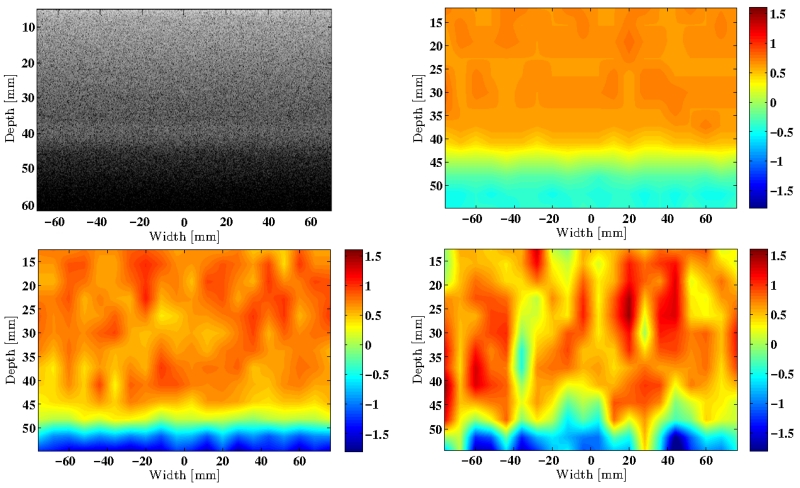
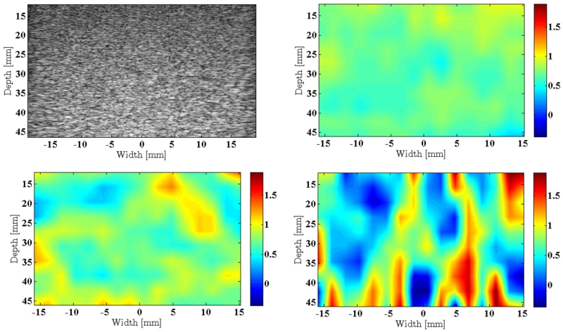
RF data from the simulated phantoms were processed according to the three methods described above, and attenuation coefficient maps were generated. These maps and the B-mode image of the simulated sample phantom (0.7 dB/cm/MHz) are presented in Fig. 1. Since the transmit pulse had a 10 MHz center frequency, the maximum penetration depth of the ultrasound signal was less than the 10 cm depth of the simulated phantom. It was observed, in this case, that the ultrasound signal gets attenuated to levels below the additive white noise at about a depth of 5 cm, and the B-mode image was unresolvable beyond a depth of 6cm. As a result, the visualized depth in Fig. 1 was limited to a range that allows for attenuation estimation. Statistical analysis of the attenuation coefficient estimates was also performed in this depth range, i.e., up to 45mm.

Fig. 1.

B-mode image of the simulated uniform TM phantom with an attenuation coefficient of 0.7 dB/cm/MHz (Upper Left). Estimated attenuation coefficient maps created using the OPSSE (Upper Right), the NPSSE (Lower Left), and the CPSSE (Lower Right).

It is clear from this figure that NPSSE and OPSSE estimate attenuation coefficient with progressively smaller variances compared to CPSSE (i.e., the Hybrid method). Furthermore, unlike the Hybrid method, there were no negative attenuation estimates with these new methods up to the depth of 45 mm. The following plots quantitatively compare the three methods as well as the theoretical expressions derived above.

1) Data Block Length

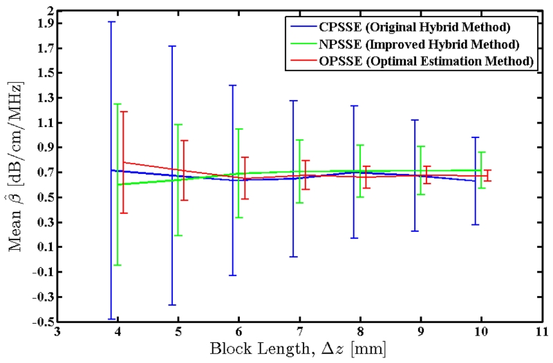
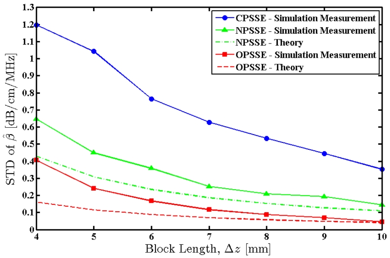
The block length parameter, Δz, was varied from 4 to 10 mm in 1 mm steps. Smaller window lengths do not provide stable power spectral estimates with high enough spectral resolution [26], and larger window lengths do not produce a statistically significant number of attenuation coefficient estimates in this depth range. Attenuation estimation was repeated at each step using the new parameter value, and mean and standard deviation of the estimates were measured for each method. Fig. 2 shows the mean value of the attenuation coefficient estimates, with error bars indicating the observed standard deviation. Fig. 3 shows the measured standard deviations as well as the theoretically predicted standard deviations for the new methods. Note that the new methods proposed in this paper (NPSSE and OPSSE) provide estimates with much lower variance, and without any significant bias.

Fig. 2.

Mean value of the attenuation coefficients estimated over an RF frame of the simulated uniform TM phantom using the three methods. True value of the attenuation coefficient for this phantom is 0.7 dB/cm/MHz. Error bars indicate the observed standard deviations.

Fig. 3.

Standard deviation of the attenuation coefficients estimated over an RF frame of the simulated uniform TM phantom using the three methods. Solid lines indicate measured values and dashed lines indicate theoretically predicted values.

2) Transmit Pulse Bandwidth

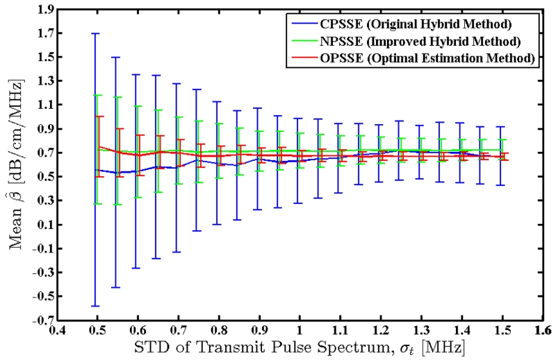
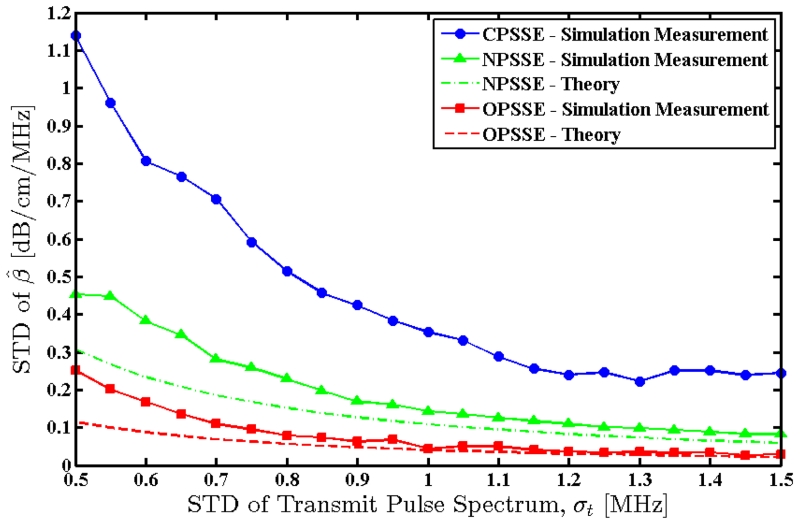
Bandwidth of the transmit pulse (centered at 10 MHz) was varied by changing the standard deviation of its Gaussian spectral form, σ_t, from 0.5 to 1.5 MHz in 50 KHz steps. At each point, RF data acquisition was simulated using the new transmit pulse and the resulting RF frame was processed according to the three methods. Mean and standard deviation of the attenuation coefficient estimates were measured for each method. Fig. 4 shows the mean value of the attenuation coefficient estimates, with error bars indicating the observed standard deviation. Fig. 5 shows the measured standard deviations as well as the theoretically predicted standard deviations for the new methods. Observe that the new methods (NPSSE and OPSSE) provide estimates with considerably lower variance, without any significant bias. However, the Hybrid method (using CPSSE) underestimates the attenuation coefficient at lower bandwidths and exhibits higher estimation variance.

Fig. 4.

Mean value of the attenuation coefficients estimated over an RF frame of the simulated uniform TM phantom using the three methods. True value of the attenuation coefficient for this phantom is 0.7 dB/cm/MHz. Error bars indicate the observed standard deviations.

Fig. 5.

Standard deviation of the attenuation coefficients estimated over an RF frame of the simulated uniform TM phantom using the three methods. Solid lines indicate measured values and dashed lines indicate theoretically predicted values.

3) Number of Data Segments per Block

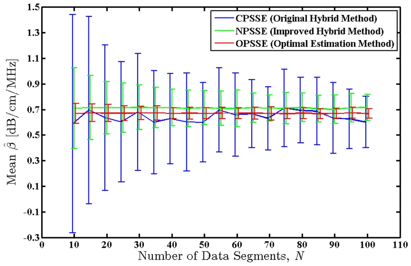
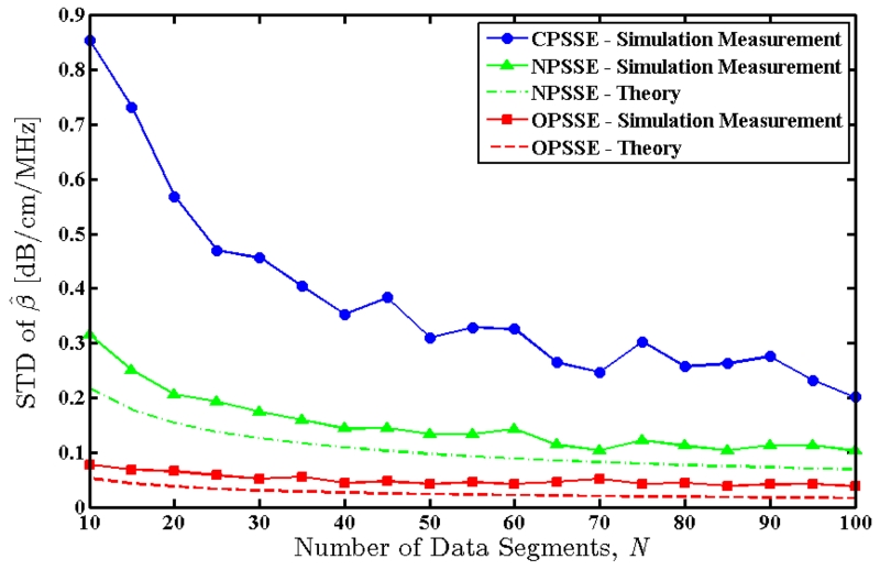
The number of data segments per block, N, was varied by changing the number of adjacent and independent A-lines that are included in each data block from 10 to 100 A-lines in steps of 5. Attenuation estimation was repeated at each step using the new parameter value, and mean and standard deviation of the estimates were measured for each method. Fig. 6 shows the mean value of the attenuation coefficient estimates, with error bars indicating the observed standard deviation. Fig. 7 shows the measured standard deviations as well as the theoretically predicted standard deviations for the new methods. In addition to greatly reduced variance, NPSSE and OPSSE appear to provide a more stable estimation with respect to the variable number of data segments per block. The OPSSE method slightly underestimates the attenuation coefficient when compared to NPSSE in this case.

Fig. 6.

Mean value of the attenuation coefficients estimated over an RF frame of the simulated uniform TM phantom using the three methods. True value of the attenuation coefficient for this phantom is 0.7 dB/cm/MHz. Error bars indicate the observed standard deviations.

Fig. 7.

Standard deviation of the attenuation coefficients estimated over an RF frame of the simulated uniform TM phantom using the three methods. Solid lines indicate measured values and dashed lines indicate theoretically predicted values.

B. Physical TM Phantom Results

Experimentally acquired RF data from the physical phantoms were processed according to the three methods and attenuation coefficient maps were formed. These maps and the B-mode image of the sample phantom (0.8 dB/cm/MHz) are presented in Fig. 8. Similar to the simulated results, NPSSE and OPSSE estimate attenuation coefficient with progressively lower variances when compared to CPSSE (i.e., the Hybrid method). Also, negative attenuation coefficient estimates only appear in the map created using the original Hybrid method. The following plots quantitatively compare the three methods as well as their corresponding theoretical expressions.

Fig. 8.

B-mode image of the physical uniform TM phantom with an attenuation coefficient of 0.8 dB/cm/MHz (Upper Left). Estimated attenuation coefficient maps created using the OPSSE (Upper Right), the NPSSE (Lower Left), and the CPSSE (Lower Right).

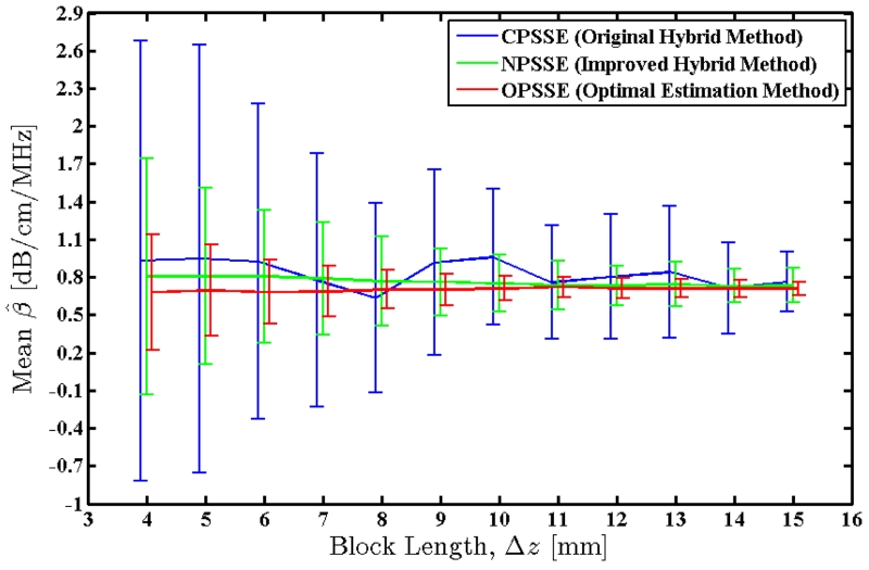
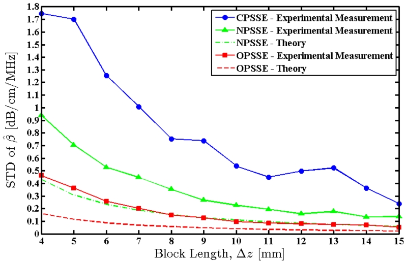
1) Data Block Length

The block length parameter, Δz, was varied from 4 to 15 mm in 1 mm steps. Attenuation estimation was repeated at each step using the new parameter value, and mean and standard deviation of the estimates were measured across the entire frame for each method. Fig. 9 shows the mean value of the attenuation coefficient estimates, with error bars indicating the observed standard deviation. Fig. 10 shows the measured standard deviations as well as the theoretically predicted standard deviations for the new methods. Note that the new methods (NPSSE and OPSSE) provide estimates with lower variance and higher stability compared to the Hybrid method. The OPSSE slightly underestimates the attenuation coefficient for small block lengths, but converges to the true value with longer blocks.

Fig. 9.

Mean value of the attenuation coefficients estimated over an RF frame of the physical uniform TM phantom using the three methods. True value of the attenuation coefficient for this phantom is 0.8 dB/cm/MHz. Error bars indicate the observed standard deviations.

Fig. 10.

Standard deviation of the attenuation coefficients estimated over an RF frame of the physical uniform TM phantom using the three methods. Solid lines indicate measured values and dashed lines indicate theoretically predicted values.

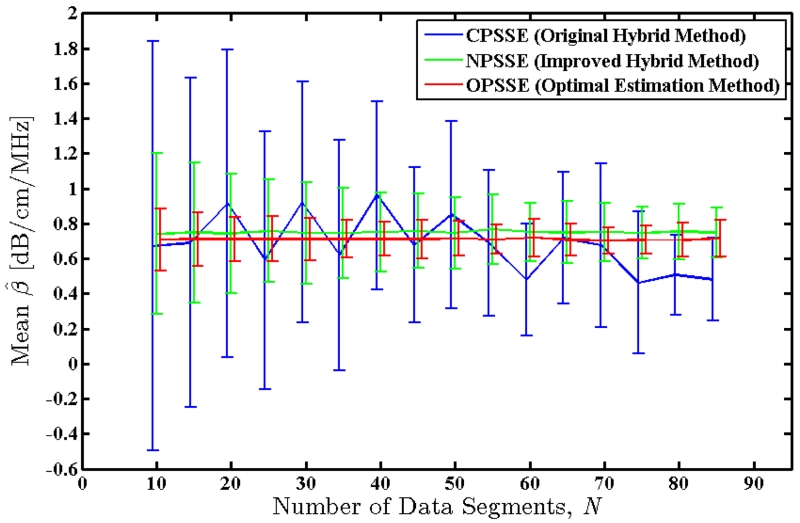
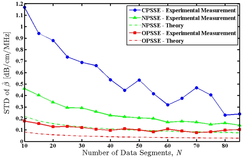
2) Number of Data Segments per Block

The number of data segments per block, N, was varied by changing the number of adjacent and independent A-lines that are included in each data block from 10 to 85 A-lines in steps of 5. A new attenuation coefficient map was estimated at each step using the new parameter value, and mean and standard deviation of the estimates were measured across the entire frame for each method. Fig. 11 shows the mean value of the attenuation coefficient estimates, with error bars indicating the observed standard deviation. Fig. 12 shows the measured standard deviations as well as the theoretically predicted standard deviations for the new methods. Similar to the simulated results, the original Hybrid method provides unstable estimates with respect to the number of data segments per block. NPSSE and OPSSE provide more consistent estimates. However, OPSSE somewhat underestimates the attenuation coefficient.

Fig. 11.

Mean value of the attenuation coefficients estimated over an RF frame of the physical uniform TM phantom using the three methods. True value of the attenuation coefficient for this phantom is 0.8 dB/cm/MHz. Error bars indicate the observed standard deviations.

Fig. 12.

Standard deviation of the attenuation coefficients estimated over an RF frame of the physical uniform TM phantom using the three methods. Solid lines indicate measured values and dashed lines indicate theoretically predicted values.

V. Discussion

The new spectral shift estimators proposed in this paper appear to have significant advantages when compared to the original implementation of the Hybrid method. Namely, they provide greatly reduced estimation variance and increased estimation stability. The theoretical variance expressions derived for OPSSE and NPSSE show acceptable agreement with observed variance in both simulated and experimental data. The only exception is with small data block (i.e., window) lengths, where spectral broadening effects lead to degradation of the assumption that spectral samples are uncorrelated.

Derivation of the theoretical variance expressions for our new methods was performed under the assumption of diffuse scattering conditions, which was used to arrive at (22)-(24). Deviation from diffuse scattering could potentially lead to disagreements between the theoretical expression and observations. However, optimality of the new spectral shift estimator does not depend on a particular probability density function such as the one we assumed for RB(f,z). Rather, it only depends on the mean and variance of the estimated power spectrum and whether they are related in a fashion similar to (4) and (6).

Special care must be taken while implementing the optimum estimator described in this paper. Exponential weights of (28) can lead to arithmetic overflow at far ends of the power spectrum. Therefore, it helps to limit the spectral search band to a frequency range that contains all of the spectral information. Additionally, choice of this search band and its width determines the goodness of agreement between theoretical prediction and observed variance. More specifically, we assumed that a ±3σ_t frequency band contains all of the spectral information and used it to derive (30). Assuming a wider frequency band will drive down the variance predicted by our theoretical expression further, but no experimental improvement will be observed since there is no added spectral information in the wider band. The theoretical expression for variance of the NPSSE, on the other hand, does not shrink with increased search width. Rather, it asymptotically approaches the approximation of (35).

VI. Conclusion

We have introduced an optimum frequency-shift estimator of the attenuation coefficient using a reference phantom, and theoretically demonstrated that it achieves the CRLB. We derived theoretical expressions for estimation variance of this method in terms of processing and system parameters such as window length, number of data segments per block, transmit pulse bandwidth, and number of regression points used per attenuation estimation ROI. Simulated and experimental phantom studies validated the superior performance of this method compared to other prevalent methods. The standard deviation of estimates given by the OPSSE and the NPSSE were observed to be at least 3 and 2 times smaller than that of the Hybrid method, respectively.

Traditional Spectral Shift methods prior to introduction of the Hybrid method were very difficult to implement on array systems, particularly due to diffraction effects that distort the power spectra. Using a reference phantom to correct for diffraction and other system-related effects, the Hybrid method made it possible to generate spectral-shift attenuation maps on clinical array systems. However, the Hybrid method was not stable enough to provide reliable attenuation coefficient images. The reduced estimation variance and near elimination of the negative attenuation coefficient estimates achieved by the optimum estimator of this paper make it possible to realistically pursue mapping of attenuation coefficient as a new ultrasonic imaging modality.

Biographies

Kayvan Samimi received the B.S. degree in Electrical Engineering from the University of Tehran, Iran, in 2009, and the M.S. degree in Electrical Engineering from the University of Wisconsin-Madison, Madison, WI, in 2011, where he is currently a Ph.D. candidate. His research interests are in signal processing applications in medical ultrasound imaging including attenuation estimation, tissue characterization, temperature imaging, and other areas of Quantitative Ultrasound. Mr. Samimi is a student member of IEEE, the American Institute of Ultrasound in Medicine (AIUM), and Eta Kappa Nu.

Tomy Varghese received the B.E. degree in Instrumentation Technology from the University of Mysore, India in 1988, and the M.S. and Ph.D in electrical engineering from the University of Kentucky, Lexington, KY in 1992 and 1995, respectively. From 1988 to 1990 he was employed as an Engineer in Wipro Information Technology Ltd. India. From 1995 to 2000, he was a post-doctoral research associate at the Ultrasonics laboratory, Department of Radiology, University of Texas Medical School, Houston, TX. He joined the Department of Medical Physics at the University of Wisconsin-Madison, Madison, WI in 2000 as an Assistant Professor. He is currently a Professor in the same department. His research interests include elastography, ultrasound imaging, Quantitative ultrasound, detection and estimation theory, statistical pattern recognition and signal and image processing applications in medical imaging. Dr. Varghese is a fellow of the American Institute of Ultrasound in Medicine (AIUM), senior member of the IEEE, and a member of the American Association of Physicists in Medicine (AAPM) and Eta Kappa Nu.

References

- [1].Oelze ML, O’Brien WD., Jr Frequency-dependent attenuation-compensation functions for ultrasonic signals backscattered from random media. J. Acoust. Soc. Am. 2002;111(5):2308–2319. doi: 10.1121/1.1452743. [DOI] [PubMed] [Google Scholar]
- [2].Nam K, Rosado-Mendez IM, Wirtzfeld LA, Ghoshal G, Pawlicki AD, Madsen EL, Lavarello RJ, Oelze ML, Zagzebski JA, O’Brien WD, Jr, Hall TJ. Comparison of ultrasound attenuation and backscatter estimates in layered tissue-mimicking phantoms among three clinical scanners. Ultrason. Imaging. 2012;34(4):209–221. doi: 10.1177/0161734612464451. [DOI] [PMC free article] [PubMed] [Google Scholar]
- [3].Gaitini D, Baruch Y, Ghersin E, Veitsman E, Kerner H, Shalem B, Yaniv G, Sarfaty C, Azhari H. Feasibility study of ultrasonic fatty liver biopsy: texture vs. attenuation and backscatter. Ultrasound Med. Biol. 2004;30(10):1321–1327. doi: 10.1016/j.ultrasmedbio.2004.08.001. [DOI] [PubMed] [Google Scholar]
- [4].Ghoshal G, Lavarello RJ, Kemmerer JP, Miller RJ, Oelze ML. Ex vivo Study of Quantitative Ultrasound Parameters in Fatty Rabbit Livers. Ultrasound Med. Biol. 2012;38(12):2238–2248. doi: 10.1016/j.ultrasmedbio.2012.08.010. [DOI] [PMC free article] [PubMed] [Google Scholar]
- [5].Narayana PA, Ophir J. On the frequency dependence of attenuation in normal and fatty liver. IEEE Trans. Sonics Ultrason. 1983;30(6):379–383. [Google Scholar]
- [6].Lin T, Ophir J, Potter G. Correlation of ultrasonic attenuation with pathologic fat and fibrosis in liver disease. Ultrasound Med. Biol. 1988;14(8):729–734. doi: 10.1016/0301-5629(88)90028-2. [DOI] [PubMed] [Google Scholar]
- [7].Kuc R. Clinical application of an ultrasound attenuation coefficient estimation technique for liver pathology characterization. IEEE Trans. Biomed. Eng. 1980;6:312–319. doi: 10.1109/TBME.1980.326739. [DOI] [PubMed] [Google Scholar]
- [8].Chang CH, Huang SW, Yang HC, Chou YH, Li PC. Reconstruction of ultrasonic sound velocity and attenuation coefficient using linear arrays: Clinical assessment. Ultrasound Med. Biol. 2007;33(11):1681–1687. doi: 10.1016/j.ultrasmedbio.2007.05.012. [DOI] [PubMed] [Google Scholar]
- [9].D’Astous F, Foster F. Frequency dependence of ultrasound attenuation and backscatter in breast tissue. Ultrasound Med. Biol. 1986;12(10):795–808. doi: 10.1016/0301-5629(86)90077-3. [DOI] [PubMed] [Google Scholar]
- [10].Mimbs JW, Yuhas D, Miller J, Weiss AN, Sobel BE. Detection of myocardial infarction in vitro based on altered attenuation of ultrasound. Circulation Research. 1977;41(2):192–198. doi: 10.1161/01.res.41.2.192. [DOI] [PubMed] [Google Scholar]
- [11].O’Donnell M, Mimbs J, Miller J. Relationship between collagen and ultrasonic backscatter in myocardial tissue. J. Acoust. Soc. Am. 1981;69(2):580–588. doi: 10.1121/1.385433. [DOI] [PubMed] [Google Scholar]
- [12].Baldwin SL, Marutyan KR, Yang M, Wallace KD, Holland MR, Miller JG. Estimating myocardial attenuation from M-mode ultrasonic backscatter. Ultrasound Med. Biol. 2005;31(4):477–484. doi: 10.1016/j.ultrasmedbio.2004.12.024. [DOI] [PubMed] [Google Scholar]
- [13].Shi H, Varghese T, Dempsey RJ, Salamat MS, Zagzebski JA. Relationship Between Ultrasonic Attenuation, Size and Axial Strain Parameters for Ex Vivo Atherosclerotic Carotid Plaque. Ultrasound Med. Biol. 2008;34(10):1666–1677. doi: 10.1016/j.ultrasmedbio.2008.02.014. [DOI] [PMC free article] [PubMed] [Google Scholar]
- [14].Shi H, Varghese T, Mitchell CC, McCormick M, Dempsey RJ, Kliewer MA. In vivo attenuation and equivalent scatterer size parameters for atherosclerotic carotid plaque: Preliminary results. Ultrasonics. 2009;49(8):779–785. doi: 10.1016/j.ultras.2009.06.004. [DOI] [PMC free article] [PubMed] [Google Scholar]
- [15].Bridal SL, Beyssen B, Fornès P, Julia P, Berger G. Multiparametric attenuation and backscatter images for characterization of carotid plaque. Ultrason. Imaging. 2000;22(1):20–34. doi: 10.1177/016173460002200102. [DOI] [PubMed] [Google Scholar]
- [16].Wear KA. Ultrasonic attenuation in human calcaneus from 0.2 to 1.7 MHz. IEEE Trans. Ultrason. Ferroelectr. Freq. Control. 2001;48(2):602–608. doi: 10.1109/58.911743. [DOI] [PMC free article] [PubMed] [Google Scholar]
- [17].Wear KA. Frequency dependence of ultrasonic backscatter from human trabecular bone: Theory and experiment. J. Acoust. Soc. Am. 1999;106(6):3659–3664. doi: 10.1121/1.428218. [DOI] [PMC free article] [PubMed] [Google Scholar]
- [18].François T, Cloutier G. Experimental ultrasound characterization of red blood cell aggregation using the structure factor size estimator. J. Acoust. Soc. Am. 2007;122(1):645–656. doi: 10.1121/1.2735805. [DOI] [PubMed] [Google Scholar]
- [19].Franceschini E, François T, Destrempes F, Cloutier G. Ultrasound characterization of red blood cell aggregation with intervening attenuating tissue-mimicking phantoms. J. Acoust. Soc. Am. 2010;127(2):1104–1115. doi: 10.1121/1.3277200. [DOI] [PMC free article] [PubMed] [Google Scholar]
- [20].Kuc R, Schwartz M. Estimating the acoustic attenuation coefficient slope for liver from reflected ultrasound signals. IEEE Trans. Sonics Ultrason. 1979;26(5):353–361. [Google Scholar]
- [21].Wilson LS, Robinson DE, Doust BD. Frequency domain processing for ultrasonic attenuation measurement in liver. Ultrason Imaging. 1984;6(3):278–292. doi: 10.1177/016173468400600303. [DOI] [PubMed] [Google Scholar]
- [22].Fink M, Hottier F, Cardoso J. Ultrasonic signal processing for in vivo attenuation measurement: short time Fourier analysis. Ultrason. Imaging. 1983;5(2):117–135. doi: 10.1177/016173468300500202. [DOI] [PubMed] [Google Scholar]
- [23].Samimi K, Varghese T. Performance evaluation of the spectral centroid downshift method for attenuation estimation. IEEE Trans. Ultrason. Ferroelectr. Freq. Control. 2015;62(5):871–880. doi: 10.1109/TUFFC.2014.006945. [DOI] [PMC free article] [PubMed] [Google Scholar]
- [24].Laugier P, Berger G, Fink M, Perrin J. Diffraction correction for focused transducers in attenuation measurements in vivo. Ultrason. Imaging. 1987;9(4):248–259. doi: 10.1177/016173468700900403. [DOI] [PubMed] [Google Scholar]
- [25].Kim H, Varghese T. Attenuation estimation using spectral cross-correlation. IEEE Trans. Ultrason. Ferroelectr. Freq. Control. 2007;54(3):510–519. doi: 10.1109/tuffc.2007.274. [DOI] [PubMed] [Google Scholar]
- [26].Yao LX, Zagzebski JA, Madsen EL. Backscatter coefficient measurements using a reference phantom to extract depth-dependent instrumentation factors. Ultrason. Imaging. 1990;12(1):58–70. doi: 10.1177/016173469001200105. [DOI] [PubMed] [Google Scholar]
- [27].Kim H, Varghese T. Hybrid spectral domain method for attenuation slope estimation. Ultrasound Med. Biol. 2008;34(11):1808–1819. doi: 10.1016/j.ultrasmedbio.2008.04.011. [DOI] [PubMed] [Google Scholar]
- [28].Rosado-Mendez IM, Nam K, Hall TJ, Zagzebski JA. Task-oriented comparison of power spectral density estimation methods for quantifying acoustic attenuation in diagnostic ultrasound using a reference phantom method. Ultrason. Imaging. 2013;35(3):214–234. doi: 10.1177/0161734613495524. [DOI] [PMC free article] [PubMed] [Google Scholar]
- [29].Kuc R. Estimating acoustic attenuation from reflected ultrasound signals: comparison of spectral-shift and spectral-difference approaches. IEEE Trans. Acoust. Speech. 1984;32(1):1–6. [Google Scholar]
- [30].Bamler R. Doppler frequency estimation and the Cramer-Rao bound. IEEE Trans. Geosci. Remote Sens. 1991;29(3):385–390. [Google Scholar]
- [31].Labyed Y, Bigelow TA. A theoretical comparison of attenuation measurement techniques from backscattered ultrasound echoes. J. Acoust. Soc. Am. 2011;129(4):2316–2324. doi: 10.1121/1.3559677. [DOI] [PMC free article] [PubMed] [Google Scholar]
- [32].Omari EA, Varghese T. Signal to noise ratio comparisons for ultrasound attenuation slope estimation algorithms. Med. Phys. 2014;41(3):032902. doi: 10.1118/1.4865781. [DOI] [PMC free article] [PubMed] [Google Scholar]
- [33].Papoulis A, Pillai SU. Probability, Random Variables, and Stochastic Processes. McGraw-Hill; New York, NY, USA: 2002. ch.4: The concept of a random variable. [Google Scholar]
- [34].Kay SM. Fundamentals of Statistical Signal Processing: Estimation Theory. Prentice Hall PTR; Upper Saddle River, NJ, USA: 1993. ch.3: Cramer-Rao lower bound. [Google Scholar]
- [35].Wagner RF, Smith SW, Sandrik JM, Lopez H. Statistics of speckle in ultrasound B-scans. IEEE Trans. Sonics Ultrason. 1983;30(3):156–163. [Google Scholar]
- [36].Wagner RF, Insana MF, Brown DG. Statistical properties of radio-frequency and envelope-detected signals with applications to medical ultrasound. J. Opt. Soc. Am. A. 1987;4(5):910–922. doi: 10.1364/josaa.4.000910. [DOI] [PMC free article] [PubMed] [Google Scholar]
- [37].Chaturvedi P, Insana MF. Error bounds on ultrasonic scatterer size estimates. J. Acoust. Soc. Am. 1996;100(1):392–399. doi: 10.1121/1.415958. [DOI] [PubMed] [Google Scholar]
- [38].Chen Q. Computer simulations in parametric ultrasonic imaging. University of Wisconsin-Madison; Ann Arbor: ProQuest/UMI: 2004. PhD dissertation. Publication No. AAI3127983. [Google Scholar]
- [39].Welch PD. The use of fast Fourier transform for the estimation of power spectra: a method based on time averaging over short, modified periodograms. IEEE Trans. Audio. 1967;15:70–73. [Google Scholar]