Empirical Bayes Estimation of Coalescence Times from Nucleotide Sequence Data

Abstract

We demonstrate the advantages of using information at many unlinked loci to better calibrate estimates of the time to the most recent common ancestor (TMRCA) at a given locus. To this end, we apply a simple empirical Bayes method to estimate the TMRCA. This method is both asymptotically optimal, in the sense that the estimator converges to the true value when the number of unlinked loci for which we have information is large, and has the advantage of not making any assumptions about demographic history. The algorithm works as follows: we first split the sample at each locus into inferred left and right clades to obtain many estimates of the TMRCA, which we can average to obtain an initial estimate of the TMRCA. We then use nucleotide sequence data from other unlinked loci to form an empirical distribution that we can use to improve this initial estimate.

WITHOUT intralocus recombination, all DNA sequences sampled at a given genetic locus originate from a common ancestor. That is, if we follow the genetic lineages of these sequences back in time, they will merge with one another until a single inheritance path remains. For each locus, this process yields a genealogical tree that unites all of the sampled sequences. The time to the most recent common ancestor (TMRCA) of a particular locus is the height of the genealogical tree at that locus.

TMRCA estimates are commonly used in inferring demographic history. For example, the TMRCA can be used to place an upper bound on the divergence time of subpopulations, if the migration rate between subpopulations and the size of each subpopulation are relatively small (Rosenberg and Feldman 2002). This idea has been applied to obtain the evolutionary history of a number of different organisms, from chaffinches to anchovies (Griswold and Baker 2002; Hailer et al. 2012).

Early articles in the TMRCA literature studied the human mitochondrial DNA ancestor, which supported the African origin hypothesis (Vigilant et al. 1991). Later studies sought to infer the TMRCA of the Y chromosome, to shed light on the origin and dispersal of modern humans. This was challenging due to the scarcity of DNA sequence polymorphisms on the Y chromosome (Jakubiczka et al. 1989; Hammer 1995). One early study examined the Zfy intron, which was revealed to be completely monomorphic in a sample of 38 males (Dorit et al. 1995). Estimating the TMRCA of this intron necessitated a Bayesian approach, because any estimate proportional to the number of mutations would have given a value of zero. Dorit et al. (1995) used a uniform prior distribution on the TMRCA, which was considered inappropriate by a number of commenters, who advocated using priors that stemmed from coalescent theory and their preferred demographic models (Donnelly et al. 1996; Fu and Li 1996; Weiss and von Haeseler 1996). As a result of the lack of signal in the data, these different studies inferred very different estimates of the TMRCA (Brookfield 1997). Further efforts to infer the TMRCA for other Y chromosome data have also been affected by this dependence on the prior (Hammer 1995; Whitfield et al. 1995; Walsh 2001).

Given the interest in the TMRCA of an individual gene in inferring demography, the dependence of the estimate on the prior demographic model is particularly problematic (Brookfield 1997). In contrast to parametric Bayesian methods such as those applied to Y chromosome data, frequentist approaches such as maximum likelihood do not require the specification of a prior and so might appear preferable. One such frequentist estimator is the one proposed by Tang et al. (2002). In this method, nucleotide sequence data are used to partition the sample into two groups, corresponding to the inferred two clades on either side of the root of the tree. Tang et al. (2002) then estimate the TMRCA, using the average number of nucleotide sequence differences across all left–right clade pairs, $D_i.$

Of course, application of this method to the Zfy data would give an estimate of zero for the TMRCA, which is a clear underprediction. More generally, if Tang et al. (2002) had regressed true TMRCA on estimated TMRCA, it would have been revealed that their method tends to underpredict when the number of segregating sites at a locus is small and to overpredict when it is large. This is because an extreme number of segregating sites at a locus often results from a combination of a relatively small or large TMRCA at that locus and a relatively small or large number of mutations conditional on the TMRCA. Errors in inference will occur if all of the variation in the number of segregating sites is attributed to variation in times to most recent common ancestry, as is the case generally in frequentist approaches.

We propose augmenting the method of Tang et al. (2002) by using information at unlinked loci to better calibrate estimates of the TMRCA, and we introduce a very simple nonparametric empirical Bayes method. By “nonparametric,” we mean that we do not assume that the prior on the TMRCA has any particular shape, only that all loci’s TMRCAs are sampled from the same distribution. In addition to improving on Tang et al. (2002)’s estimator, our method is advantageous over many Bayesian methods in that it makes no prior assumptions about the distribution of TMRCAs and therefore can be used when the history of the population is completely unknown. We show that our method performs well in simulated data from a wide variety of demographic scenarios.

The idea of using information at additional loci to improve the estimate at one locus appears in a number of recent methods, e.g., Hobolth et al. (2007) and Li and Durbin (2011), although mostly with a spatial context along the genome that our method does not have. Similarly to Li and Durbin (2011), our method is able to extract information from a single genome, by making use of the number of heterozygote sites in sequences of DNA between recombination break points. We apply this method to a single Bantu individual and a single European individual and are able to show that loci with the same number of heterozygous sites in different populations have different average TMRCAs.

Materials and Methods

Assumptions

We assume that the number of mutations at a locus follows a Poisson distribution with constant rate equal to the product of the total genealogical branch length and the per locus mutation rate. In addition, we assume that each mutation generates a new segregating site, in accordance with the infinite-sites model developed by Watterson (1975), which also includes the assumption of complete linkage among sites at a locus. In fact, we allow for the possibility of within-locus recombination as long as it does not modify tree topology or TMRCA, which would preclude the application of Tang et al. (2002)’s method. Finally, we assume that all of the different loci under consideration are independent, in the sense that they represent independent samples from the distribution of TMRCA. Approximate independence can be achieved by allowing for sufficient interlocus distance.

Simple existing methods for inferring the TMRCA of a sampled pair

Let us first consider estimating the TMRCA at a locus i in a sample of size 2. The number of nucleotide differences $x_i$ between these two samples follows a Poisson distribution with rate $2{\mu }_i{\ell }_i{T}_i,$ where ${\mu }_i$ is the per nucleotide mutation rate at that locus, ${\ell }_i$ is the length of the sequenced region, and $T_i$ is the time until coalescence measured in coalescent units. One natural estimator of $T_i$ is the maximum-likelihood estimator, used for example by Tang et al. (2002):

$${\widehat{T}}_{i,\mathrm{Freq}}\mathrm{=}\frac{D_i}{2{\mu }_i{\ell }_i}.$$ (1)

In Tang et al. (2002), $D_i$ is the average number of segregating sites across all left–right clade pairs, and for $n=2,$ $D_i=x_i.$

Within the framework of coalescent theory, where priors for $T_i$ have been derived for a number of demographic models, it is more common to estimate $T_i$ using a parametric Bayesian approach. However, this requires certain assumptions about demographic history, which we might ideally prefer not to make. One such estimator is the posterior mean, which can be obtained in the manner of equations 19 and 20 in Tajima (1983) for an exponential prior on the TMRCA, which corresponds to the demographic assumption of a constant population size,

$${\widehat{T}}_{i,\text{Bayes}}=\frac{\theta }{\left(1+\theta \right)}\frac{x_i+1}{2{\mu }_i{\ell }_i},$$ (2)

where $\theta =4N_{\mathrm{e}}{\mu }_i{\ell }_i,$ and $N_{\mathrm{e}}$ is the effective population size.

Nonparametric empirical Bayes approach

We can use Robbins’ (1955) method to improve on these simple frequentist and parametric Bayesian approaches, by utilizing information from other unlinked loci in the sample. Robbins considered the following case of sampling from a mixed distribution. Let $x_i,$ conditional on some variable $T_i,$ be specified by a Poisson distribution,

$$P\left(x_i|T_i\right)=\frac{T_i^{x_i}{e}^{-T_i}}{x_i\mathrm{!}}.$$

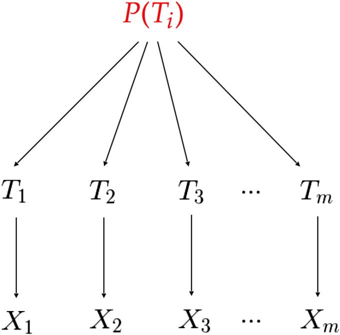
The $T_i$ are in turn independent and identically distributed according to some distribution, which we do not know and do not need to specify. For an illustration of the data-generating process, see Figure 1.

Figure 1.

Data-generating process for Robbins’ (1955) method, in which the distribution $P\left(T_i\right)$ is unknown and does not need to be specified.

This data-generating process exactly describes the process that yields the number of mutations at unlinked loci in a genome, given our assumptions. That is, conditional on $T_i$ and ${\mu }_i{\ell }_i,$ each $X_i$ is an independently distributed Poisson random variable with rate $2{\mu }_i{\ell }_i{T}_i,$ and each $T_i$ is drawn i.i.d. from an unknown distribution. For the sake of computational simplicity, we assume that $2{\mu }_i{\ell }_i=1,$ which is equivalent to a simple rescaling of $T_i.$

Under this compound sampling scheme (although initially not applied to genetic data), Robbins (1955) showed that we can obtain a point estimate of $T_i$ by making use of Bayes’ rule and the form of the Poisson probability distribution,

$$\begin{array}{c}E\left[T_i|X_i=x_i\right]={\displaystyle \int T_{i}P\left(T_i|x_i\right)d{T}_i}\\ ={\displaystyle \int T_i\frac{P\left(x_i|T_i\right)P\left(T_i\right)}{P\left(x_i\right)}d{T}_i}\\ =\frac{\left(x_i+1\right)}{P\left(x_i\right)}{\displaystyle \int \frac{e^{-T_i}{T}_i^{x_i+1}}{\left(x_i+1\right)\mathrm{!}}P\left(T_i\right)d{T}_i}\\ =\frac{\left(x_i+1\right)}{P\left(x_i\right)}{\displaystyle \int P\left(x_i+1|T_i\right)P\left(T_i\right)d{T}_i}=\frac{\left(x_i+1\right)P\left(x_i+1\right)}{P\left(x_i\right)},\end{array}$$

where $P\left(x_i\right)$ is the marginal probability that $X_i=x_i,$ that is, the marginal probability that we observed exactly $x_i$ segregating sites at locus i. As can be seen from the sampling structure depicted in Figure 1, this marginal distribution, which we could simply call $P\left(x\right),$ does not depend on i.

When the number of loci is not too small, we can approximate $P\left(x_i\right)$ by the fraction of loci where the number of observed segregating sites is equal to $x_i.$ We use $m_{x_i}$ to refer to m times this fraction or the number of loci with exactly $x_i$ mutations. In this way we obtain the following estimator of the TMRCA at locus i,

$${\widehat{T}}_{i,\mathrm{NPEB}}=\left(x_i+1\right)\frac{m_{x_i+1}}{m_{x_i}},$$ (3)

where NPEB is the nonparametric empirical Bayes approach. Note that mutation rates vary across the genome, and we are not assuming a single underlying mutation rate. Loci with relatively high mutation rates, for example, can be truncated, such that the product of the mutation rate and the locus length ${\mu }_i{\ell }_i$ across all considered loci is roughly similar.

Robbins (1955) proved that this estimator is asymptotically optimal. That is, as the total number of loci sampled grows ($\mathit{m}\mathrm{\to \infty }$), its Bayes risk (such as the mean squared error) converges to the Bayes risk for the Bayesian model where the true prior of the $T_i,$ and therefore $\mathit{P}\left(x_i\right),$ is known. As might be expected, Robbins’ (1955) method behaves erratically in cases where there are few data. If, for example, $m_{x_i+1}=0,$ that is if no loci have exactly $x_i+1$ segregating sites, then our estimate of $T_i$ corresponding to a locus i where there are $x_i>0$ segregating sites would be 0, which is clearly wrong. To mitigate this effect, there are a number of smoothing techniques one might apply (Lidstone 1920; Good 1953; Gale and Church 1990, 1994). In this article, we attempt to estimate $T_i$ using Robbins’ (1955) method only when loci where there are $x_i$ segregating sites and loci where there are $x_i+1$ segregating sites are not rare. It is indeed for these loci that Robbins’ (1955) method shows a clear advantage over traditional methods that do not incorporate information from other independent loci.

Another consequence of variation in $m_{x_i}$ is that estimates of $T_i$ are not necessarily a nondecreasing function of the number of mutations $x_i.$ In fact, we would expect loci in which there are more mutations to be at least as ancient as loci in which there are only a few. To remedy this, we can fit a weighted isotonic regression of the inferred mean ${\widehat{T}}_{i,\mathrm{NPEB}}$ on the number of mutations, using the pava( ) function in the “Iso” package (Turner 2015) in R (R Core Team 2015), where we weight each value by

$${\left(x_i+1\right)}^2\frac{m_{x_i+1}^2}{m_{x_i}^2}\left(\frac{1}{m_{x_i}}+\frac{1}{m_{x_i+1}}\right),$$ (4)

and obtain a new set of estimators, denoted by ${\widehat{T}}_{i,\mathrm{NPEB}}^{\mathrm{W}}.$ We use these weights as an approximation of the variance of ${\widehat{T}}_{i,\mathrm{NPEB}},$ as is explained in the Effectiveness of Robbins’ method section. As the isotonic regression yields the least-squares best fit among nondecreasing relationships, performing this step ensures that ${\widehat{\mathit{T}}}_{\mathit{i}}\mathrm{\le }{\widehat{\mathit{T}}}_{\mathit{j}}$ if there are fewer mutations at locus i than at locus j.

To summarize, Robbins’ (1955) method uses the ratio of the number of loci with exactly $x_i$ and $x_i+1$ mutations to calibrate the TMRCA at a given locus with exactly $x_i$ mutations. We then incorporate the knowledge that the expected number of segregating sites at a locus is a nondecreasing function of its TMRCA, by running an isotonic regression on the TMRCA estimates.

Generalizing our estimator to a sample of size $n\ge 2$

In generalizing our estimator for use on samples of size $n\ge 2,$ we are inspired by the frequentist estimation of coalescence times from nucleotide sequence data, using a tree-based partition in Tang et al. (2002). In that work, the n sequences are first partitioned into two subsets that are meant to correspond to the left and right clades of the genealogical tree. The MRCA of any two sequences, one in the left clade and one in the right clade, is the root of the tree. Tang et al. (2002) propose an estimator of the TMRCA based on the average number of pairwise differences $D_i$ between sequences in the left clade and sequences in the right clade (see Equation 1).

Although genealogical trees are not always completely resolved by the data, in many cases there is little ambiguity about the branching pattern at the root (Tang et al. 2002). When ambiguity does exist at the root, Tang et al. (2002) propose a partition algorithm that is less biased than forcing the pair of sequences that differ most from each other to be in different clades. This algorithm does not require knowledge of the ancestral state at the segregating sites. The eight steps of this algorithm are described in detail in Tang et al. (2002).

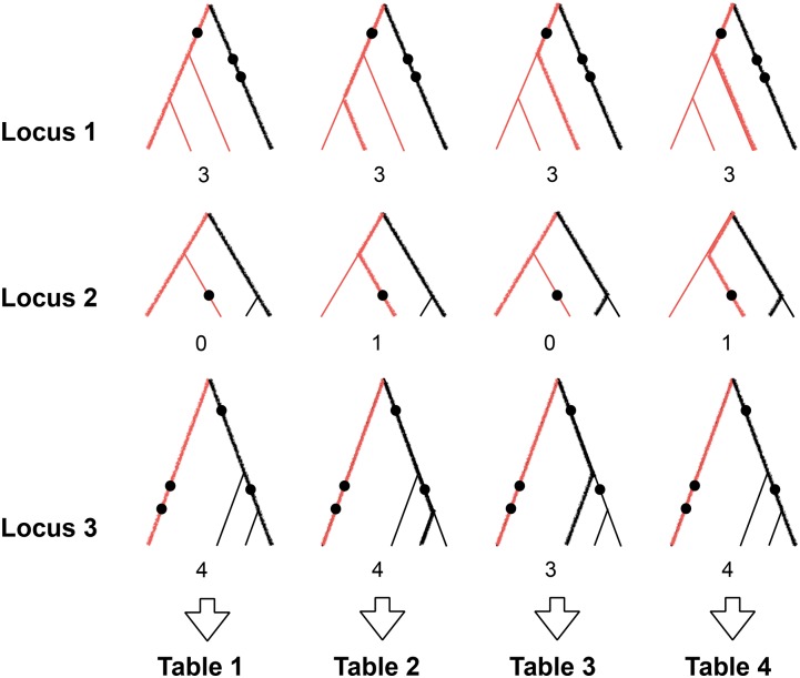
We use the following steps to infer $T_i$ in cases where $n>2,$ which we also illustrate in Figure 2.

Figure 2.

Inferring $T_i$ for $n\ge 2.$ Here we illustrate the particular case where $n=4$ and $m=3.$ Steps 1 and 2 focus on the leftmost column. In step 1, we partition each locus into left and right clades, based on Tang’s algorithm. Left-clades lineages are depicted in red, and right-clade lineages are depicted in black. In step 2, we consider a single random left-clade member and a single random right-clade member at each locus. We represent these with thick lines and count the number of pairwise differences (mutations are represented by black circles), which we write below each tree. In our example, the number of pairwise differences at each locus is (3, 0, 4). We use this information to calculate an estimate of $T_i$ for each unique number of segregating sites, which we store in table 1. In step 3, we repeat this for all left–right pairs. As there are four left–right clade pairs at locus 2, we resample an extra left-clade–right-clade pair at loci 1 and 3, which corresponds to the fourth column. In step 4, we average the TMRCA estimates in all four tables to obtain a final table, again linking different numbers of segregating sites to different estimates of TMRCA. Finally, in step 5, we calculate the average number of pairwise differences between inferred left and right clades at each locus. In our case, this is $\left(D_1,D_2,D_3\right)=\left(3,\hspace{0.17em}0.5,\hspace{0.17em}3.67\right).$ The estimate at locus 3 for example will be 0.67 times the estimate at a locus with four mutations and 0.33 times the estimate at a locus with three mutations.

1. For each locus i, where $1\le i\le m,$ we use Tang et al.’s (2002) tree partitioning algorithm to partition the sample at locus i into left and right clades.

2. From the set of left-clade samples, we pick at random a single sample. We also pick at random a sample from the set of right-clade samples. We calculate the number of pairwise differences and repeat this process for every locus i. The reason we count the number of differences between single pairs of left–right clade sequences instead of averaging the number of differences across all left–right clade pairs is that Robbins’ (1955) method requires $x_i$ to be an integer. We then calculate a ${\widehat{T}}_{i,\mathrm{NPEB}}$ for each locus, using these counts at all m loci, according to Equation 3. The result of this step is a table that contains estimates of TMRCA corresponding to different observed numbers of segregating sites. We then fit a weighted isotonic regression to these estimates, where each estimate is weighted according to Equation 4.

3. Clearly, at the end of the previous step, we have not used much of the information from our sample, as we have sampled only one left-clade–right-clade pair from each locus. We therefore repeat the previous step over all possible left–right clade pairs at a particular locus, which all have the same TMRCA if the partitioning algorithm is correct. For each locus, the number of possible left–right clade pairs depends on the topology of the tree at that locus. If a single sequence forms one of the clades, the data at that locus will consist of $n-1$ highly correlated pairwise differences. When the tree is balanced, there are $\left(n\mathrm{+1}\left(n\hspace{0.17em}\text{is}\hspace{0.17em}\text{odd}\right)\right)\left(n-1\left(n\hspace{0.17em}\text{is}\hspace{0.17em}\text{odd}\right)\right)/4$ pairs, many more than in the unbalanced case. We repeat step 2 until all left-right clade pairs have been used at least once. For loci with the maximum observed number of pairs, each pair is used exactly once. For loci with fewer pairs, some pairs are used multiple times; these are sampled uniformly at random after all pairs at a locus have been used once. At the end of this step, we obtain between $n-1$ and $\left(n+1\left(n\hspace{0.17em}\text{is}\hspace{0.17em}\text{odd}\right)\right)\left(n-1\left(n\hspace{0.17em}\text{is}\hspace{0.17em}\text{odd}\right)\right)/4$ tables, depending on the m inferred tree configurations. That is, the number of tables produced is equal to the number of pairs in the locus with the largest amount of left–right pairs.

4. We average the entries in all of the tables obtained in the previous two steps, i.e., the estimates of TMRCA for each observed number of segregating sites at a locus, and in this way we obtain a final table with the aggregate information that links each integer-valued unique number of segregating sites to a unique estimate of the TMRCA.

5. We then consider the data at a single locus i. We calculate $D_i,$ the average number of segregating sites over all left–right clade pairs at this locus. If this average is an integer, then the estimate of the TMRCA can be read from the row corresponding to value $D_i$ in the final table. More likely than not, though, $D_i$ is not an integer. We can create a piecewise linear function that extends our estimates of the TMRCA to noninteger values of $D_i.$ Our estimate of the TMRCA is then a weighted average of the estimates of the TMRCA in the rows corresponding to $\lfloor D_i\rfloor$ and $\lceil D_i\rceil .$

We note here that the presence of recombination does not compromise the method in any way when $n=2$ but does require a reinterpretation of the meaning of the results. The NPEB estimate will no longer correspond to a single TMRCA at a given locus but to an average TMRCA across the locus. This is due to the additive properties of the Poisson distribution and to the fact that, in a sample of size 2, intralocus recombination will not produce a new tree with a different shape. Indeed, in a sample of size 2, there is no ambiguity concerning the members of the left and the right clades. For a sample size >2, we require no intralocus recombination that affects tree shape, because otherwise we could not partition our sample into left and right clades.

Data availability

The programs sufficient to reproduce the results in this article are available at wakeleylab.oeb.harvard.edu/resources.

Results

Effectiveness of Robbins’ method

To assess where Robbins’ (1955) NPEB method is most effective, we calculate the variance of ${\widehat{T}}_{i,\mathrm{NPEB}}$ as a function of m, $m_{x_i},$ and $m_{x_i+1}.$ Using a Taylor expansion, we can approximate the variance of the ratio of two random variables (Rice 2007):

$$\mathrm{Var}\left(\frac{m_{x_i+1}}{m_{x_i}}\right)\approx \frac{{\left(E\left(m_{x_i+1}\right)\right)}^2}{{\left(E\left(m_{x_i}\right)\right)}^2}\left(\frac{\mathrm{Var}\left(m_{x_i+1}\right)}{{\left(E\left(m_{x_i+1}\right)\right)}^2}-2\frac{\mathrm{Cov}\left(m_{x_i},m_{x_i+1}\right)}{E\left(m_{x_i}\right)E\left(m_{x_i+1}\right)}+\frac{\mathrm{Var}\left(m_{x_i}\right)}{{\left(E\left(m_{x_i}\right)\right)}^2}\right).$$ (5)

We can represent the distribution of the $m_{x_i}$ for each observed $x_i$ by a multinomial distribution, as long as we create a bin to account for all unobserved yet possible values of $x_i.$ In the model there are countably infinite possible numbers of segregating sites, but in practice the number is limited by ${\ell }_i,$ the length in nucleotides of each locus i. By the properties of the multinomial, we have $E\left(m_{x_i}\right)=mP\left(x_i\right),$ $\mathrm{Var}\left(m_{x_i}\right)=mP\left(x_i\right)\left(1-P\left(x_i\right)\right),$ and $\mathrm{Cov}\left(m_{x_i},m_{x_i+1}\right)=-mP\left(x_i\right)P\left(x_i+1\right).$ Equation 5 then simplifies to

$$\mathrm{Var}\left(\frac{m_{x_i+1}}{m_{x_i}}\right)\mathrm{\approx }\frac{P{\left(x_i+1\right)}^2}{mP{\left(x_i\right)}^2}\left(\frac{1}{P\left(x_i\right)}+\frac{1}{P\left(x_i+1\right)}\right).$$

Therefore, as ${\widehat{T}}_{i,\mathrm{NPEB}}=\left(x_i+1\right)\left(m_{x_i+1}/m_{x_i}\right),$ we have

$$\mathrm{Var}\left({\widehat{T}}_{i,\mathrm{NPEB}}\right)=\mathrm{Var}\left(\left(x_i+1\right)\frac{m_{x_i+1}}{m_{x_i}}\right)\approx {\left(x_i+1\right)}^2\frac{P{\left(x_i+1\right)}^2}{mP{\left(x_i\right)}^2}\left(\frac{1}{P\left(x_i+1\right)}+\frac{1}{P\left(x_i\right)}\right).$$ (6)

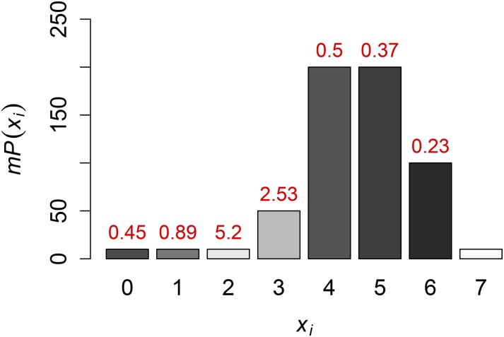
To illustrate where Robbins’ (1955) method is most effective, we apply 6 to each value $x_i$ of an example distribution illustrated in Figure 3. As one might expect, if we increase m, we get more accurate results over more points. For moderate numbers of loci m, results are still very accurate if $P\left(x_i\right)$ is not too small, especially in comparison with $P\left(x_i+1\right).$ Finally, the contribution of the first term on the right side of 6 is smallest when $x_i$ is small. For these reasons, our method can give accurate results at sites with $x_i=0$ segregating sites.

Figure 3.

Accuracy of Robbins’ (1955) method. For each value of $x_i,$ $mP\left(x_i\right)$ is the expected number of sites with exactly $x_i$ segregating sites. The bars are shaded and labeled according to the approximate standard deviation of ${\widehat{T}}_{i,\mathrm{NPEB}}$ at each locus with $x_i$ mutations, obtained using Equation 6. There is no estimate of the TMRCA for the locus with seven mutations, because the NPEB method would require the existence of some number of sites with exactly eight mutations, and this is not the case here.

Using the observed data, we can approximate the variance at each point by assuming $m_{x_i}\approx mP\left(x_i\right).$ This is how we obtain the weights for our isotonic regression (see Equation 4).

Simulation results in a wide range of population histories

To test the performance of our estimator against the traditional frequentist and parametric Bayesian estimators, we run a series of simulations. Programs sufficient to reproduce all of the results we present are available at https://wakeleylab.oeb.harvard.edu/resources.

We generate synthetic data using the program MSMS (Ewing and Hermisson 2010), which generates sequence data and TMRCA values under a range of demographic scenarios including population growth, subdivision, and admixture. We vary the population mutation rate θ, the exponential growth rate of the population g, the number of sequences from which we build our genealogies n, and the divergence time between populations d across a range of parameters described in Table 1. We use a cutoff of 0.2 in step 6 of Tang et al.’s (2002) tree partitioning algorithm. This essentially disallows sampled pairs that have relatively very few nucleotide differences from being selected to belong to different tree clades. We choose this value as it is the default setting in Tang et al. (2002). Note again that we measure time in units scaled by the population mutation rate θ.

Table 1. Parameter values in simulations.

Parameter	Values
No. of independent sites m	250, 500, 1000, 2000, 4000
Population mutation rate θ	0.25, 0.5, 0.75, 1, 2
Growth rate g	0, 0.5, 1, 2
Divergence time d	0, 1, 3
Sample size n	2, 8

We illustrate the performance of the method for two sample sizes, $n=2$ and $n=8.$ Felsenstein (2006) suggested $n=8$ as an optimal choice to balance accuracy of estimating θ against the costs of genotyping. To justify $n=8,$ we might also appeal to the results that the expected TMRCA is equal to $2\left(1-1/n\right)$ and that the probability the MRCA of the sample contains the MRCA of the entire population at a locus is equal to $\left(n-1\right)/\left(n+1\right)$ (Saunders et al. 1984) if the interest is in the whole-population TMRCA at each locus. Concretely, this means that the TMRCA for 8 lineages is likely to be close to the TMRCA for many more lineages.

For each demographic scenario, we simulate m independent genealogies. We then use our algorithm to calculate ${\widehat{T}}_{i,\mathrm{NPEB}}^{\mathrm{W}}$ at each locus i. To measure performance, we first compute the mean squared error (MSE) of our estimators at all loci for which our estimate of the variance of ${\widehat{T}}_{i,\mathrm{NPEB}}$ is smaller than some threshold, chosen to be 0.1 in these simulations. We assume that there are $\mathit{m}\mathit{*}$ such loci,

$$\mathrm{MS}{\mathrm{E}}_s\left({\widehat{T}}_{i,\mathrm{NPEB}}^{\mathrm{W}}\right)\approx \frac{1}{m*}{\displaystyle \sum _{\mathrm{Var}{\widehat{T}}_{i,\mathrm{NPEB}}\mathrm{<}0.1}{\left({\widehat{T}}_{i,\mathrm{NPEB}}^{\mathrm{W}}-T_{i,\text{True}}\right)}^2},$$ (7)

where $T_{i,\text{True}}$ is the true TMRCA at locus i given by MSMS. The subscript s is the index of one simulated set of m loci under a given demographic scenario. To have a more accurate estimate of our error, we repeat these simulations S different times for each combination of parameters. We then average ${\text{MSE}}_s$ over the S different sets to obtain the final measure of the accuracy of our estimator, given the demographic scenario.

We impose a cutoff variance because we expect our method to be advantageous only when the variance of the estimator is reasonably small. That is, it is beneficial in estimating the TMRCA of a locus i only where $m_{x_i}$ and $m_{x_i+1}$ are large. Reasonable values of this threshold will depend on the population mutation rate θ. The smaller the cutoff variance is, the smaller $m*$ is, the number of loci for which we estimate a TMRCA. We specifically chose 0.1 in these simulations to restrict ourselves to loci whose TMRCA we could accurately predict, at least more accurately than using Tang et al.’s (2002) method across the range of parameters in our simulations.

Comparison to Tang’s method and the parametric Bayes posterior mean

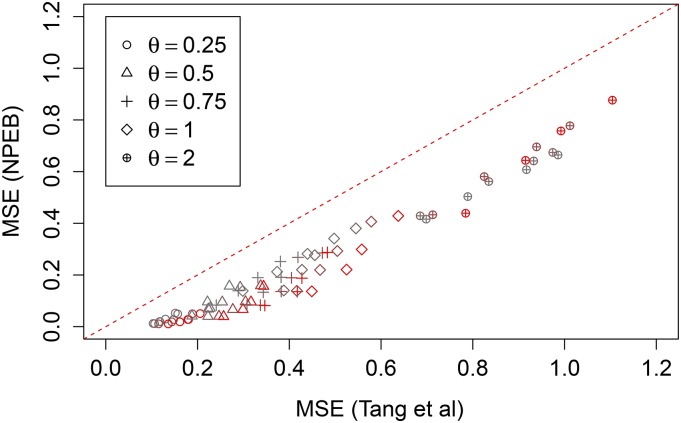
Figure 4 is a scatterplot of the MSE of estimates using the method of Tang et al. (2002) compared to those obtained using NPEB for simulations over the parameters in the multidimensional grid described in Table 1. We see that Robbins’ (1955) method always performs better than Tang et al.’s (2002) approach as measured by MSE.

Figure 4.

Accuracy of NPEB method vs. Tang et al.’s (2002) method. The NPEB method performs better than Tang et al.’s method in terms of MSE across the range of parameters in the multidimensional grid described in Table 1. Different values of θ are plotted using different shapes, and different values of m are plotted using different colors (large values are in red). In the dashed line we plot $y=x.$

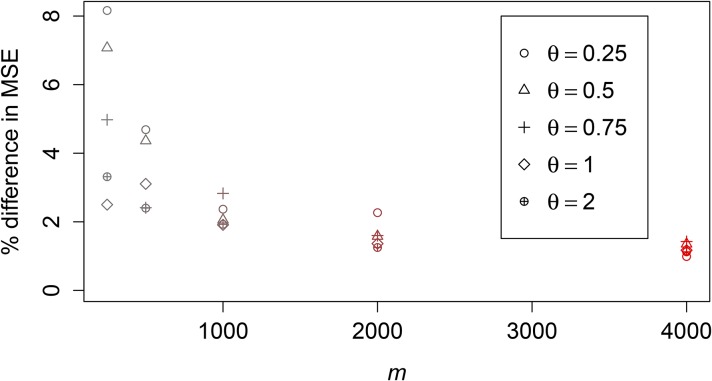
As we increase m, our estimates become more and more accurate: The NPEB MSE converges to the Bayes MSE where the true prior is assumed (Robbins 1955). We illustrate this for $g=0,$ $d=0,$ $n=2,$ and $0.25<\mathit{\theta }<2.0$ in Figure 5. The parametric Bayes estimates were obtained by assuming (correctly) that the values $T_i$ were drawn from an exponential distribution with parameter θ. We update the prior on $T_i$ with the observed number of mutations $x_i$ and in this way obtain the posterior on $T_i.$ We then report the mean of this posterior (see Equation 2). For m = 250, the MSE of the NPEB estimator is, depending on θ, ∼3.5–7.4% higher than the MSE of the Bayesian estimator using the correct prior. For $m\mathrm{=}4000,$ the difference is even smaller, with an increase of only ∼1.2%.

Figure 5.

NPEB vs. Bayes with true prior assumed. We plot $\left(\mathrm{MS}{\mathrm{E}}_{\mathrm{NPEB}}-\mathrm{MS}{\mathrm{E}}_{\mathrm{Bayes}}\right)/\mathrm{MS}{\mathrm{E}}_{\mathrm{Bayes}}$ for different values of m, which we vary in color, and different values of θ, which we vary in shape. For the parametric Bayes case, we assume as a true prior a constant population size and a divergence time of 0. We use a sample size of 2.

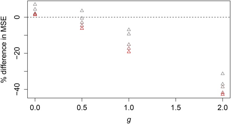
We found that when the assumed prior is not true, the Robbins estimator performs better than the parametric Bayesian estimator as long as m is big enough and the assumed prior is different enough from the true prior (Robbins 1955). We illustrate this in a particular case, for different values of $g>0,$ when the prior assumes $g=0,$ and for demographic parameter values $d=0$ and $\theta =0.5$ in Figure 6. It is worth noting that as we increase m, we also increase the number of loci $m*$ for which we are estimating the TMRCA. For this reason, the raw MSEs (e.g., Figure 4) are not completely comparable across different values of m, as they depend on this value $m*$ (see Equation 7).

Figure 6.

NPEB vs. Bayes with wrong prior assumed. Here we assume as a prior a constant population size, but in reality the exponential growth rate varies between 0 and 2 (see x-axis). The value of θ is 0.5, and the sample size is 2. Values of m range from 250 (in gray) to 4000 (in red).

In summary, our method performs better than Tang’s method across the entire range of tested parameters. Unsurprisingly, the parametric Bayesian estimator performs better than the empirical Bayes estimator when the true prior is assumed. However, our method can outperform the parametric Bayesian estimate in terms of MSE when the assumed prior is incorrect.

Admixture case study

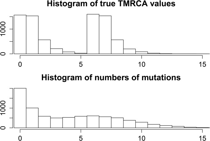
We also consider the special case of admixture, as a more complicated demographic history. In this case, we can still assume that the true TMRCAs are independent and identically distributed, but this time according to a more complicated distribution that exhibits bimodality (see Figure 7). Using again the program MSMS (Ewing and Hermisson 2010), we simulate the genealogies of pairs of just admixed individuals. Their parent populations diverged 6 time units in the past, with 50% of the genetic material in the sample originating from the first population and 50% from the second population. This means that 50% of sampled lineages will not be able to coalesce before 6 time units in the past. We fix $\mathit{\theta }\mathrm{=}1$ and consider $\mathit{m}\mathrm{=}8000$ independently segregating loci. Histograms of the true MRCAs and the number of mutations per site are shown in Figure 7, the latter being equal to Tang’s estimator in this case ($\mathit{\theta }=1$). We can see that there is considerable bimodality in the TMRCAs, which translates to bimodality in the number of mutations at different loci.

Figure 7.

Histograms of true and inferred TMRCAs in the admixture model. We can see that the number of mutations follows a similar distribution to the true times, but with higher variance. Tang et al.’s (2002) estimate of the TMRCA is proportional to the number of mutations.

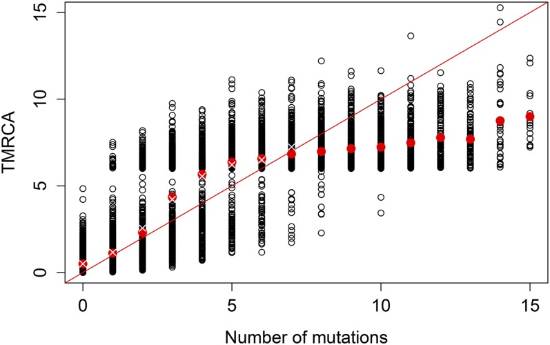
Plotting the true TMRCAs vs. the inferred TMRCAs using the two methods reveals that the true TMRCAs are appropriately shrunk using our method and that Tang’s method especially overestimates the TMRCAs in cases where there are a lot of mutations and underestimates them in cases where there are very few mutations (see Figure 8). We used 0.2 as a cutoff value, such that any points with variance >0.2 are not displayed. Note that Figure 8 represents a single (although typical) run of the algorithm. How well the NPEB ends up approximating the true TMRCA depends somewhat on the stochasticity of the data.

Figure 8.

Comparison of different methods in admixture model. In black circles is a scatterplot of the number of mutations at a locus and the true TMRCA at that locus. The red dots represent the average TMRCA for each locus with a given number of mutations. Values on the red diagonal line for each number of mutations represent estimates of the TMRCA using Tang et al.’s (2002) method, which tends to overestimate the value of the TMRCA when there are a large number of mutations and underestimate it when there are a small number of mutations. The white crosses represents NPEB estimates of the TMRCA for loci with zero to seven mutations. We do not report NPEB estimates of the TMRCA above seven mutations because the variance of the estimate is greater than our cutoff value, 0.2.

Analysis of TMRCAs from human genomes

We also apply our method to data from 37,574 neutrally evolving autosomal loci from a European and a Bantu individual (Gronau et al. 2011). Each interlocus distance is at minimum 50,000 bp, a distance deemed sufficiently high by Gronau et al. (2011) that the genealogies can be assumed to be approximately uncorrelated. These presumably neutral loci are 1000 bp in length and were chosen to avoid recombination hotspots. We remove any masked bases and reduce all of our loci to 900 bp, by truncating loci with >900 unmasked bases and removing loci with <900 unmasked bp. We use Gronau et al.’s (2011) estimate of the mutation rate of $0.7\times {10}^{-9}$ mutations per site per year and for the sake of illustration assume no variation in mutation rate across these loci, which we would otherwise control for by varying the length of each locus. Because of diploidy, we have a sample of size 2 for each individual.

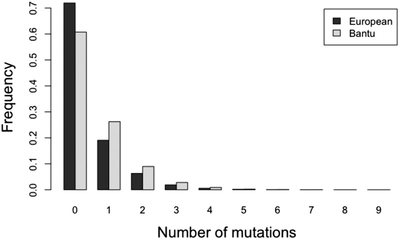
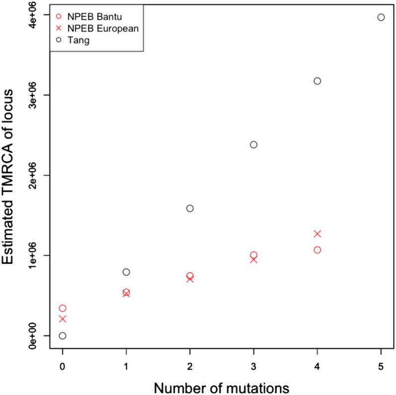
The distribution of numbers of mutations (or heterozygous sites) is different in the case of the Bantu and the European (see Figure 9), which we might attribute to the well-known bottleneck in the ancestry of European populations (Voight et al. 2005; Keinan et al. 2007). In particular, the average number of pairwise differences is greater for the Bantu than for the European. In Figure 10, we plot the inferred TMRCA at each locus for each of these two genomes. We note that, unlike with our method, the TMRCAs estimated using Tang’s method do not vary depending on the population. Using our method to estimate TMRCAs, we find that the calibration is less intense for the European sample than it is for the Bantu sample, which makes sense in light of the fact that the frequency of sites with exactly $x_i$ mutations decreases more sharply as $x_i$ increases for the European sample (Figure 9).

Figure 9.

Frequency histogram of the number of heterozygote sites in a Bantu and a European individual.

Figure 10.

Estimated TMRCA at loci with different numbers of mutations. We compare the NPEB method and Tang et al.’s (2002) method in estimating the TMRCA of different loci in a Bantu individual and a European individual. Tang et al.’s method does not depend on the distribution of the number of mutations in the population. We do not report NPEB estimates of the TMRCA above four mutations because their approximated variance is greater than our cutoff value.

Discussion

We have shown that the problem of estimating the TMRCA of a sample can be framed in such a way that it allows for the use of NPEB methods, such as a modified Robbins’ (1955) method. The advantage of these methods is that they use data from all loci to efficiently account for the randomness of mutation, through which loci with the same TMRCA can have very different numbers of segregating sites. In all of our simulations, Robbins’ (1955) method, one of the simplest NPEB methods, showed radical improvement over Tang et al.’s (2002) maximum-likelihood method (this is because the method makes use of a lot more of the available information). It also performed very well against a parametric Bayesian method in which it is assumed that the true prior for TMRCA is known.

It is particularly useful in that Robbins’ (1955) method provides reliable estimates of the TMRCA even when the mutation rate is very low. Many of the nucleotide sequences we simulated had 0 segregating sites. Our method was nonetheless reliably able to infer TMRCA at these loci, as long as there was enough information from other independently segregating loci. The other benefit of our method is that it does not require any prior assumptions on demographic history. We ran simulations using simple models of population expansion and divergence and showed that our method is effective in a wide variety of demographic scenarios.

For all cases where the genealogies uniting the sampled sequences are known, as for example when the sample is of size 2, the NPEB estimate may be calculated simply and directly using Equation 3. However, this method is somewhat limited to loci with sufficiently common numbers of segregating sites. It does not perform well with outliers, i.e., when $m_{x_i}$ is small.

More effective yet complicated NPEB approaches involve estimating the distribution $\widehat{G}$ of the $T_i$ from the data. Laird (1978) proved that the distribution of $T_i$ that maximizes the likelihood of the data is a discrete distribution over finitely many points j. An estimate of this distribution can be obtained using the expectation-maximization algorithm (Dempster et al. 1977). We can then get estimates of each individual $T_i$ by using Bayes rule with $\widehat{G}$ as a prior:

$$E\left[T_i|X_i=x_i\right]=\frac{{\displaystyle {\sum }_{k=1}^j{T}_{\left(k\right)}P\left(x_i|T_{\left(k\right)}\right)\widehat{G}\left(T_{\left(k\right)}\right)}}{{\displaystyle {\sum }_{k=1}^{j}P\left(x_i|T_{\left(k\right)}\right)\widehat{G}\left(T_{\left(k\right)}\right)}}$$ (8)

This approach is superior to Robbins’ (1955) method in that conditions of monotonicity and convexity are satisfied, and its success does not depend on the use of a squared error loss function over a general loss function (Carlin and Louis 2000). However, it involves much more computation than Robbins’ method. In this article, we concentrated on Robbins’ method as our goal was to show that there is information at independent loci and that even the simplest NPEB method performs quite well, especially compared to the maximum-likelihood approach.

Literature Cited

- Brookfield J., 1997. Importance of ancestral DNA ages. Nature 388: 134. [DOI] [PubMed] [Google Scholar]
- Carlin B., Louis T., 2000. Bayes and Empirical Bayes Methods for Data Analysis. Chapman & Hall CRC, Boca Raton, FL. [Google Scholar]
- Dempster A., Laird N., Rubin D., 1977. Maximum likelihood from incomplete data via the EM algorithm. J. R. Stat. Soc. B 39: 1–38. [Google Scholar]
- Donnelly P., Tavaré S., Balding S., Griffiths D., 1996. Estimating the age of the common ancestor of men from the zfy intron. Science 272: 1357–1359. [DOI] [PubMed] [Google Scholar]
- Dorit R., Akashi H., Gilbert W., 1995. Absence of polymorphism at the zfy locus on the human Y chromosome. Science 268: 1183–1185. [DOI] [PubMed] [Google Scholar]
- Ewing G., Hermisson J., 2010. MSMS: a coalescent simulation program including recombination, demographic structure and selection at a single locus. Bioinformatics 26: 2064–2065. [DOI] [PMC free article] [PubMed] [Google Scholar]
- Felsenstein J., 2006. Accuracy of coalescent likelihood estimates: Do we need more sites, more sequences, or more loci? Mol. Biol. Evol. 23: 691–700. [DOI] [PubMed] [Google Scholar]
- Fu Y., Li W., 1996. Estimating the age of the common ancestor of men from the zfy intron. Science 272: 1356–1357. [DOI] [PubMed] [Google Scholar]
- Gale W., Church K., 1990. Estimation procedures for language context: poor estimates are worse than none. COMPSTAT Proc. Comput. Stat. 9: 69–74. [Google Scholar]
- Gale W. A., Church K. W., 1994. What’s wrong with adding one?, pp. 189–200 in Corpus-Based Research into Language, edited by N. Oostdijk and P. de Haan. Rodopi, Amsterdam. [Google Scholar]
- Good I., 1953. The population frequencies of species and the estimation of population parameters. Biometrika 40: 237–264. [Google Scholar]
- Griswold C., Baker A., 2002. Time to the most recent common ancestor and divergence times of populations of common chaffinches (Fringilla coelebs) in Europe and North Africa: insights into Pleistocene refugia and current levels of migration. Evolution 56: 143–153. [DOI] [PubMed] [Google Scholar]
- Gronau I., Hubisz M., Gulko B., Danko C., Siepel A., 2011. Bayesian inference of ancient human demography from individual genome sequences. Nat. Genet. 43: 1031–1034. [DOI] [PMC free article] [PubMed] [Google Scholar]
- Hailer F., V., Kutschera B., Hallstrom D., Klassert S. Fain et al, 2012. Nuclear genomic sequences reveal that polar bears are an old and distinct bear lineage. Science 336: 344–347. [DOI] [PubMed] [Google Scholar]
- Hammer M., 1995. A recent ancestry for the human Y chromosomes. Science 378: 376–378. [DOI] [PubMed] [Google Scholar]
- Hobolth A., Christensen O., Mailund T., Schierup M., 2007. Genomic relationships and speciation times of human, chimpanzee, and gorilla inferred from a coalescent hidden Markov model. PLoS Genet. 3: 294–305. [DOI] [PMC free article] [PubMed] [Google Scholar]
- Jakubiczka S., Arnemann J., Cooke H., Krawczak M., Schmidtke J., 1989. A search for restriction fragment length polymorphism on the human Y chromosome. Hum. Genet. 84: 86–88. [DOI] [PubMed] [Google Scholar]
- Keinan A., Mullikin J. C., Patterson N., Reich D., 2007. Measurement of the human allele frequency spectrum demonstrates greater genetic drift in East Asians than in Europeans. Nat. Genet. 39: 1251–1255. [DOI] [PMC free article] [PubMed] [Google Scholar]
- Laird N., 1978. Nonparametric maximum likelihood estimation of a mixing distribution. J. Am. Stat. Assoc. 73: 805–811. [Google Scholar]
- Li H., Durbin R., 2011. Inference of human population history from individual whole-genome sequences. Nature 475: 493–496. [DOI] [PMC free article] [PubMed] [Google Scholar]
- Lidstone G., 1920. Note on the general case of the Bayes-Laplace formula for inductive or a posteriori probabilities. Trans. Faculty Actuaries 8: 182–192. [Google Scholar]
- R Core Team , 2015. R: A Language and Environment for Statistical Computing. R Foundation for Statistical Computing, Vienna. [Google Scholar]
- Rice J., 2007. Mathematical Statistics and Data Analysis, Ed. 3 Duxbury Press. Belmont, CA. [Google Scholar]
- Robbins H., 1955. An empirical Bayes approach to statistics. Proceedings of the Third Berkeley Symposium on Mathematical Statistics and Probability, Vol. 1, pp. 157–164. University of California Press, Berkeley. [Google Scholar]
- Rosenberg N., Feldman M., 2002. The relationship between coalescence times and population divergence times, pp. 130–164 in Modern Developments in Theoretical Population Genetics, edited by Slatkin M., Veuille M. Oxford University Press, New York. [Google Scholar]
- Saunders I. W., Tavaré S., Watterson G. A., 1984. On the genealogy of nested subsamples from a haploid population. Adv. Appl. Probab. 16: 471–491. [Google Scholar]
- Tajima F., 1983. Evolutionary relationship of DNA sequences in finite populations. Genetics 105: 437–460. [DOI] [PMC free article] [PubMed] [Google Scholar]
- Tang H., Siegmund D., Shen P., Oefner P., Feldman M., 2002. Frequentist estimation of coalescence times from nucleotide sequence data using a tree-based partition. Genetics 105: 437–460. [DOI] [PMC free article] [PubMed] [Google Scholar]
- Turner, R., 2015 Iso: Functions to Perform Isotonic Regression R package version 0.0-17. Available at: http://CRAN.R-project.org/package=Iso.
- Vigilant L., Stoneking M., Harpending H., Hawkes K., Wilson A., 1991. African populations and the evolution of human mitochondrial DNA. Science 253: 1503–1507. [DOI] [PubMed] [Google Scholar]
- Voight B. F., Adams A. M., Frisse L. A., Qian Y., Hudson R. R., et al. , 2005. Interrogating multiple aspects of variation in a full resequencing data set to infer human population size changes. Proc. Natl. Acad. Sci. USA 102: 18508–18513. [DOI] [PMC free article] [PubMed] [Google Scholar]
- Walsh B., 2001. Estimating the time to the most recent common ancestor for the Y chromosome or mitochondrial DNA for a pair of individuals. Genetics 158: 897–912. [DOI] [PMC free article] [PubMed] [Google Scholar]
- Watterson G., 1975. On the number of segregating sites in genetical models without recombination. Theor. Popul. Biol. 7: 256–276. [DOI] [PubMed] [Google Scholar]
- Weiss G., von Haeseler A., 1996. Estimating the age of the common ancestor of men from the zfy intron. Science 272: 1359–1360. [DOI] [PubMed] [Google Scholar]
- Whitfield L., Sulston J., Goodfellow P., 1995. Sequence variation of the human Y chromosome. Nature 378: 379–380. [DOI] [PubMed] [Google Scholar]
Associated Data
This section collects any data citations, data availability statements, or supplementary materials included in this article.
Data Availability Statement