Mapping cell populations in flow cytometry data for cross‐sample comparison using the Friedman–Rafsky test statistic as a distance measure

Abstract

Flow cytometry (FCM) is a fluorescence‐based single‐cell experimental technology that is routinely applied in biomedical research for identifying cellular biomarkers of normal physiological responses and abnormal disease states. While many computational methods have been developed that focus on identifying cell populations in individual FCM samples, very few have addressed how the identified cell populations can be matched across samples for comparative analysis. This article presents FlowMap‐FR, a novel method for cell population mapping across FCM samples. FlowMap‐FR is based on the Friedman–Rafsky nonparametric test statistic (FR statistic), which quantifies the equivalence of multivariate distributions. As applied to FCM data by FlowMap‐FR, the FR statistic objectively quantifies the similarity between cell populations based on the shapes, sizes, and positions of fluorescence data distributions in the multidimensional feature space. To test and evaluate the performance of FlowMap‐FR, we simulated the kinds of biological and technical sample variations that are commonly observed in FCM data. The results show that FlowMap‐FR is able to effectively identify equivalent cell populations between samples under scenarios of proportion differences and modest position shifts. As a statistical test, FlowMap‐FR can be used to determine whether the expression of a cellular marker is statistically different between two cell populations, suggesting candidates for new cellular phenotypes by providing an objective statistical measure. In addition, FlowMap‐FR can indicate situations in which inappropriate splitting or merging of cell populations has occurred during gating procedures. We compared the FR statistic with the symmetric version of Kullback–Leibler divergence measure used in a previous population matching method with both simulated and real data. The FR statistic outperforms the symmetric version of KL‐distance in distinguishing equivalent from nonequivalent cell populations. FlowMap‐FR was also employed as a distance metric to match cell populations delineated by manual gating across 30 FCM samples from a benchmark FlowCAP data set. An F‐measure of 0.88 was obtained, indicating high precision and recall of the FR‐based population matching results. FlowMap‐FR has been implemented as a standalone R/Bioconductor package so that it can be easily incorporated into current FCM data analytical workflows. © 2015 International Society for Advancement of Cytometry

As the most mature single‐cell analysis technology, flow cytometry (FCM) has been widely applied in the diagnosis and characterization of cancers, infectious diseases, neurological disorders, immune system diseases, and hematological disorders 1. In a typical FCM study, tens to thousands of blood or tissue samples are processed to quantify cellular characteristics (e.g., protein expression levels) in individual cells. A modern polychromatic flow cytometer can measure up to 27 cellular characteristics for millions of cells in each sample 2. To characterize and differentiate FCM samples from different experimental conditions/perturbations, cell populations need to be identified and their variations across samples need to be quantified and assessed. For example, regulatory T cells are known to suppress a variety of pathological and physiological immune responses. In peripheral blood of individuals with autoimmune disease, regulatory T cells tend to exist in smaller proportions than in healthy controls 3. Cell populations may also differ because of an individual's inherited biological traits. For example, immunoglobulin E (IgE) is an antibody that is elevated when the immune system overreacts to environmental allergens, such as pollen. In individuals that are predisposed to allergic responses, elevated numbers of circulating B cells expressing the high‐affinity IgE receptor (CD23) can be found 4.

Historically, manual gating has been used as the methodology of choice to delineate cell populations sharing common characteristics in FCM data. This graphically driven approach relies on the sequential application of manually drawn boundaries (i.e., gates) to distinguish cells on uni‐ or bi‐axial data plots. The placement of manual gating boundaries is subjective and depends on the experience of the data analyst. In recent years, computational gating methods have made significant advances in identifying cell populations at the individual sample level 5. Model‐based computational gating approaches, such as Gaussian and multivariate skew‐t mixture model fitting 6, 7, 8, 9, employ statistical assumptions on the shape and location of cell population distributions. Non‐model‐based methods, such as grid‐based density clustering 10 and spectral clustering 11 algorithms, group cells into homogeneous populations based on unsupervised data clustering.

After cell populations are identified in individual samples, the next step is to map cell populations between samples so that cell population characteristics, such as marker expression levels and proportions, can be compared across the sample set. In manual gating approaches, the gating boundaries drawn on one sample are often directly applied to another sample. However, marker expression levels of equivalent cell populations can shift between different samples due to technical artifacts and natural biological variability. Technical artifacts can be unintentionally introduced during data acquisition, especially in multicenter clinical studies where samples are prepared at several sites, with slight differences in sample preparation procedures, staining protocols, and instrument settings. Biological variability in marker expression can occur due to the complex interplay of genome sequence polymorphisms, especially in outbred human populations. Indeed, the effects of technical artifacts and biological variation can be difficult to distinguish. These inherent sources of variability in marker expression make the cell population mapping step using direct application of manual gating boundaries problematic for cross‐sample comparisons.

To our knowledge, there is no standalone method implementation focused solely on cell population matching. Probability binning 12 is able to compare multivariate distributions between FCM samples but it remains unclear how it can be adapted to compare population‐level data as cell populations frequently shift expression distributions across samples. Finak et al. 13 compared sample‐level variability in cell population marker expression among fluorescent channel transformation methods (e.g., bi‐exponential or generalized Box‐Cox). Variation between cell population locations is defined as the sum of squared deviations of the cell population locations from the mean cell population location across FCM samples. Small intersample variations in cell population locations are associated with low population misclassification rates. Other existing approaches, including FLAME 7, HDPGMM 6, JCM 9, and flowMatch 14, bundle the cell population identification method and cross‐sample mapping function together, with the mapping component operating under the principle of global template finding. In FLAME 7, mapping cell populations across samples is the last step of their computational gating method. Each sample is modeled as a mixture of cell populations, each with a multivariate skew‐t distribution. The modes of cell population distributions are pooled together across samples to establish a global template of cell populations, marked by their mode locations. The sample cell populations are then matched to the global populations based on the respective mode locations. In both HDPGMM 6 and JCM 9, a multilevel modeling approach is applied to simultaneously identify cell populations and map populations across samples. A global template is generated based on shared location and shape characteristics among cell populations across samples in the same cohort. JCM ascribes multivariate skew‐t distributions to the cell populations as in FLAME, while the HDPGMM assumes Gaussian distributions for the cell populations. Both methods perform the mapping step automatically while the population is being identified, which precludes their implementation with other data clustering methods. When a new sample is added to the data set, HDPGMM needs to be rerun on all samples to generate a new hierarchy that could be different from the original one even for the same sample. JCM directly compares the new sample with the population location and shape parameters at the cohort level using the Kullback–Leibler divergence measure (KL distance). In flowMatch 14, samples are organized into a hierarchy based on overall shape similarity between sample cell populations. The KL distance is also used to quantify the multivariate similarity between cell populations. Two samples are merged together under the hierarchy when the total between‐sample KL distance is minimized. The root of the hierarchy is the global template of cell populations. These existing methods all require the composition of a global template, which can be error‐prone without careful selections of mapping thresholds at each comparison. The construction of the template is also very sensitive to the clustering or gating procedures. Some of these methods do not calculate the degree of similarity between cell populations, limiting the ability to map heterogeneous cell populations across samples.

Here we describe a novel method, FlowMap‐FR, that uses a data‐driven approach for cell population mapping. FlowMap‐FR directly compares the cell populations between samples using the Friedman–Rafsky (FR) test statistic (FR statistic, 15)—a nonparametric multivariate statistical measure utilizing a minimum spanning tree approach to describe the “ordering” of values in multidimensional space. The FR statistic has been used as a similarity measure in statistical pattern recognition 16, image retrieval 17, and image registration 18. The basic principle is to “sort” the events from any two merged cell populations (e.g., cell populations in different samples being tested to determine if they are equivalent) based on edge connections in a minimum spanning tree constructed from the marker expression levels of each cell. The cell populations being compared are considered to be equivalent if their respective member events are randomly dispersed in the tree, and are different if the events of the same membership tend to congregate in different branches of the tree. Thus, FlowMap‐FR evaluates cell population similarity by computing a statistical distance measure for every possible population pair in a cross‐sample mapping problem. FlowMap‐FR is a standalone method that can be applied to mapping cell populations delineated by manual gating or computational clustering procedures. We evaluated the performance of FlowMap‐FR in simulation experiments designed to mimic commonly observed scenarios of sample variability for mapping cell populations in which differences in cell population proportions occur between samples, slight differences in marker expression levels in equivalent populations occur between samples, and a cell population in one sample is inappropriately divided into two by overpartitioning in comparison with another sample. We also compared the performance of FlowMap‐FR with the symmetric version of KL distance used in flowMatch 14 using both simulated and real data, and applied it to match gated populations from a FlowCAP benchmark data set 5.

Methods

Terminology

In a given FCM experiment, the levels of a number of different quantitative markers (features) are measured in individual cells. Each cell can then be represented as a feature vector of marker levels in d‐dimensional space. A cell population is defined as a homogenous group of cells sharing similar quantitative levels for all markers measured, and can be delineated by manual or computational gating methods as a feature vector cluster in multidimensional space. The number of features evaluated in the FCM experiment is equivalent to the number of dimensions of the multivariate vector. When comparing two cell populations, the events from the different populations can be combined to form pooled data. A graph can be constructed on the pooled data, where the nodes represent the cell events and the edges represent the Euclidean distance between the multivariate feature vectors.

Overview of FlowMap‐FR

Figure 1 shows the hypothetical FCM assay of 4 expression markers (CD4, CD45RA, SLP76, ZAP70) for two different biological samples. The goal of cross‐sample comparison is to determine if either Cell Population (CP)red or CPgreen in sample B is equivalent to the CPblue reference cell population in sample A. The bi‐axial plots indicate similarity between CPblue and CPgreen in all expression marker levels except for CD4, while CPblue and CPred are similar in all markers and would therefore be considered to be equivalent. The goal of any quantitative method for cross‐sample comparison would be to accomplish cell population mapping by objectively making this distinction using cell populations delineated by any data transformation procedure or gating method, including manual gating or algorithmic clustering.

Figure 1.

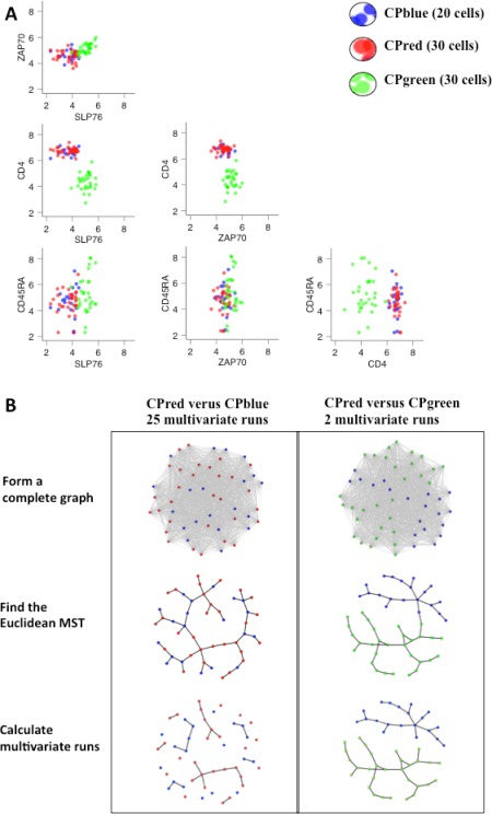
Multivariate run calculation. This figure illustrates the general problem of mapping cell populations between samples using FCM data with four marker channels (CD4, CD45RA, ZAP70, and SLP76). In this example, we want to determine if Cell Population (CP)red in or CPgreen in Sample B corresponds to CPblue in Sample A. (A) Marker level distributions of CPblue in comparison with CPred and CPgreen. Note that the marker level distributions for CPblue and CPgreen are similar for ZAP70 and SLP76, but differ for CD4. Based on this difference, we would infer that CPgreen in Sample B is different from CPblue in Sample A. On the other hand, the marker expression distributions for CPblue and CPred are similar for all four markers. Based on these similarities, we would infer that CPred in Sample B is equivalent to CPblue in Sample A. (B) Multivariate run calculation for the CPblue/CPred and CPblue/CPgreen comparisons. The FlowMap‐FR application of the Friedman–Rafsky test proceeds through the following steps separately for CPblue/CPred and CPblue/CPgreen comparisons: merge the cell event data from the reference (CPblue) and test (CPred or CPgreen) populations, calculate the pairwise Euclidean distances between all events (nodes) to form a complete Euclidean graph, find the minimum spanning tree that connects all nodes in the Euclidean graph, remove the edges that connect nodes derived from different cell populations, and determine the number of subgraphs remaining (which equals the number of edges connecting nodes between the two different cell populations plus 1). In the case of the CPblue versus CPgreen comparison, the number of runs would equal 2. For the CPblue versus CPgreen comparison, the number of runs would equal 25. Relatively small run values indicate that the cell populations being compared are distinct because their events are segregated in multivariate space. [Color figure can be viewed in the online issue, which is available at wileyonlinelibrary.com.]

The FlowMap‐FR method for cross‐sample mapping described here utilizes the Friedman–Rafsky multivariate generalization of the Wald–Wolfowitz run statistic for comparing two data distributions to determine if they have been sampled from the same global data population. Wald and Wolfowitz 19 described a statistical procedure to compare univariate nonparametric distributions by merging the values from two different data sets into an ordered list and quantifying the number of runs that connect values derived from the same data set. The number of runs is thus associated with the tendency of the values to cluster together according to their respective membership in the data sets. A small number of runs connecting values from the same data set suggest that the values have been sampled from more than one distribution. Friedman and Rafsky 15 proposed a generalization of this approach for multivariate data, in which value order is determined based on proximity in a minimum spanning tree constructed in multivariate space.

The basic idea is to connect the events across the two cell populations to be compared according to their similarity in expression of all d markers using a minimum spanning tree. The individual cell events are represented as nodes on the tree. The distance between two nodes is calculated as the Euclidean distance in d‐dimensional space. The FR statistic quantifies the multivariate similarity of nodes from any two underlying distributions in the minimum spanning tree (MST). The FR statistic also controls for the size of the MST across comparisons and the topological structure of the MST. We calculate the FR statistic comparing each pair of cell populations. For example, a comparison of two biological samples with n ₁ and n ₂ cell populations would involve n ₁ × n ₂ total comparisons.

FlowMap‐FR estimates the FR statistic based on controlled statistical sampling of the events in data pooled from the two cell populations being compared. Each controlled statistical sample taken from this pool comprised events sampled to be proportional to those in the original cell population pair (above some minimum number of events). This controlled statistical sampling approach is employed because the computing time for calculating a minimum spanning tree is dependent on the number of nodes, that is, total number of events involved in a cell population comparison pair.

Finding the Minimum Spanning Tree

We begin by mixing events from two cell populations under comparison while keeping track of their population membership. The mixture of events is henceforth referred to as the pooled data. We then take S controlled statistical samples of N events randomly selected from the pooled data, without replacement. Each controlled sample maintains a constant ratio of events from the two cell populations, calculated from the pooled data before any event selection. For every controlled statistical sample, we compute the Euclidean distance between every pair of events based on the expression level of all markers. A complete weighted undirected graph is constructed based on the N‐by‐N distance matrix. We then use Prim's algorithm 20, 21, 22 to find the minimum spanning tree (MST) on the graph (see Supporting Information Methods for more details). The distance between events on the minimum spanning tree corresponds to the dissimilarity of their marker expressions in d‐dimensional space. Therefore, events with similar marker expression levels are placed near each other on the MST branches. Figure 1 depicts the schematic illustration of the MST construction steps.

Friedman–Rafsky Statistic Computation

Central to the Friedman–Rafsky (FR) statistic are the multivariate “runs” in the Euclidean MST. The multivariate runs are the set of subtrees in the MST consisting of connected events from a single cell population (see Supporting Information Methods for more background of the FR statistic). For each controlled sample MST based on N events, we remove the edges connecting events derived from different cell populations. Because any removal of an edge in an MST breaks the tree into two disjoint subtrees, the number of subtrees in an MST is equal to the number of removed edges (G) plus 1. Thus, the number of multivariate “runs” R is equal to G + 1.

The FR statistic compares the observed with the expected number of multivariate runs in a given MST from two equivalent population distributions, and then standardizes the difference by the variance of the multivariate runs. Given two cell populations X and Y of event sizes m and n, respectively, with N total events, the expected number of multivariate runs E[R] is equal to one plus the expected number of edges. For the N − 1 edges of the given MST, the probability that an arbitrarily selected edge connecting X and Y (or Y and X) is the proportion of events in N belonging to X, m/N (or n/N if considering edges connecting Y and X) multiplied by the probability that the edge connects to a node in Y, n/(N − 1) (or m/(N − 1) if considering Y–X edges). Hence, the expected number of edges is

$$\mu = E\left(R\right) = \frac{2mn}{N}+1$$

The variance of the number of runs in a given MST is dependent on the corresponding topological feature—the total number of edge pairs sharing common nodes (C), which is $\left(\genfrac{}{}{0pt}{}{\mathrm{N}-1}{2}\right)$ in a graph of N nodes. Hence, the variance reflects the range of runs possible given the composition of membership events in a cell population pair comparison, and

$${\sigma }^2 = \frac{2mn}{N-1}\left\{\frac{2mn-N}{N}+\frac{\left(C-N+2\right)\left(m+N\left(N-1\right)-4mn+2\right)}{\left(N-2\right)\left(N-3\right)}\right\}$$

Details of the derivation can be found in Friedman and Rafsky 15. The FR statistic (w) is then defined as

$$w = \frac{\mathrm{R}-\mu }{\sigma }$$

The median FR statistic from the S controlled statistical samples of the pooled data is taken as the estimated measure for similarity between the two cell populations. The estimated FR statistic is multiplied by −1 to compute an FR‐based distance measure, where a small value indicates high degree of similarity and a large value indicates high degree of dissimilarity. This FR‐based distance measure can then be used with various clustering methods to group cell populations across samples (e.g., by hierarchical clustering).

Hypothesis Testing Using the FR Statistic

We can also use the estimated FR statistic to perform a statistical test where the null hypothesis is that the two cell populations follow the same distribution. The P values of the FR statistical test are computed under the assumption that the standardized FR statistic follows a normal distribution 15. A large P‐value is evidence that the cell populations in the comparison are probably similar in their distributions, while a small P‐value is evidence that the cell populations are probably different in their distributions. In addition to cell population similarity, the P‐value of the FR statistic also depends on the number of controlled statistical samples of the pooled data (S) and the size of each controlled sample (N). For the analyses in this study, we chose a value of 10⁻⁷ for the P‐value threshold of the FR statistic where the number of true‐positive matched cell population pairs is maximized and the number of false‐positive cell population pairs is minimized. The threshold was chosen based on sampling parameters N = 200 and S = 200. Details of choosing the sampling parameters are described in the following section.

Sampling Parameters

In order to both reduce runtime and provide for consistent statistics, data sampling is necessary before the FR statistic is applied. With the controlled sampling approach, the FR statistic value in a pairwise comparison between two cell populations depends on the number of controlled samples (S), and the number of events in the pooled controlled sample (N). We assessed the precision (reflecting the extent of reproducibility of the controlled sampling procedure) and accuracy (indicating the biasedness of the estimated statistic as a function of the sampling procedure) of the FR statistic under N = 100, 200, and 400 and S = 100, 200, and 400. While increasing S results in a larger range of the FR statistics, the ranks of the population pairs remain the same, and the FR statistic value increases as N increases. Nonetheless, when mapping cell populations across two samples, the ranks of the population comparisons remain the same across varying N and S (Supporting Information Figs. S8A,B). The time complexity of the controlled sampling approach is assessed under N = 50, 100, 200, 400, 600, 800, and 1000 and S = 100, 200, and 400. The time complexity increased quadratically in the number of the events, but did not change across the number of controlled samples (Supporting Information Fig. S7A). FlowMap‐FR computes an adjacency matrix of similarity between N events based on Euclidean distance between the d‐dimensional measurement vectors. Prim's algorithm is then employed to find the MST of each controlled sample. The computing time of MST finding is known to increase quadratically in N in the Prim's algorithm when the similarity between the events is represented in an adjacency matrix (Supporting Information Figs. S7A,B). In summary, N and S are chosen to preserve the ranks of the FR statistics with balanced precision and accuracy as well as minimized computing time of MST.

Data Preprocessing

FlowMap‐FR is designed as a stand‐alone algorithm that can be applied to mapping cell populations derived from any gating procedures or any normalization methods. The input data contains ASCII files with each cell population's labels and marker expression levels derived from manual gating or automated gating method. Before applying FlowMap‐FR, the user needs to choose a transformation method to transform the raw data into equivalent quantitative ranges based on their data formats and use cases. We employed FCSTrans 22 for all the analyses in this article.

Data Simulation

In order to assess the performance of FlowMap‐FR under a variety of different population mapping scenarios, a simulated data set was constructed to closely mimic real FCM data. Data from FCM experimental samples vary in distributional shape depending on the sample's biological characteristics. In order to conduct a fair performance evaluation of our cell population mapping method, we sought to mimic possible sources of experimental sample variability in cell population characteristics. We selected a real data set that includes cell populations possessing features inherent to FCM data: sparseness of some populations but not others, skewness in the distribution of some cell population markers, high correlation between expression levels for a subset of markers, and flat density distributions for some markers. The real data were derived from an FCM experiment in which human peripheral blood was assayed with a four marker panel: CD14, CD23, CD3, and CD19 23. The FLOCK clustering algorithm 10 was used to identify nine distinct cell populations (CP1–CP9) in an FCS data file from one sample totaling 20,000 events.

Multivariate skew‐t distributions were employed to extract location, variance, and skewness parameters of each cell population in the real data. The estimated parameters of the fitted skew‐t distribution were then used to simulate a new data set that mimics the marker distributions observed for each reference cell population. A list of parameter settings can be found in Supporting Information Table S1. Figure 2A and 2B shows the cell population distributions for selected markers in the real sample and in the simulated sample, respectively. Complete bi‐axial distribution plots of the cell populations are shown in Supporting Information Figure S1A,B. An important FCM data feature is that some cell populations may overlap in some marker channels while being well separated in other dimensions. This can be illustrated by CP3 and CP9. Their marker expression levels are overlapping and correlated in the two‐dimensional scatter of CD23 and CD14 and also between CD3 and CD14. However, they are well separated based on CD19 marker expression levels.

Figure 2.

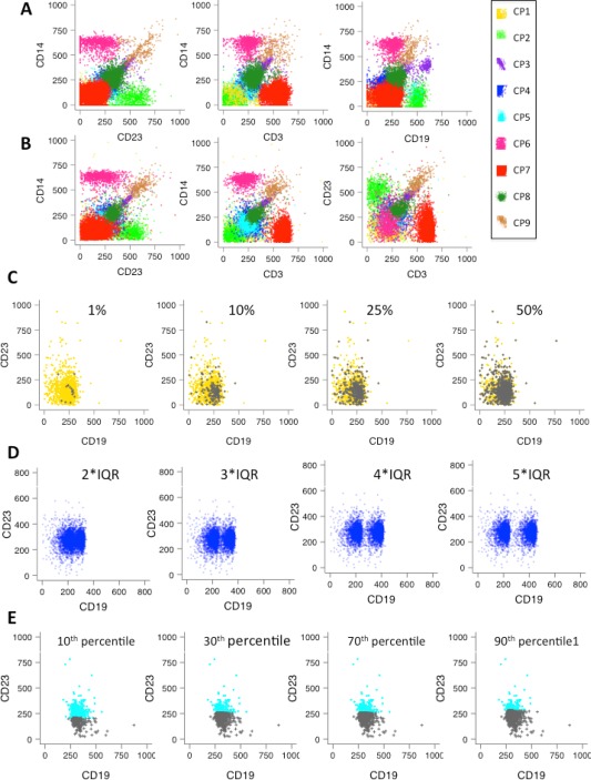
Data simulations and test scenarios. (A) Selected bi‐axial plots of the nine cell populations from an experimentally measured data set in four marker channels (CD14, CD23, CD3, and CD19). For each population, multivariate skew‐t distributions were fitted and the corresponding distribution parameters were determined. See Supporting Information Table 1 for the list of parameters. (B) Selected bi‐axial plots of the nine cell populations in the simulated data set. The skew‐t distribution parameters derived from fitting the original data were used to simulate the nine populations shown. The simulated cell populations mimic the original cell population in the correlation between markers and also the marker distributions. These parameters were employed to simulate cell populations throughout this study. The complete set of two‐dimensional plots is shown in Supporting Information Figure 1. (C) Scenario 1—Differences in cell populations between samples. Overlap between CP4 changed in proportion to 1%, 10%, 25%, and 50% (colored in green) and the original 2363 events in population CP4 in the reference population (colored in cyan). Scenario 2, in which the test cell population was deleted, is not shown but would essentially correspond to the first plot without the green events. (D) Scenario 3—Shifts in marker expression levels between samples. CP1 (colored in blue) shifted along CD19 to 2, 3, 4, and 5 units of interquartile range (IQR) of the CD19 distribution. (E) Scenario 4—A discrete cell population in one sample inappropriately divided into two by over‐partitioning in another sample. The original CP4 (colored in cyan) overlaid with the CP4 partitions below CD23 10, 30, 70, and 90^th percentile (colored in grey). [Color figure can be viewed in the online issue, which is available at wileyonlinelibrary.com.]

Evaluation Scenarios

In FCM data, cell populations may exhibit slight shifts in marker levels between biological samples or vary in the percent composition per sample between individuals or cohorts (i.e., varying proportions). The simulated data set was used to construct a series of test samples designed to mimic these real scenarios in cross‐sample comparison challenges to test the cell population mapping performance of FlowMap‐FR, as follows:

Scenario 1. Differences in cell population proportions between biological samples (Fig. 2C)

Test samples were constructed in which cell proportions were changed to 1%, 10%, 25%, 50%, 75%, 125%, and 150% of the original simulated cell population. Location and shape of the changed cell populations was maintained as in the original simulated cell populations. Each changed cell population was a statistical sample of events randomly generated with the same location and shape parameters as the original simulated cell population.

Scenario 2. Differences in cell population numbers between biological samples

Test samples were constructed in which one of the simulated cell populations from one biological sample was removed. The resulting test sample containing eight cell populations was compared with the original simulated sample containing nine cell populations.

Scenario 3. Shifts in marker expression levels between biological samples (Fig. 2D)

Test samples were constructed in which the simulated cell population from one biological sample is shifted along each marker channel one at a time. The unit of location shift is standardized for each cell population and defined as the interquartile range ( ${\text{IQR}}_{\mathrm{o},i})$ of the original simulated cell population along channel $i$, where ${\text{IQR}}_{\mathrm{o},i}$ = 75^th percentile − 25^th percentile of the original simulated cell population in channel $i$. For each of the nine cell populations, we simulated 1, 2, 3, 4, and 5 ${\text{IQR}}_{\mathrm{o},i}$ shifts along each marker channel. Denote ${\mu }_{\mathrm{o},i}$ as the original location of a cell population along channel $i$ and ${\mu }_{2,i}$ as the shifted location after 2 units of interquartile range shift. Then, ${\mu }_{2,i} = {\mu }_{\mathrm{o},i} + 2 \times {\text{IQR}}_{\mathrm{o},i}$.

Scenario 4. A discrete cell population in the reference sample inappropriately divided into two in the test sample by over‐partitioning (Fig. 2E)

Test samples were constructed in which the single simulated cell populations from the reference sample were divided into two partitions along the CD23 channel. Two sets of partition samples were simulated accordingly that include the upper and lower partitions above and below the 90^th, 80^th, 70^th, 60^th, 50^th, 40^th, 30^th, 20^th, and 10^th percentile of the corresponding CD23 levels.

Comparison with the Kullback–Leibler Divergence Measure

The results using the simulated scenarios was also evaluated using the symmetric version of Kullback–Leibler (referred to be SKL distance to distinguish from the original KL distance) divergence measure used in flowMatch to compare cell populations across multiple samples 14. The KL distance is known as an asymmetric distance measure between two distributions such that the values comparing CP1 to CP2 and CP2 to CP1 can differ. In flowMatch, a symmetric version of the KL distance (SKL) is employed under which the cell populations are assumed to follow multivariate normal distributions. Using this version, the KL distance is a function of means and variances of the cell populations. The SKL distance is achieved by averaging the two possible KL values in a single comparison. Given two cell populations i and j in d‐dimensional feature space, the KL value of comparing i against j is

$$\frac{1}{2}\left\{\text{log}\frac{\left|{\Sigma }_j\right|}{{|\Sigma }_i|}+tr\left({\Sigma }_j^{-1}{\Sigma }_i\right)+{\left({\mu }_j-{\mu }_i\right)}^T{\Sigma }_j^{-1}\left({\mu }_j-{\mu }_i\right)-d\right\}$$

where ${\mu }_{\mathrm{i}}$and ${\mu }_{\mathrm{j}}$ are d‐dimensional mean vectors of the expression markers of cell populations i and j, respectively, and ${\Sigma }_i$ and ${\Sigma }_j$are d‐dimensional variance–covariance matrices of the markers for cell populations i and j, respectively. We computed sample means and variances to approximate $\mu \mathrm{s}$ and ${\Sigma }^{}\mathrm{s}$to calculate the SKL distance values of the simulated cell populations as in the flowMatch implementation.

Mapping Cell Populations Across Multiple Real FCM Samples

FlowMap‐FR was applied to two real flow cytometry data sets to evaluate its performance in mapping cell populations across multiple real flow cytometry samples. The first evaluation investigated the ability of FlowMap‐FR to map cell populations that are known to be biological replicates across FCM samples. The second evaluation applied FlowMap‐FR to FCM samples collected from 30 different healthy individuals. In this data set, the individual cell populations within each sample and their equivalence between samples were delineated by expert manual gating as part of the FlowCAP challenges 5.

Real FCM data set #1

The first real data set evaluation included four FCM samples of peripheral blood mononuclear cells (PBMC) collected from two healthy individuals 24; the blood sample from each individual was divided into two biological replicates. Each sample was stained with four fluorophore‐labeled antibodies (marker panel: CD3, CD4, CD8, and CD19). Four cell populations were identified in each of the FCM samples using K‐means clustering (parameter setting: minimum 4 and maximum 20 clusters). The K‐means convergence criteria were set to minimize within‐cluster sum of squares while maximizing between‐cluster sum of squares. In order to perform cell population mapping across multiple samples, we computed the estimated FR statistics and FR‐based distance metric (FR multiplied by minus one) for all population pairs across the four FCM samples. The FR‐based distances were used as a similarity measure to group and map equivalent cell populations across samples. Hierarchical clustering with complete linkage was employed as the clustering method of choice. The cell populations were arranged in a hierarchy according to the FR distance to the other cell populations.

The FR‐based mapping approach was compared to flowMatch 14. flowMatch performs agglomerative clustering that repeatedly merges samples to form a template sample until there are no more samples to be added (meta‐clustering). First, a template sample is created from merging the two most similar samples, and the matched cell populations are combined to form a cell population. Then, a template sample is compared to all the other samples and merged with the sample that is most similar. This step continues until there are no more samples to be compared with. At each step, cell populations are mapped across samples when the two samples are merged into one template sample. A bipartite graph algorithm is employed to match two samples or to match a sample with a template sample when the sum of distances between cell populations is minimized. The performance of the FR statistic was compared with the SKL divergence metric within the flowMatch algorithm. Details of the bipartite algorithm underlying flowMatch are described in Supporting Information Methods.

Real FCM data set #2

This normal donor data set was one of the benchmark data sets included as part of the FlowCAP‐I challenge 5 and contained manually gated cell populations that can be used as a benchmark for evaluating the performance of FlowMap‐FR. A total of 30 FCM samples from normal healthy donors are included in the data set. Each sample was stained with a cocktail of 10 fluorochrome reagents, interrogating both cell surface and intracellular proteins. Expert manual gating by the data providers delineated 8 cell populations in each sample. To perform cell population mapping across multiple samples, we computed the estimated FR statistics for all population pairs across the 30 FCM samples (28,680 comparisons). Similar to real data set #1, hierarchical clustering with complete linkage was employed in order to organize the cell populations in a hierarchy according to FR distance. Based on the FR similarity hierarchy, cell populations were classified into eight sets of equivalent cell populations. The F‐measure approach was then used to evaluate the combined precision and recall performance of the new cell population labels in comparison with the cross‐sample equivalence determined by the original data providers.

Software Availability and Data Sharing

FlowMap‐FR is available in the R/Bioconductor flowMap package (http://bioconductor.org/packages/release/bioc/html/flowMap.html) and on Github (https://github.com/JoyceHsiao/flowMap). The simulated data file has been converted to FCS format and made publicly available through flowrepository.org under the access code FR‐FCM‐ZZKA. The R code used to reproduce the simulated data sets for all use cases are available on (https://github.com/JoyceHsiao/simulateFlow).

The real data set #1 is publicly accessible through R/Bionconductor (http://bioconductor.org/packages/release/data/experiment/html/healthyFlowData.html 24). The real datset #2 is publicly available through flowrepository.org under the access code FR‐FCM‐ZZYZ.

Results

Simulation Study

Matching with differences in cell population proportions between samples

The goal of cross‐sample comparison is to match equivalent cell populations across multiple samples. In some circumstances, a given cell population can exhibit dramatic differences in proportions in different biological samples, especially cell populations that have been observed to be predictive cellular biomarkers of immunological responses, disease states, or therapeutic responses. In order to determine how robust the FR statistic would be to matching cell populations in scenarios in which the proportions of the population differ between biological samples, a total of eight test samples were generated to contain from 1% to 150% of the population's cell count in the original simulated reference sample for each of the nine cell populations separately. The original cell counts ranged from 324 events in CP9 to 7,380 events in CP7. Thus, in the case of CP9, the 1% proportion simulation contained as few as 3 events to be matched to the original cell population's 324 events. For CP7, the 150% proportion simulation contained over 11,000 events to be matched.

Figure 3A–3I shows the estimated FR statistics for each population comparison. (Distributions of the cell populations can be found in Supporting Information Fig. S2A–C.) An FR value closer to zero indicates a higher degree of similarity between the cell populations being compared. Figure 3A shows the comparison across changing proportions of CP1. The changed CP1 in the test sample is consistently rated as more similar to the equivalent CP1 population in the reference sample than to the other cell populations, even when the proportion of CP1 in the test sample is 1% of the equivalent cell population in the reference sample. The results are similar for all cell populations. Given a selected cell population comparison, the FR statistics are fairly stable across changed proportions. The situations in which the differences in the FR statistics between correctly matched and incorrectly matched populations are the smallest appear to occur when comparing the most rare populations (CP3 and CP9) with the most abundant population (CP7) (Fig. 3C and 3I, respectively). But even in these situations, differences of approximately 3 FR units are observed between correct and incorrect matching, with the correct mapping still rated as most similar based on the FR statistic. We also computed the P‐values of the FR statistics for each population comparison, as shown in Supporting Information Figure S2D. A small P‐value of the FR statistic indicates a potential mismatched pair of cell populations, while a large P‐value of the FR statistic suggests a potential matched pair of cell populations. The cutoff for P‐value was fixed across all three simulation scenarios to be 10⁻⁷. Similar to the results using the FR statistics, the P‐values also distinguish between correctly matched and incorrectly matched populations. At P‐value cutoff of 10⁻⁷, the FR test correctly matches the changed cell populations to their equivalent parent cell populations in the reference sample.

Figure 3.

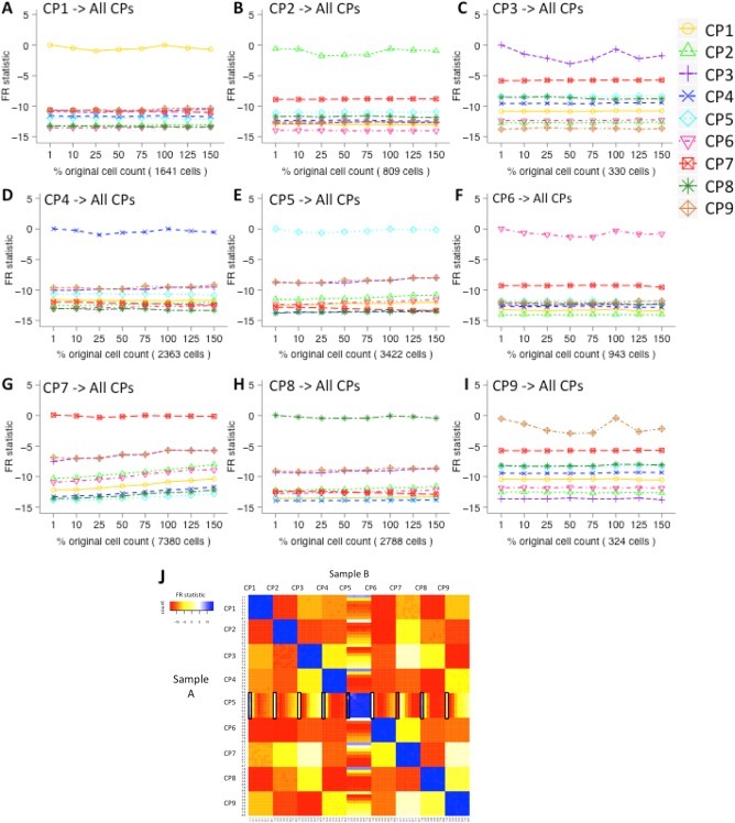
Matching cell populations that differ in proportions between samples. FR statistics comparing each simulated cell population CP1–CP9 (A–I, respectively) under varied proportions (1%, 10%, 25%, 50%, 75%, 100%, 125%, and 150% of the original cell count) with all cell populations in the reference sample containing 100% of all cell events. In all nine sets of analyses, the FR statistic is larger when comparing a changed cell population to the original cell population than when comparing it to the other cell populations across varying proportions of original cell counts. In other words, the changed cell population in the test sample can be determined to be most similar to the corresponding population in the reference sample based on the largest FR statistic value in a comparison against all nine populations in the reference sample. (J) Heat map for comparing all cell populations between the test samples (Sample Set A) and the reference samples (Sample Set B). We CP5 and changed its proportions in different test samples. The rows and columns are ordered by cell population IDs (CP1–CP9) and then by population proportion ID (1–8, with 1 being 1% and 8 being 150%). Squares colored in blue are the highly similar cell population pairs with an FR statistic close to 0, while yellow, orange, and red squares are more dissimilar pairs with negative FR statistics. The regions of the heat map that correspond to the comparisons displayed in parts A–I are indicated with rectangles. [Color figure can be viewed in the online issue, which is available at wileyonlinelibrary.com.]

We also compared cell populations across the test samples of CP5 changed proportions to demonstrate the utility of FR statistic in a multiple‐sample comparison scenario. In Figure 3J, a total of 72 × 72 FR statistics are displayed in a heat map (comparing 8 test samples of 9 cell populations) and listed in order of population proportions within each cell population block (e.g., CP5 block consists of 1% (#1.5), 10% (#2.5), 25% (#3.5), 50% (#4.5), 75% (#5.5), 100% (#6.5), 125% (#7.5), and 150% (#8.5)). The cell populations that were not changed in proportions are mapped to each other (i.e., FR statistics closer to zero) as expected. Although the 1% CP5 (#1.5) is slightly more similar to the other cell populations compared to the other changed CP5s, the 1% CP5 is still ranked as more similar to other CP5s under changed proportions than to any other cell population.

Matching with differences in cell population numbers between samples

In some cross‐sample comparison scenarios, differences in the numbers of cell populations detected in different samples might be expected. This could occur when comparing samples from normal healthy subjects with samples from diseased subjects in which a new abnormal cell population might be present (e.g., in leukemia or lymphoma patients, or in situations where stimulated and unstimulated samples are compared). Figure 3A–3I shows the estimated FR statistics for each population comparison. In this scenario, there would be no comparison for one of the cell populations (e.g., CP1) in the reference sample since that population has been removed from the test sample. Because the comparison performed by FlowMap‐FR occurs on a population‐by‐population basis, the FR statistic values for comparisons between the incorrect cell populations in the test sample and the extra population in the reference sample is essentially the same as if the extra population was still present in the test sample. Thus, for a missing CP1 population, all FR statistics values would correspond to a run value of 1 and the curves would be located at the bottom of the graph in the comparison depicted in Figure 3A. While all the correct pairwise comparisons would give FR statistic values close to 0 for eight out of eight comparisons, the extra population would only give low FR values (e.g., <−10 in most cases), similar to what is observed for incorrect comparisons. Thus, establishing a lower threshold of ∼−5 would indicate that any population without a value above −5 would indicate a unique population in one of the samples.

Matching with shifts in marker expression levels between samples

Shifts in marker expression between cell populations across a set of experimental samples can occur due to natural biological variability in genetically diverse populations, cell differentiation response to some perturbation, or technical variability associated with differences in staining procedures or reagent lots. In order to determine how the FR statistic would respond to shifts in marker expression, the nine cell populations were mapped to themselves and other cell populations in simulated scenarios in which one population (CP4) was shifted in position along each of the four dimensions. Shifting was standardized with respect to the range (IQR) of the cell populations’ distributions along the selected dimension (see Supporting Information Figure S3 for distributions of each CP). A total of 6 test samples were generated with shifting positions along each dimension. The results of CP4 mapping are shown in Figure 4; other results are shown in Supporting Information Figure S4A. The distribution of CP4 is narrow along CD19 and is wide along the other three dimensions. As the position shift increases along CD19 (with the distribution in all three other dimensions kept the same), the FR statistic for matching with the original CP4 initially drops linearly with the degree of shifting and then plateaus (Fig. 4A). Thus, FlowMap‐FR could be used to determine statistically meaningful shifts in marker expression within a cell population.

Figure 4.

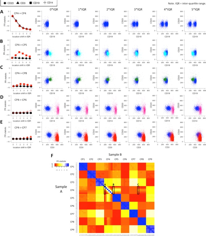
Matching cell populations with shifted marker distributions between samples. Shifted CP4 populations compared to the original (A) CP4 and (B–E) other unchanged cell populations. The amount of shifting is quantified as units of the calculated interquartile range (IQR) in each of the respective marker distributions (CD3, CD14, CD19, and CD23). The left‐most column displays the FR statistics for the five sets of population comparisons with CP4 shifts of 0, 1, 2, 3, 4, and 5 IQR units of the corresponding original marker distribution in the indicated dimension. In (A), the shifted CP4 is compared to itself. As the amount of shifting increases, the dissimilarity grows between the changed CP4 and the original CP4 as indicated by the increasingly negative FR statistic in the left‐hand graph. The FR statistics are similar along the four marker distributions. The red line highlights the comparisons with the most pronounced FR statistics change over IQR shifts. For example, in (E), the red line corresponds to the FR statistics for comparing shifted CP4 along the CD3 axis against CP7, and the three black lines correspond to the comparisons of CP4 against CP7 along the CD23, CD19, and CD14 axis. The dot plots shown to the right illustrate locations of CP7 and the shifted CP4 along the CD3 axis. (F) Heat map for comparing all cell populations between the test samples (Sample Set A) and the reference samples (Sample Set B). We chose CP4 and shifted it along the CD19 axis in the test samples. The rows and columns are ordered by cell population IDs (CP1–9) and then by population shift ID (1–6, with 1 being no shift and 6 being a 5×IQR shift). Squares colored in blue are the highly similar cell population pairs with an FR statistic close to 0, while yellow, orange, and red squares are more dissimilar pairs with negative FR statistics. The regions of the heat map that correspond to the comparisons displayed in parts A–C are indicated with rectangles. [Color figure can be viewed in the online issue, which is available at wileyonlinelibrary.com.]

In some cases, the shifted cell populations can also become more similar to other cell populations than to the corresponding population in the reference sample depending on the marker expression characteristics of the other populations. When CP4 is at a 2‐IQR unit shift away from the original position in the CD19 dimension, the FR value in comparison with itself in the reference sample is about −10 (Fig. 4A) and with CP5 is about −6 (Fig. 4B). This indicates that CP4 in the test sample has become more similar to CP5 in the reference sample at a 2‐unit shift. Indeed, the distribution of CP4 in the CD19 and CD23 dimensions overlaps closely with CP5 at a 2‐unit shift (see the scatter plots in Fig. 4B). However, even when substantial overlap was achieved between the shifted CP4 and the original CP5 at a 2‐unit shift along the CD19 dimension, the FR statistic was still below −5 due to differences in distributions between CP4 and CP5 in other dimensions. Similar observations were made for CP8 (Fig. 4C), which also overlaps with CP4 at 2‐unit shifts in the scatter plots. However, the comparison of CP8 with the shifted CP4 produced only a modest increase in the FR statistics to −11 since CP8 and CP4 are still quite different in shape and coverage of the feature space. Complete pairwise comparison results of the 6 CP4‐shifted samples are shown in Figure 4F. With respect to relative shifts of 0 or 1 IQR units, CP4s are more similar to themselves than to the other cell populations. The 3‐unit shift CP4 is more similar to the 2‐unit shift CP4, and the 4‐unit shift CP4 is more similar to the 3‐unit shift and 5‐unit shift CP4, and so on. We computed the P‐values of the FR statistic for the mapping of each cell population to its original parent cell population under shifts in marker expression levels. The results are shown in Supporting Information Figure S4B. The cutoff for P‐value was fixed at 10⁻⁷ across all three simulation cases. Similar to the FR statistics results shown in Supporting Information Figure S4A, −log 10 P‐values of the FR statistics increase linearly as the shift in marker position increases. Based on these results, using a P‐value threshold of 10⁻⁷ would generally provide robust mapping of populations with slight shifts (<1 IQR) in the expression of one of the cell surface markers between samples.

Matching with over‐partitioning of cell populations in some samples

During cell population identification, certain cell populations might be inappropriately divided into two (over‐partitioning) depending on the method and configuration parameters used, even though there is no real evidence that the two partitions correspond to distinct cell populations. In order to determine how FlowMap‐FR would handle over‐ and under‐partitioning, we artificially partitioned each of the nine cell populations above and below a range of selected percentiles along the CD23 expression level axis. A total of 18 test samples were generated for each cell population, consisting of its corresponding partitions (9 samples each for partitions above and below the percentile cutoffs, from 10% to 90%; see Methods for details); the other cell populations remained unchanged.

Figure 5A–5I shows the mapping results of the nine cell populations. (Corresponding bi‐axial distributions are shown in Supporting Information Fig. S5A–C.) In Figure 5A, the two sets of estimated FR statistics computed when mapping the two partitioned CP1s in the test sample to the unchanged CP1 in the reference sample are significantly larger than those obtained in comparison with the other cell populations. The test correctly mapped both partitioned cell populations to the unchanged reference cell population across varying partitions. Results also show that FR statistics increases when the partition size increases, so the two lines of FR statistics representing the two partitions cross as one partition increases size and the other decreases size. That the two lines are not completely symmetric is due to the nonsymmetric distribution of skew‐t data simulation. The same pattern is found for the other eight cell populations in Figure 5B–5I. Therefore, FlowMap‐FR is able to quantify similarity of inappropriately partitioned subpopulations with the original cell population in the reference sample and could therefore be used to detect and correct over‐partitioning that could arise from manual gating or algorithmic clustering. We also computed the P‐values of the FR statistics for each cell population comparison (Supporting Information Fig. S5D). Similar to the results of FR statistics, selecting a P‐value threshold of ∼10⁻⁷ distinguishes between correctly matched and incorrectly matched population partitions. Figure 5J displays the complete pairwise comparisons of CP5 partitions above cutoffs along CD23 expression levels with itself and other cell populations. From this heat map, it is clear that all 10 partitions of CP5 are more similar to the unpartitioned CP5 in the reference sample based on the FR statistic since all of the squares in the central CP5 vs CP5 box have a higher FR statistic (more blue) than any other comparisons of cell populations against CP5.

Figure 5.

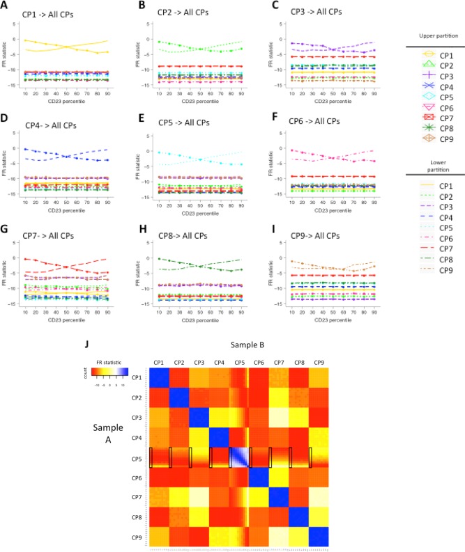
Matching cell populations inappropriately divided into two populations in one sample. (A–I) FR statistics comparing the two partitioned cell populations in the test sample to all (intact) cell populations in the reference sample. The two partitioned populations are generated by dividing the indicated cell population with a discrete value for CD23 marker expression so that the two partitioned populations are above and below the 10, 20, 30, 40, 50, 60, 70, 80, and 90^th percentile in the CD23 marker distribution. Across the analyses, the two intersecting lines seen at the top of each graph show that the FR statistics are always the largest when the two partitioned populations in the test sample are compared to the intact parent cell population in the reference sample. (J) Heat map for comparing all cell populations between the test samples (Sample Set A) and the reference samples (Sample Set B). We chose CP5 to partition and compared the 10 testing samples with different CP5 upper partitions along the CD23 axis with the intact CP5 in the reference samples. The rows and columns are ordered by cell population IDs (CP1–9) and then by partition ID (1–10, with 1 being 10^th percentile and 10 being no partition). Squares colored in blue are the highly similar cell population pairs with an FR statistic close to 0, while yellow, orange, and red squares are more dissimilar pairs with negative FR statistics. [Color figure can be viewed in the online issue, which is available at wileyonlinelibrary.com.]

Matching populations using the symmetric KL divergence (SKL) measure

Figure 6A–6I shows the results of matching CP1, CP2, and CP3 with all other cell populations using the SKL distance under scenarios in which differences in cell proportions occur between biological samples (A–C) and under scenarios in which a discrete cell population in one biological sample was inappropriately divided into two by over‐partitioning of the data from another biological sample (D–I). Corresponding results of CP4–CP9 are presented in Supporting Information Figure S6A–C. Under the scenario in which differences in cell proportions occur between biological samples, the SKL distance value is always close to zero when matching cell populations of varying proportions in the test sample to corresponding cell populations in the reference sample. However, the differences between the SKL distance values of equivalent and nonequivalent cell populations are not as large as those between the FR statistics (compare Fig. 6A–6C with Fig. 3). Thus, it could be difficult to use the SKL distance value to distinguish mapping from nonmapping cases. In theory, the SKL distance could be used for population mapping by choosing the best‐matched cell population. But if the cell population to be mapped does not occur in the test sample, mapping to the best‐matched population without considering the similarity value would give an incorrect result. Similar phenomena were found under scenarios in which a cell population is inappropriately divided into two by over‐partitioning (Fig. 6D–6I and Supporting Information Fig. S6B,C). The SKL distance performs poorly when comparing CP1 partitions below 10th, 20th, and 30th percentiles in the test sample with CP1 in the reference sample (Fig. 6D and 6G). In fact, the SKL distance values are smaller when comparing these CP1 partitions to CP4 in the reference sample than when comparing to the reference CP1.

Figure 6.

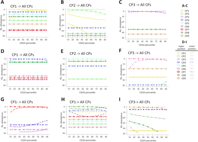
Matching cell populations using SKL divergence measure. (A–C) SKL distance values (y‐axis) from comparing CP1, CP2, and CP3 to all reference cell populations under varied proportions (x‐axis showing 1, 10, 25, 50, 75, 100, 125, and 150% of the original cell counts of CP1–3, compared against reference cell populations with 100% of their cell events). CP4–CP9 matching results can be found in Supporting Information Figure S6A. For example, in (A), each line records the eight SKL distance values generated from comparing eight different proportions of CP1 to each of the original cell populations, including itself. (D–I) The SKL distance of comparing two partitions of a cell population (CP1–3) to all reference cell populations, including itself. D–F display the SKL results in complete value ranges. G–I zoom in and show the top region of the D–F graphs with SKL values 0–50 so that the pattern of the lines can be seen. Results for CP4–CP9 have similar pattern and can be found in Supporting Information Figure S6B,C. [Color figure can be viewed in the online issue, which is available at wileyonlinelibrary.com.]

For scenarios in which cell populations are shifted in marker expression levels, the SKL distance performs in a similar way to the FR statistics, i.e., linearly changing values with increasing shifts. (The complete results can be found in Supporting Information Fig. S6D.)

Mapping Cell Populations Across Multiple Samples in Real Data

Real FCM data set #1

Figure 7A and 7B shows the results of matching cell populations across four real FCM samples using the FR‐based distance measure. Samples 1 and 2 are the biological replicates of the blood sample from the first subject, and Samples 3 and 4 are that of the second subject. In Figure 7A, the FR‐based distance measure (−1×FR statistic) was computed for each cell population pairwise comparison and displayed in a heat map. The blocks colored in blue suggest matched population pairs, and the blocks colored in red suggest mismatched population pairs. We employed hierarchical clustering method with complete linkage to match cell populations across samples, using the FR‐based dissimilarity measure as the distance metric. The cell populations were grouped into four sets of equivalent cell populations. For example, in the first set of matched cell populations, CP1.2 (Sample 1, CP 2), CP2.4 (Sample 2, CP4), CP4.3 (Sample 4, CP3), and CP3.4 (Sample 3, CP4) were grouped and matched to each other. CP1.2 and CP2.4 belong to biological replicates of one blood sample, while CP4.3 and CP3.4 belong to biological replicates of the other blood sample. In the hierarchical relationship of the cell populations across samples, CP1.2 is more similar to CP2.4 than to CP4.3 or to CP3.4. We observed the same relationship in each set of equivalent cell populations, namely that cell populations belonging to the biological replicates of the same sample are more similar to each other. Similar to the results of FR statistics, selecting a P‐value threshold of ∼10⁻⁷ also distinguishes between correctly matched and incorrectly matched populations. We also performed cell population mapping using flowMatch with the FR‐based distance measure and using flowMatch with symmetric KL divergence (SKL) as the distance measure. Both versions of flowMatch generated the same cell population mapping results as shown in Figure 7A. In Figure 7B, the hierarchical relationship between the samples was computed using flowMatch with the FR‐based distance measure. Supporting Information Figure S9 shows the flowMatch sample mapping results with both the SKL and FR distance measures. In both versions of flowMatch, biological replicates of the same blood sample are matched and more similar to each other than the FCM samples that come from different subjects.

Figure 7.

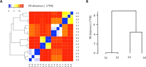
Matching cell populations across the real FCM data set #1. (A) Heat map of the FR distances (−1×FR statistics) for comparing all cell populations across four real flow cytometry samples. The cell populations in the samples were identified using K‐means clustering with possible number of cell populations ranging from 4 to 20. The FR statistics were computed for all possible pairwise comparison of the cell populations. We computed a dissimilarity measure based on the FR statistic (−1×FR) and employed the FR‐based distance measure to organize the cell populations using hierarchical clustering with complete linkage. (B) flowMatch results of matching FCM samples using the FR distance as the dissimilarity metric between cell populations across samples. The distance between FCM samples was computed based on the weighted sum of distance between cell populations across samples. y‐axis represents the FR‐based metric (−1×FR) between individual FCM samples. These results are the same as Figure 7A, where distance measure was only computed at the population level, and also the same as when applying the default flowMatch method with symmetric KL divergence measure as the distance metric (see Supporting Information Figure S9 and S10). [Color figure can be viewed in the online issue, which is available at wileyonlinelibrary.com.]

Real FCM data set #2

Figure 8 shows the results of matching cell populations across 30 real FCM samples using the FR‐based distance measure. The FR‐based distance measure was computed for each cell population pair comparison and displayed in a heat map. The blue blocks with large FR‐based distance (low FR statistic values) suggest matched population pairs, and the red blocks with small FR‐based distance (high FR statistic values) suggest mismatched population pairs. The cell populations are arranged in a hierarchy based on the FR similarity to all other cell populations. The cell populations were then grouped according to their FR distance as reflected in the structure of the hierarchical clustering tree to generate eight sets of equivalent cell populations. F‐measures were computed to evaluate the combined precision and recall of the FlowMap‐FR classification method. We obtained an overall F‐measure of 0.88, which indicates high agreement between manual gating/mapping and the cell population mapping derived from the FR‐based similarity matrix.

Figure 8.

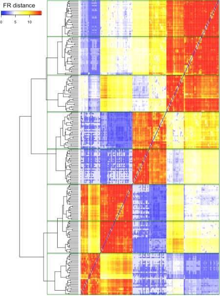
Matching cell populations across the real FCM data set #2. Heat map of the FR distance (−1×FR) for clustering all cell populations across 30 real flow cytometry samples in the real FCM data set #2. The FR statistics were computed for all 28,680 possible pairwise cell population comparisons. We multiplied the FR statistics by −1 to obtain a dissimilarity measure. Blue boxes in the dissimilarity heat map correspond to similar population pairs with small FR distance (large FR statistic); red box corresponds to population pairs that are not similar to each other with large FR distance (small FR statistic). Each sample had 8 cell populations delineated by expert manual gating as part of the FlowCAP‐I challenge. Cell populations are organized according to the value of the FR distance using hierarchical clustering with complete linkage. The green boxes on the plot delineate the eight cell populations deemed equivalent to each other across the 30 FCM samples in the experiment based on FR distance as reflected in the structure of the hierarchical clustering tree. [Color figure can be viewed in the online issue, which is available at wileyonlinelibrary.com.]

Discussion

Mapping of equivalent cell populations across different samples is an essential component of comparative analysis pipelines for cell‐based immunoprofiling and biomarker discovery in biomedical research to monitor disease progression and treatment responses. However, the ability to precisely match cell populations is complicated by natural and technical contributions to variation in marker expression values and their distributions. FlowMap‐FR directly addresses the cell population mapping challenges that may arise during the FCM data processing workflow without a priori assumptions about the marker expression distributions in the different cell populations analyzed, and thus can be readily employed in comparison of skewed, nonparametric, and multimodal distributions. The method is highly robust, as illustrated in matching cell populations of varying shapes, locations, and correlations between marker features under scenarios of differences in population proportions between samples and modest shifts in marker distributions. Because FlowMap‐FR is a stand‐alone cell population mapping method, it can be incorporated into any FCM analytical workflow that requires a cell population‐matching step.

The mapping approach in FlowMap‐FR provides a similarity measure of cell populations under various sample variation scenarios. This similarity measure can be converted into a probability measure assuming that the statistic follows a normal distribution 15. The statistic is an objective measure of similarity between data distributions, with values closer to zero reflecting similar data distributions (more precisely, that the two “samples” are derived from a single underlying global data distribution) and values approaching large negative values reflecting different data distributions (that the two “samples” are derived from different underlying global data distributions). However, the choice of whether two cell populations are “equivalent” is somewhat subjective and specific to the experiment in question. To deal with this experiment‐specific decision, it is possible to choose a threshold for the statistical value across the comparison pairs to distinguish equivalent (matched) versus distinct (mismatched) cell populations. We have observed larger gaps in the FR statistic values for threshold selection compared with other existing methods, such as the SKL distance. When cell population marker distributions were similar between samples, there was an obvious gap in the FR statistic values between matched versus mismatched cell population pairs such that the threshold was relatively easy to identify. Alternatively, an agglomerative clustering method, such as hierarchical clustering, could be applied to identify groupings of cell populations with similar expression profiles.

One challenging population mapping scenario occurs when one sample contains a cell population that is absent from another sample, as might occur when a novel abnormal cell population arises in a particular disease setting. We found that when there were different numbers of cell populations between the test and reference samples, judicious selection of an FR statistic threshold could reveal the presence of a distinct cell population in one sample that was absent from the other. However, the selection of this threshold could be challenging in some cases. In this scenario, the ideal reference sample for comparison would be one that contains the union of all cell populations found in each of the individual test samples. This composite sample could be generated by concatenating the data from multiple FCS files and running the population identification methods on the concatenated file to identify all cell populations present in each of the individual samples. This composite sample could then be used as a reference for comparison and mapping.

While FlowMap‐FR was relatively robust to moderate shifts in marker expression (<1 IQR) that could result from natural biological variability or differences in staining protocols/reagents and instrument configuration settings between experiments and labs, we expect that its performance could be enhanced further by applying a sample alignment procedure to the data before the population mapping step in the FCM data processing workflow. Cell populations observed can be similar in shape and relative location in each sample but different in absolute marker expression levels across samples. Marker expression levels can be normalized across samples on a per‐channel basis 25 before cell population mapping to further improve the results. Many software and computer programs are available for this data transformation purpose, such as flowTrans 13, FCSTrans (the method used in this article 22), FCS2CSV 26, and so on, before mapping cell populations in FlowMap‐FR.

However, in some experimental scenarios, marker expression shifts reflect important phenotypic changes in the cell population of interest, for example, when activation marker expression increases in response to cell stimulation. As a statistical test, FlowMap‐FR can be used to determine when the expression of a cellular marker has become significantly different from a comparison population (e.g., using FR values from known different cell types in control samples to determine thresholds). Although the FR statistic cannot determine whether one cell population is functionally different from the other, it provides an objective measure for scientists to identify candidate phenotypes for biological interpretation and validation.

FlowMap‐FR was also found to be able to map cell populations that are inappropriately partitioned in a subset of samples. We observed that across varying partitions of cell populations in different samples, FlowMap‐FR correctly mapped the partitions to the original cell populations in the reference sample and ranked the partitions by degree of overlap with respect to the original cell population. The over‐ or under‐partitioning of cell populations is a common artifact in many automatic gating methods. Thus, the FR statistic can also serve as a tuning metric for parameter adjustment during the automated gating process to prevent artificial population splitting or simply as a quality control metric on the gated samples.

Computational efficiency is a major consideration in the analytical workflow of FCM data processing because of the increasingly large quantities of samples, events, and markers being evaluated. The bottleneck of FlowMap‐FR computations lies in finding the minimum spanning tree (MST) in order to compute the FR statistic. We used Prim's algorithm to compute the MST, in which the computational complexity increases quadratically in the number of nodes, i.e., the number of events in the graph (see Supporting Information Fig. S7A,B). To circumvent the runtime limitation, we implemented a controlled random sampling procedure to estimate the FR statistic for each cell population pair comparison. The random sample procedure achieved good precision and accuracy in estimating the true FR statistic (see Supporting Information Fig. S8A,B). Moreover, we parallelized the estimation procedure so that the users may choose to perform the analysis on as many cores as their computing environment allows. For a single‐cell population comparison in FCM samples with four feature markers, the runtime on a 10 core system is ∼10 times faster than the run time on a single core system (see Supporting Information Methods for more details). In the future, the runtime can be further improved by parallelizing the sequential computations of multiple sample comparison of cell populations.

We have implemented FlowMap‐FR in R as a Bioconductor package (http://www.bioconductor.org/packages/devel/bioc/html/flowMap.html). We are also in the process of implementing and incorporating FlowMap‐FR into the GenePattern FCM suite 27 and the bioKepler workflow platform 28, so that it can be used along with other FCM data processing and analytical methods that have been deployed in these platforms. A common FCM computational workflow consists of four steps: data transformation and preprocessing, computational identification of cell populations, sample alignment, and cross‐sample comparison of cell populations. While there have been a large number of methods developed for the transformation and identification steps, only a few methods are available for the sample alignment and cross‐sample comparison steps. FlowMap‐FR provides a robust nonparametric probability‐based solution to these workflows, facilitating the move toward the next paradigm for result interpretation across samples and objective performance evaluation of workflows.

Supporting information

Supporting Information

Supporting Information

Literature Cited

- 1. Mellman I, Coukos G, Dranoff G. Cancer immunotherapy comes of age. Nature 2011;480(7378):480–489. [DOI] [PMC free article] [PubMed] [Google Scholar]
- 2. Chattopadhyay P, Perfetto S, Gaylord B, Stall A, Duckett L, Hill J, Nguyen R, Ambrozak D, Balderas R, Roederer M. “Toward 40+ Parameter Flow Cytometry,” in CYTO Conference Plenary Presentation and Abstract 388, 2014.
- 3. Akdis CA, Akdis M. Mechanisms and treatment of allergic disease in the big picture of regulatory T cells. J Allergy Clin Immunol 2009;123(4):735–746; quiz 747–748. [DOI] [PubMed] [Google Scholar]
- 4. Casale TB, Busse WW, Kline JN, Ballas ZK, Moss MH, Townley RG, Mokhtarani M, Seyfert‐Margolis V, Asare A, Bateman K, Deniz Y. Omalizumab pretreatment decreases acute reactions after rush immunotherapy for ragweed‐induced seasonal allergic rhinitis. J Allergy Clin Immunol 2006;117(1):134–140. [DOI] [PubMed] [Google Scholar]
- 5. Aghaeepour N, Finak G, Hoos H, Mosmann TR, Brinkman R, Gottardo R, Scheuermann RH. Critical assessment of automated flow cytometry data analysis techniques. Nat Methods 2013;10(3):228–238. [DOI] [PMC free article] [PubMed] [Google Scholar]
- 6. Cron A, Gouttefangeas C, Frelinger J, Lin L, Singh SK, Britten CM, Welters MJP, van der Burg SH, West M, Chan C. Hierarchical modeling for rare event detection and cell subset alignment across flow cytometry samples. PLoS Comput Biol 2013;9(7):e1003130. [DOI] [PMC free article] [PubMed] [Google Scholar]
- 7. Pyne S, Hu X, Wang K, Rossin E, Lin T‐I, Maier LM, Baecher‐Allan C, McLachlan GJ, Tamayo P, Hafler DA, De Jager PL, Mesirov JP. Automated high‐dimensional flow cytometric data analysis. Proc Natl Acad Sci USA 2009;106(21):8519–8524. [DOI] [PMC free article] [PubMed] [Google Scholar]
- 8. Lo K, Brinkman RR, Gottardo R. Automated gating of flow cytometry data via robust model‐based clustering. Cytometry Part A 2008;73A(4):321–332. [DOI] [PubMed] [Google Scholar]
- 9. Pyne S, Lee SX, Wang K, Irish J, Tamayo P, Nazaire M‐D, Duong T, Ng S‐K, Hafler D, Levy R, Nolan GP, Mesirov J, McLachlan GJ. Joint modeling and registration of cell populations in cohorts of high‐dimensional flow cytometric data. PLoS One 2014;9(7):e100334. [DOI] [PMC free article] [PubMed] [Google Scholar]
- 10. Qian Y, Wei C, Eun‐Hyung Lee F, Campbell J, Halliley J, Lee JA, Cai J, Kong YM, Sadat E, Thomson E, Dunn P, Seegmiller AC, Karandikar NJ, Tipton CM, Mosmann T, Sanz I, Scheuermann RH. Elucidation of seventeen human peripheral blood B‐cell subsets and quantification of the tetanus response using a density‐based method for the automated identification of cell populations in multidimensional flow cytometry data. Cytometry Part B Clin Cytom 2010;78B(Suppl 1):S69–S82. [DOI] [PMC free article] [PubMed] [Google Scholar]
- 11. Zare H, Shooshtari P, Gupta A, Brinkman RR. Data reduction for spectral clustering to analyze high throughput flow cytometry data. BMC Bioinformatics 2010;11:403. [DOI] [PMC free article] [PubMed] [Google Scholar]
- 12. Roederer M, Moore W, Treister A, Hardy RR, Herzenberg LA. Probability binning comparison: A metric for quantitating multivariate distribution differences. Cytometry 2001;45:47–55. [DOI] [PubMed] [Google Scholar]
- 13. Finak G, Perez J‐M, Weng A, Gottardo R. Optimizing transformations for automated, high throughput analysis of flow cytometry data. BMC Bioinformatics 2010;11(1):546. [DOI] [PMC free article] [PubMed] [Google Scholar]
- 14. Azad A, Pyne S, Pothen A. Matching phosphorylation response patterns of antigen‐receptor‐stimulated T cells via flow cytometry. BMC Bioinformatics 2012;13(Suppl 2):S10. [DOI] [PMC free article] [PubMed] [Google Scholar]
- 15. Friedman JH, Rafsky LC. Multivariate generalizations of the Wald–Wolfowitz and Smirnov two‐sample tests. Ann Stat 1979;7(4):697–717. [Google Scholar]
- 16. Zhao Ti, Soto S, Murphy RF. Improved comparison of protein subcellar location patterns. In 3rd IEEE international Symposium on Biomedical Imaging: Nano to Marco; 2006:562–565.
- 17. Theoharatos C, Laskaris N, Economou G, Fotopoulos S. A generic scheme for color image retrieval based on the multivariate Wald–Wolfowitz test. IEEE Trans Knowledge Data Eng 2005;17(6):808–819. [Google Scholar]
- 18. Neemuchwala H, Zabuawala HAS, Carson P. Image registration methods in high dimensional space. Int J Imaging Syst Technol 2007;16(5):130–145. [Google Scholar]
- 19. Wald A. Wolfowitz J. An exact test for randomness in the non‐parametric case based on serial correlation. Ann Math Stat 1943;14(4):378–388. [Google Scholar]
- 20. Moret BME, Shapiro HD. An empirical analysis of algorithms tree,” in Algorithms and Data Structure, Lecture Notes in Computer Science Volume 519, 1991:400–411. [Google Scholar]
- 21. Prim R. Shortest connection networks and some generalizations. Bell Syst Tech J 1957;36(6):1398–1401. [Google Scholar]
- 22. Qian Y, Liu Y, Campbell J, Thomson E, Kong YM, Scheuermann RH. FCSTrans: An open source software system for FCS file conversion and data transformation. Cytometry Part A 2012;81A(5):353–356. [DOI] [PMC free article] [PubMed] [Google Scholar]
- 23. Klunker S, Saggar LR, Seyfert‐Margolis V, Asare AL, Casale TB, Durham SR, Francis JN. Combination treatment with omalizumab and rush immunotherapy for ragweed‐induced allergic rhinitis: Inhibition of IgE‐facilitated allergen binding. J Allergy Clin Immunol 2007;120(3):688–695. [DOI] [PubMed] [Google Scholar]
- 24. Azad A. healthyFlowData : Healthy dataset used by the flowMatch package. R package version 1.3.1; 2013.
- 25. Lo K, Hahne F, Brinkman RR, Gottardo R. flowClust: A bioconductor package for automated gating of flow cytometry data. BMC Bioinformatics 2009;10:145. [DOI] [PMC free article] [PubMed] [Google Scholar]
- 26. http://sourceforge.net/projects/flowcyt/files/GenePattern Flow Cytometry Suite/FCS2 CSV/. Accessed February 02, 2012.
- 27. Spidlen J, Barsky A, Breuer K, Carr P, Nazaire M‐D, Hill BA, Qian Y, Liefeld T, Reich M, Mesirov JP, Wilkinson P, Scheuermann RH, Sekaly R‐P, Brinkman RR. GenePattern flow cytometry suite. Source Code Biol Med 2013;8:1–8. [DOI] [PMC free article] [PubMed] [Google Scholar]
- 28. Altintas I. Distributed workflow‐driven analysis of large‐scale biological data using biokepler, Proc. 2nd Int. Work. Petascal data Anal. challenges Oppor.—PDAC’11, p. 41, 2011.
Associated Data
This section collects any data citations, data availability statements, or supplementary materials included in this article.
Supplementary Materials