An assessment of phytoplankton primary productivity in the Arctic Ocean from satellite ocean color/in situ chlorophyll‐a based models

Abstract

We investigated 32 net primary productivity (NPP) models by assessing skills to reproduce integrated NPP in the Arctic Ocean. The models were provided with two sources each of surface chlorophyll‐a concentration (chlorophyll), photosynthetically available radiation (PAR), sea surface temperature (SST), and mixed‐layer depth (MLD). The models were most sensitive to uncertainties in surface chlorophyll, generally performing better with in situ chlorophyll than with satellite‐derived values. They were much less sensitive to uncertainties in PAR, SST, and MLD, possibly due to relatively narrow ranges of input data and/or relatively little difference between input data sources. Regardless of type or complexity, most of the models were not able to fully reproduce the variability of in situ NPP, whereas some of them exhibited almost no bias (i.e., reproduced the mean of in situ NPP). The models performed relatively well in low‐productivity seasons as well as in sea ice‐covered/deep‐water regions. Depth‐resolved models correlated more with in situ NPP than other model types, but had a greater tendency to overestimate mean NPP whereas absorption‐based models exhibited the lowest bias associated with weaker correlation. The models performed better when a subsurface chlorophyll‐a maximum (SCM) was absent. As a group, the models overestimated mean NPP, however this was partly offset by some models underestimating NPP when a SCM was present. Our study suggests that NPP models need to be carefully tuned for the Arctic Ocean because most of the models performing relatively well were those that used Arctic‐relevant parameters.

Key Points

• The models reproduced primary productivity better using in situ chlorophyll‐a than satellite values

• The models performed well in low‐productivity seasons and in sea ice‐covered/deep‐water regions

• Net primary productivity models need to be carefully tuned for the Arctic Ocean

1. Introduction

Model estimates of net primary production (NPP) that are inclusive of the Arctic Ocean (AO) are now available or coming online, ranging from simpler ones that largely address phytoplankton physiology or phytoplankton‐zooplankton coupling, to general circulation models that simulate the AO circulation, including sea ice, and that now incorporate biogeochemistry, food webs, and, in some cases, even sea‐ice algae. Given the high heterogeneity of the AO with its marginal seas and the rapid change the AO is undergoing, models are the best tool we have to simulate current conditions, reproduce historical observations, and project future conditions of NPP in the AO.

The AO remains one of the most undersampled of the world's oceans. This results from the unique combination of (a) inhospitable field conditions that prevent large‐scale, sustained sampling, (b) the presence of sea ice and its variability, (c) 6 months of relative darkness, (d) rapid seasonal changes in pan‐Arctic climate, (e) inter‐annual changes of the AO system, and (f) the complexity of the physical‐biological interactions of the marine Arctic ecosystem. These factors, coupled with a diplomatic lack of access to major portions of the AO, have resulted in a scarcity of extensive and/or continuous field data/programs. Hence, satellite‐measured ocean color provides a highly valuable data set with which NPP can be derived in the remote and often inhospitable AO, allowing for more extensive spatial coverage of the ocean surface, at least during the periods with sufficient solar elevations. However, satellite‐derived ocean‐color products are still prone to large uncertainties in polar regions due to conditions specific to these environments, such as low solar elevation and sea ice [IOCCG, 2015].

The seasonal cycle of primary production in the AO has been characterized by the classic pattern of a large pulse of growth in spring, sometimes followed by a smaller one in late summer/early fall [Sakshaug, 2004]. The traditional controls by light (onset of the phytoplankton bloom early on) and nutrients (magnitude of NPP later in the season) are further dependent in the AO on feedbacks with the cryosphere and the atmosphere. Light availability and water column stability change as the sea ice recedes northward, resulting in the phytoplankton bloom that occurs along an ice‐edge [Alexander and Neibauer, 1981; Perrette et al., 2011] or that may even be widespread underneath the ice [Sakshaug et al., 1991; Mundy et al., 2009; Arrigo et al., 2014]. Coastal inputs of fresh water affect both the stability and the transparency of the upper water column differently in various regions. In regions near sea‐ice, NPP is usually highest at the surface, which is likely due to the bloom being at its initial stage there, regardless of month [Wassmann, 2011]. Later in the growth season, deep maxima of phytoplankton chlorophyll‐a develop in seasonally ice‐free shelf regions [Brown et al., 2015] and in the central Arctic Basin where a strong halocline limits winter mixing [Tremblay et al., 2008 ; Ardyna et al., 2013]. Consequently, NPP in the AO is strongly modulated by stratification and circulation features controlled by the presence or absence of sea ice, ultimately enhancing or constraining nutrient supply and light exposure of phytoplankton [McLaughlin and Carmack, 2010]. Snow and ice cover also determine the amount of photosynthetically available radiation (PAR) in the upper part of the AO water column. Increased light penetration due to anticipated reductions in snow/ice cover may, however, only modestly increase NPP [Codispoti et al., 2013; Tremblay and Gagnon, 2009], because nutrient supply is low in certain AO regions [Carmack, 2007] or in the shallow summertime mixed layer. Using ocean color models, others propose that the increasing fraction of open water and higher availability of incoming radiation result in increased pan‐Arctic NPP, though regionally varying [Arrigo and van Dijken, 2011; Bélanger et al., 2013; Pabi et al., 2008], an earlier onset of phytoplankton blooms [Kahru et al., 2010], and the development of a persistent fall bloom [Ardyna et al., 2014].

Reliable models that estimate NPP, including both ocean color models (OCMs) and global/regional biogeochemical ocean general circulation models (BOGCMs), are becoming increasingly available for the AO and can help us better understand how NPP is changing, and how such changes are impacting this marine ecosystem. However, both types of models are associated with a substantial degree of uncertainty [Babin et al., 2015]. While the total, annual integrated NPP computed from BOGCMs may be of similar magnitude, the processes involved and their relative importance are very different in various model formulations [e.g., Popova et al., 2012; Vancoppenolle et al., 2013; Zhang et al., 2010]. In particular, BOGCMs are highly dependent on a realistic representation of ocean physics, specifically vertical mixing, which is one of the main mechanisms supplying inorganic nutrients to the AO surface waters [Popova et al., 2012].

Ocean color NPP models are also challenged in the AO due to the often simultaneous occurrence of sea‐ice presence during the growth season, a subsurface chlorophyll‐a maximum (SCM; often referred to as a deep chlorophyll‐a maximum), and enhanced coastal turbidity [IOCCG, 2015]. Furthermore, the extensive presence of clouds in summer [Eastman and Warren, 2010; Intrieri et al., 2002] and the lack of light in winter limit the period of observation. As a result, until recently we have not had sufficient spatial and temporal in situ data coverage to evaluate trends and variability of satellite‐derived NPP over the entire AO. Historically, the scarcity of in situ data for validation has affected our ability to accurately simulate contemporary mean NPP and its variability in the AO [Wassmann and Reigstad, 2011]; however, a recent data compilation [Hill et al., 2013; Matrai et al., 2013; Codispoti et al., 2013] including historical NPP, chlorophyll‐a concentration (hereafter chlorophyll), and nutrient data (1954–2007), as well as recent in situ data collected during the International Polar Year (2007–2008) are now available, together with data from more recent polar research field campaigns during 2009–2011. These data sets allow validation and calibration of OCMs and BOGCMs in the AO, as well as the testing of multiple ecological hypotheses [e.g., Ardyna et al., 2013; Arrigo et al., 2011].

In order to better understand the strengths and limitations of currently available NPP estimates for the AO, we conducted a Primary Productivity Algorithm Round Robin (PPARR) activity to assess the skill and sensitivity of NPP models in the AO. This study is based on multiple ocean color models using input fields from a combination of in situ, reanalysis, and satellite data. Our goal is to help inform the scientific community regarding model selection for the AO ecosystem and to identify the primary drivers of NPP model uncertainty. Given the high sensitivity of the AO under a changing climate, our NPP modeling assessment also provides an essential step forward to advance our knowledge of the observed contemporary changes in this region, which is crucial to understanding a key uncertainty in future climate projections.

2. Previous PPARR Activities

Since the launch of the Sea‐viewing Wide Field‐of‐view Sensor (SeaWiFS) in 1997, a number of PPARR activities have been conducted to assess the feasibility of estimating primary productivity from space‐based observations. The earliest PPARR exercises compared in situ uptake rates of isotopically labeled carbon (¹⁴C) with NPP estimated from satellite algorithms; they were applied to only a few regions that accounted for a very small sample size of measurements (<100) and found systematic offsets between them [Campbell et al., 2002]. The more recent PPARR studies (PPARR3 and PPARR4) have differed from the earlier ones by including not only ocean color‐based NPP models, but also BOGCMs as well. In the first stage of PPARR3, integrated NPP outputs from ∼20 models were compared (model‐model comparisons), global and regional deviations were identified, and a sensitivity study was performed to identify model‐specific sensitivities to the input variables [Carr et al., 2006]. This was followed by an evaluation of model skill in ∼30 models (model‐in situ data comparisons), and specifically focused on a large, quality‐controlled database (∼1000 measurements) from the tropical Pacific [Friedrichs et al., 2009]. By examining uncertainties associated with the input variables (e.g., surface chlorophyll, PAR, and SST), it was determined that more than half of the model‐data NPP differences could be accounted for by errors/uncertainties in these input variables. The PPARR4 study expanded these comparisons with in situ data in key regions critical for NPP models such as coastal waters, the oligotrophic subtropics, and the Southern Ocean [Saba et al., 2010, 2011]. These previous PPARR studies revealed that ocean color model skill was lowest in coastal waters where NPP was typically overestimated. Model estimates of NPP in pelagic waters were closer to those derived from ¹⁴C estimates, but, in general, these model values underestimated observations. Although these most recent PPARR studies included model skill comparisons in the high latitude Southern Ocean, the AO was not included.

3. Data and Methods

We assembled a quality‐controlled in situ database that includes a set of productivity‐related variables at 455 stations sampled mostly in the Chukchi, Beaufort, Barents, and Nordic Seas, and the Canadian Archipelago from 1988 to 2011 (Figure 1a). This database was built upon the ARCSS‐PP data set [Matrai et al., 2013], available at NOAA/National Oceanographic Data Center (NODC) (http://www.nodc.noaa.gov/cgi-bin/OAS/prd/accession/details/63065), and was supplemented with more recent international polar research activities (Table 1). Also, daily sea ice concentration at each sampling station was determined using NOAA/National Snow and Ice Data Center (NSIDC) Climate Data Record of Passive Microwave Sea Ice Concentration, Version 2 [Meier et al., 2013]. Roughly half of the stations (47%) were sampled in ice‐free regions (sea ice concentration < 15%, a threshold to determine sea ice extent used by NOAA/NSIDC) (Figure 1b).

Figure 1.

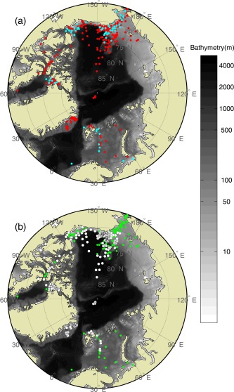
The total number of N=455 sampling stations (1988–2011) where in situ chlorophyll, SST, MLD and integrated NPP are available: (a) the blue circles (N=85) represent the subset stations where matchups between in situ station and satellite data exist, and (b) the green circles are the sampling stations (N=212) from ice‐free regions (sea ice concentration < 15%) and the white circles (N=243) are the sampling stations from ice‐covered regions (sea ice concentration ≥ 15%).

Table 1.

Description of the Field Program/Expedition/Database/Contributor Where NPP Data Were Obtained and Used for This Study^a

Year	Program/Expedition/Database/Contributor	Number of Stations	Season	Region	Reference/Investigator/Website
1988	AOOS	9	Jun–Sep	4	b
1992	OPPWG	32	Jul–Aug	6	b
1993	V. Hill	9	Aug	2, 4	b
1995	V. Hill	5	Aug	6	b
1996	V. Hill	2	Aug	6	b
1997	Vedernikov and Gagarin	6	Sep–Oct	6	Vedernikov and Gagarin [1998]
1998	ALV	4	Mar, May	6	Matrai et al. [2007]
	Vedernikov et al.	3	Aug	6	Vedernikov et al. [2001]
	NOW	32	Apr–Jul	3	Klein et al. [2002]
1999	ALV	4	Jul	6	Matrai et al. [2007]
	NOW	10	Aug–Sep	3	Klein et al. [2002]
2000	V. Hill	10	Aug	2, 4	b
2001	AOE	6	Jul–Aug	1	Olli et al. [2007]
2002	SBI	42	May–Aug	2, 4	Hill et al. [2005]
2003	CASES	5	Sep–Nov	2, 3	Brugel et al. [2009]; Tremblay et al. [2011]
2004	CABANERA	3	Jul	6	Hodal and Kristiansen [2008]
	CASES	11	Jun–Jul	2, 3	Brugel et al. [2009]; Tremblay et al. [2011]
	SBI	43	Jun–Aug	2, 4	Hill et al. [2005]
2005	CABANERA	1	May	6	Hodal and Kristiansen [2008]
	ArcticNet	12	Aug–Sep	2, 3	Lapoussière et al. [2009]; Ardyna et al. [2011]; Ferland et al. [2011]
2006	ArcticNet	11	Sep–Oct	2, 3	Ardyna et al. [2011]; Ferland et al. [2011]
2007	ArcticNet	5	Sep–Oct	3	Ardyna et al. [2011]
	Oshoro‐Maru	7	Aug	4	S. H. Lee (personal communication, 2014)
2008	ArcticNet	7	Sep	3	M. Gosselin (personal communication, 2014)
	ICE‐CHASER	5	Jul–Aug	6	Charalampopoulou et al. [2011]
	CFL	9	Jun–Aug	2, 3	Mundy et al. [2009]; Sallon et al. [2011]
	CHINARE	20	Aug–Sep	1, 2, 4	S. H. Lee (personal communication, 2014)
2009	Malina	22	Jul–Aug	2	http://malina.obs-vlfr.fr/
	JAMSTEC	13	Sep–Oct	1, 2, 4	http://www.godac.jamstec.go.jp/darwin/e/
	RUSALCA	18	Sep	1, 4, 5	S. H. Lee (personal communication, 2014)
	JOIS	10	Sep–Oct	1, 2	Yun et al. [2012]
2010	ArcticNet	7	Aug–Oct	3	M. Gosselin (personal communication, 2014)
	KOPRI	11	Jul–Aug	1, 4	S. H. Lee (personal communication, 2014)
	ICESCAPE	24	Jun–Jul	4	http://seabass.gsfc.nasa.gov/; Arrigo et al. [2014]
	JAMSTEC	2	Oct	1, 4	http://www.godac.jamstec.go.jp/darwin/e/
2011	ArcticNet	12	Jul–Oct	2,3	M. Gosselin (personal communication, 2014)
	ICESCAPE	23	Jun–Jul	4	http://seabass.gsfc.nasa.gov/; Arrigo et al. [2014]

The data from the ARCSS‐PP database [Matrai et al., 2013] are italicized and sub‐Arctic regions are labeled as following: 1––Arctic Basin, 2––Beaufort Sea, 3––Canadian Archipelago including Baffin Bay, 4––Chukchi Sea, 5––East Siberian Sea, and 6––Nordic Seas (Greenland and Barents Sea).

See ARCSS‐PP database for further details.

3.1. In Situ Net Primary Productivity

The 455 stations (Table 1) were chosen such that (1) NPP measurements, using ¹³C‐ or ¹⁴C‐labeled compounds, were available at four or more different depths, (2) the minimum sampling depth of NPP was between 0 and 5 m depth, and (3) additional in situ data were available including surface chlorophyll, sea surface temperature (SST) and mixed layer depth (MLD). Most in situ NPP using a ¹⁴C label (N=324) were measured after 24 h in situ or simulated in situ incubations and the rest of the ¹⁴C data (N=50) were measured after less than a 12 h incubation or an unknown time period; most data were reported as daily values. In situ carbon uptake rates using a ¹³C label (N=81) were measured after 3–6 h on‐deck incubations [Lee and Whitledge, 2005; Lee et al., 2010]; a good agreement between estimates of ¹³C and ¹⁴C productivity has been reported [Cota et al., 1996]. If hourly in situ production rates were reported, they were converted to daily production rates by multiplying with a calculated day length [Forsythe et al., 1995], based on the date and latitude when/where each sample was taken.

Using the multiple segment trapezoidal rule, NPP was integrated from the surface (Z₀) to the euphotic depth (Z_eu; 1% surface PAR) that was already determined during the incubation in most of the data. If Z_eu was not reported, then it was calculated from available light penetration data. Prior to any integration, if the NPP value at Z₀ was not measured, it was assumed to be the same as the closest measurement taken from the uppermost 5m (Z_min) of the water column in each station. Analogously, if Z_eu was deeper than the maximum sampling depth (Z_max), NPP at Z_eu was assumed to be the same as that measured at Z_max; (1) if NPP at Z_max was less than 1.0 mgC m⁻³ d⁻¹ (the 25^th percentile value among the available measurements of in situ NPP) or (2) if the distance between Z_max and Z_eu was less than 1 m. If Z_eu was shallower than Z_max, NPP at Z_eu was linearly interpolated.

The majority of the 455 NPP samples were collected from the region between 65 and 89°N mainly from late spring to early fall, and were characterized by significant spatial and temporal variability (Figure 2). The lowest integrated NPP (1.4 mgC m⁻² d⁻¹) was observed in the Beaufort Sea in October 2009 and the highest NPP (10,317 mgC m⁻² d⁻¹) was observed in the Chukchi Sea in July 2004. The median of the NPP at the 455 stations (NPP_N=455) was 214 mgC m⁻² d⁻¹. Integrated NPP exhibited a log‐normal distribution (Figure 2a) that was tested with the Kolmogorov‐Smirnov (K‐S) test (not shown). The NPP data were log‐transformed (base 10) [Campbell, 1995] before being analyzed in this study. The mean log‐transformed NPP_N=455 was 2.33 and the standard deviation was 0.72 (Table 2).

Figure 2.

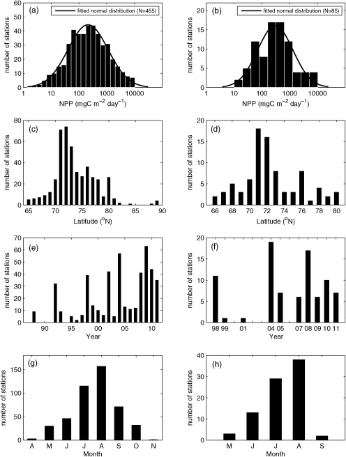
(left) In situ integrated NPP at the N=455 in situ sampling stations and (right) from the N=85 satellite matchup stations shown in Figure 1. Figures 2a and 2b are the distribution of in situ integrated NPP. Figures 2c and 2d, Figures 2e and 2f, and Figures 2g and 2h show where and when those in situ NPP were measured in terms of latitude, year, and month, respectively.

Table 2.

Mean (μ) and Standard Deviation (σ) of In Situ logNPP at the 455 Stations (1988–2011; N=455) and the 85 Stations (1998–2011; N=85) in Different Months and Regions^a

Months/Regions	Period: 1988–2011 (N=455)				Period: 1998–2011 (N=85)
	N	logNPP (μ±σ)	NPP (mgC m−2 d−1)		N	logNPP (μ±σ)	NPP (mgC m−2 d−1)
			10μ	95% CI [10μ − 1.96σ; 10μ+1.96σ]			10μ	95% CI [10μ − 1.96σ; 10μ+1.96σ]
Apr–Jun	79	2.66 ± 0.63	425	[21; 8493]	16	2.89 ± 0.50	782	[83: 7361]
Jul	115	2.65 ± 0.67	442	[21; 9212]	29	2.74 ± 0.56	554	[44; 6904]
Aug	127	2.27 ± 0.64	187	[10; 3415]	38	2.14 ± 0.54	137	[12; 1557]
Sep–Nov	104	1.84 ± 0.61	70	[4; 1123]	2	2.10 ± 0.43	125	[18; 877]
Shallow (≤200 m)	195	2.57 ± 0.72	375	[15; 9681]	38	2.69 ± 0.65	495	[26; 9300]
Deep (>200 m)	260	2.15 ± 0.66	140	[7; 2769]	47	2.32 ± 0.56	207	[16; 2617]
Sea ice‐free (<15%)	212	2.32 ± 0.65	207	[11; 3946]
Sea ice‐covered (≥15%)	243	2.34 ± 0.77	220	[7; 7235]
Total	455	2.33 ± 0.72	214	[8; 5481]	85	2.48 ± 0.63	305	[18; 5292]

μ and 95% confidence interval (CI; μ±1.96σ) are inverse‐transformed to the original scale (mg C m⁻² d⁻¹). The gray shading indicates no values.

The subset of stations used in most of our analyses is less than 20% of the total (N=85), because this model skill assessment was based on algorithms using satellite data that were only available after 1997 and that also had in situ match ups in sea ice‐free regions. For this subset of the data, NPP was measured mostly during July–August (Figure 2h) from 1998 to 2011 (Figure 2f), primarily in the region between 66°N and 80°N (Figure 2d). The in situ NPP at the 85 stations (NPP_N=85) ranged from as low as 10 mgC m⁻² d⁻¹ in Baffin Bay (September 1999) to as high as 10,317 mg C m⁻² d⁻¹ in the Chukchi Sea (July 2004), again exhibiting a log‐normal distribution (Figure 2b) with the median NPP being 305 mgC m⁻² d⁻¹. The mean log‐transformed NPP_N=85 was 2.48 and the standard deviation was 0.63 (Table 2).

The two data sets described above (NPP_N=455 and NPP_N=85) were compared using the K‐S two‐sample test which failed to reject the null hypothesis with a 5% significance level (not shown). This indicates that the two data sets are not statistically different and could be drawn from the same population with equal mean and variance (Figure 3a).

Figure 3.

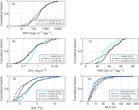
Cumulative distribution functions of integrated NPP and the various input variables for the full data set (N=455) and the data subset (N=85). (a) In situ logNPP, (b) in situ and satellite chlorophyll (CHL), (c) satellite and reanalysis PAR, (d) in situ and reanalysis SST, and (e) in situ and climatological MLD.

3.2. Input Variables

The majority of NPP models participating in this comparison exercise required a variety of input data fields, including surface chlorophyll, PAR, SST, and MLD (Table 3). In order to test the sensitivity of the models to the input data provided, two sources of data were provided to the modeling teams for each of the primary input variables: chlorophyll (in situ and satellite), PAR (reanalysis and satellite), SST (in situ and reanalysis), and MLD (in situ and climatology). In addition, other satellite‐derived properties (e.g., remote sensing reflectance, total/phytoplankton absorption coefficient, and particulate backscattering coefficient) required by some of the participating models were provided (Table 3).

Table 3.

Contributed Ocean Color Models^a

Model	Contributor(s)	Type	Input Variables					Reference
			CHL	PAR	SST	MLD	Remotely Sensed
1	D. Antoine and B. Gentili	DR,WR	•	•	•	•		Morel [ 1991]; Antoine and Morel [ 1996]; Antoine et al. [ 1996]; Morel et al. [ 1996]
2	F. Mélin	DR,WR	•	•				Mélin [ 2003]; Mélin and Hoepffner [ 2011]
3	F. Mélin	DR,WR	•	•			Rrs	Mélin [ 2003]; Mélin and Hoepffner [ 2011]
4	F. Mélin	DR,WR	•	•				Mélin [ 2003]; Mélin and Hoepffner [ 2011]
5	K. Waters	DR,WR	•	•	•	•		Ondrusek et al. [ 2001]
6	K. Waters	DR,WR	•	•	•	•		Ondrusek et al. [ 2001]
7	T. Smyth	DR,WR	•	•	•			Smyth et al. [ 2005]
8	I. Asanuma	DR,WI	•	•	•			Asanuma [ 2006]
9	M. Scardi	DI,WI	•	•	•	•		Scardi [ 2001]
10	S.Tang	DI,WI	•	•	•			Tang et al. [ 2008]
11	S.Tang	DI,WI	•	•	•			Tang et al. [ 2008]
12	UQAR‐TAKUVIK	DR,WR	•	•			Rrs	Bélanger et al. [ 2013]
13	UQAR‐TAKUVIK	DR,WR		•			Rrs	Bélanger et al. [ 2013]
14	UQAR‐TAKUVIK	DR,WR	•	•			Rrs	Bélanger et al. [ 2013]; Huot et al. [2013]
15	UQAR‐TAKUVIK	DR,WR		•			Rrs	Bélanger et al. [ 2013]; Huot et al. [2013]
16	UQAR‐TAKUVIK	DR,WR	•	•			Rrs	Bélanger et al. [ 2013]; Huot et al. [2013]
17	UQAR‐TAKUVIK	DR,WR		•			Rrs	Bélanger et al. [ 2013]; Huot et al. [2013]
18	T. Kameda	DI,WI	•	•	•			Kameda and Ishizaka [ 2005]
19	K. Turpie	DI,WI	•	•	•			Behrenfeld and Falkowski [ 1997a]
20	T. Westberry	DI,WI	•	•	•			Behrenfeld and Falkowski [ 1997a]
21	T. Hirawake	DI,WI,AB		•			GIOP aph and Zeu_lee	Hirawake et al. [ 2012]
22	T. Hirawake	DI,WI,AB		•			Zeu_lee and GIOP aph443	Hirawake et al. [ 2012]
23	T. Hirawake	DI,WI,AB		•			GIOP aph and Zeu_lee	Hirawake et al. [ 2012]
24	T. Hirawake	DI,WI,AB		•			Zeu_lee and GIOP aph443	Hirawake et al. [ 2012]
25	Y. Lee	DI,WI	•		•			Nelson and Smith [ 1991]; Balch et al. [1992]
26	Y. Lee	DI,WI	•	•	•			Eppley [ 1972]; Antoine and Morel [ 1996]; Behrenfeld and Falkowski [ 1997a]
27	Y. Lee	DI,WI	•	•	•			Howard and Yoder [ 1997]
28	Y. Lee	DI,WI	•	•	•	•		Howard and Yoder [ 1997]
29	Y. Lee	DI,WI	•					Matrai et al. [ 2013]
30	Y. Lee	DI,WI	•	•	•			Behrenfeld and Falkowski [ 1997a]
31	M. Fernández‐Méndez and C. Katlein	DI,WI	•	•				Fernández‐Méndez et al. [ 2015]
32	Z. Lee	DI,WI,AB		•			GIOP aph443, QAA a443, and GIOP bbp443	Lee et al. [2011]

“•” indicates input variables used in each model, DI: depth‐integrated, WI: wavelength‐integrated, DR: depth‐resolved, WR: wavelength‐resolved, and AB: absorption‐based) for estimating NPP with input variables, such as surface chlorophyll (CHL), PAR, SST, and MLD. Twelve models (Models 3, 12–17, 21–24, and 32) incorporate satellite‐derived products such as Rrs, GIOP aph, QAA a443, GIOP bbp443, and Z_{eu_lee}. Specific details for each model are described in Appendix A.

3.2.1. Surface Chlorophyll and Subsurface Chlorophyll‐a Maximum (SCM)

For each station where NPP was measured, in situ fluorometric chlorophyll was collected at the surface layer between 0 and 5 m depth (N=455). The comparison of in situ and remotely sensed chlorophyll was limited not only by the scarcity of in situ measurements, but also by contamination of the remotely sensed data due to sea ice and clouds in the AO. The retrieval of chlorophyll did not significantly differ between the 1 day and 8 day averaged match‐ups within the period 1998 to 2007 [Matrai et al., 2013]. In order to maximize the number of satellite matchups, remotely sensed chlorophyll (N=85) was retrieved from the level‐3, 9 km, 8 day average imagery from SeaWiFS (N=13 from November 1997 to June 2002) using the OC4 algorithm and from Moderate Resolution Imaging Spectroradiometer (MODIS)‐Aqua (N=72 from July 2002 to October 2011) using the OC3M algorithm (http://oceandata.sci.gsfc.nasa.gov). Although in situ and satellite chlorophyll were highly correlated (N=85, r=0.74, p<0.01), there was a significant difference between them in terms of magnitude distribution, especially at lower concentrations (Figure 3b). Whereas the in situ chlorophyll ranged between 0.019 and 19.9 mg m⁻³ with a median of 0.40 mg m⁻³, the satellite chlorophyll ranged between 0.12 and 8.0 mg m⁻³ with a median of 0.55 mg m⁻³, indicating that the ocean color satellite algorithms overestimated at lower concentration (<1 mg m⁻³) and underestimated at higher concentrations (>1 mg m⁻³), which is consistent with the results of Cota et al. [2004]. There was little difference in in situ chlorophyll between the N=455 and N=85 datasets in their magnitude distributions (Figure 3b).

In addition, SCM were defined when the maximum chlorophyll in the water column was greater than 1 mg m⁻³ and more than 150% of the surface value. Among the 85 stations, SCM existed at 44 stations and were absent at 39 stations: two stations were excluded because no chlorophyll profile was available. At the stations with SCM, the mean in situ logNPP was 2.64 (437 mgC m⁻² d⁻¹). At the stations without SCM, the mean in situ logNPP was 2.37 (234 mgC m⁻² d⁻¹).

3.2.2. Photosynthetically Active Radiation (PAR)

Reanalysis estimates, incorporating observations and numerical simulations with data assimilation, of daily average downward solar radiation flux at ∼1.9° resolution (N=455) were obtained from NOAA/National Centers for Environmental Prediction (NCEP; http://www.esrl.noaa.gov/psd/data/gridded/data.ncep.reanalysis.surfaceflux.html) and converted to PAR by multiplying by 0.43 [Olofsson et al., 2007]. In addition, satellite PAR matchups (N=85) were extracted from the level‐3, 9 km, 8 day average imagery from SeaWiFS (N=13 from November 1997 to June 2002) and MODIS‐Aqua (N=72 from July 2002 to October 2011). Reanalysis and satellite PAR were highly correlated (N=85, r=0.79, p<0.01) and the range of values was similar between them, but the reanalysis PAR was generally higher than the satellite values (Figure 3c). In addition, the reanalysis PAR had lower values (1 to 17 Ein m⁻² d⁻¹) in the N=455 data set compared to the N=85 data subset, and thus provided a wider range of values.

3.2.3. Sea Surface Temperature (SST)

In situ SST was obtained from surface (0 – 5m) CTD data from corresponding polar research cruises and from the NOAA/NODC ArcNut database [Codispoti et al., 2013] (http://www.nodc.noaa.gov/archive/arc0034/0072133/). The reanalysis SST, constructed by combining observations from different platforms (satellites, ships, and buoys) on a regular global grid, was retrieved from the NOAA National Climate Data Center (NCDC) Optimum Interpolation SST (daily ¼‐degree resolution from 1981; http://www.ncdc.noaa.gov/sst/). Although SST ranged from −2 to 12°C (Figure 3d), a majority of the data (67%) were less than 4°C. In situ and reanalysis SST were overall highly correlated (r=0.90, p<0.01 when N=85 and r=0.88, p<0.01 when N=455), but in situ SST was lower than reanalysis SST for temperatures below 2°C.

3.2.4. Mixed Layer Depth (MLD)

Estimates of MLD were calculated using CTD profiles from corresponding polar research cruises and from the NOAA/NODC ArcNut database. In order to calculate in situ MLD (N=455), we first used CTD data to compute potential density (ρ _θ), disregarding surface values between 0 and 5 m due to possible instrumental errors. Then, MLD was estimated for each profile by using a threshold criterion of Δσ _θ = 0.1 kg m⁻³ [Peralta‐Ferriz and Woodgate, 2015], where Δσ _θ = σ _θ(z) – σ _θ(z_min); σ _θ(z) and σ _θ(z_min) are the potential density anomaly (σ _θ = ρ _θ – 1000 kg m⁻³) at a given depth (z) and the shallowest depth between 5 and 10 m (z_min), respectively. For climatological MLD (N=85), we used the Polar Science Center Hydrographic Climatology (PHC3.0; http://psc.apl.washington.edu/nonwp_projects/PHC/Climatology.html), updated from Steele et al. [2001], providing monthly mean fields of ocean temperature and salinity on a global 1°× 1° grid at 33 discrete vertical depths. The climatological MLD was determined in the same way as in situ MLD using a threshold criterion, after σ _θ was calculated using the climatological monthly mean temperature and salinity and vertically interpolated to 1 m intervals. More than 90% of MLD was less than 20 m (Figure 3e), and in situ and climatological MLD were strongly correlated (N=85, r=0.90, p<0.01).

3.2.5. Other Satellite‐Derived Products

Twelve models required satellite products (see Table 3) other than surface chlorophyll and PAR, such as remote sensing reflectance (Rrs) at 6 bands (412, 443, 490, 510, 555, and 670 nm from SeaWiFS, and 412, 443, 488, 531, 555, and 667 from MODIS‐Aqua), phytoplankton absorption coefficient (aph) derived by the generalized inherent optical property (GIOP) algorithm [Werdell et al., 2013] at 5 bands (412, 443, 490, 510, and 555 nm from SeaWiFS, and 412, 443, 488, 531, and 547 from MODIS‐Aqua), quasi‐analytical algorithm (QAA) total absorption coefficient at 443nm (a443) [Lee et al., 2002], GIOP particulate backscattering coefficient at 443 nm (bbp443), and the Lee euphotic depth product (Z_{eu_lee}) [Lee et al., 2007]. Like satellite chlorophyll and PAR, similar procedures were performed to extract values at the satellite matchup stations using the level‐3, 9 km, 8 day average imagery from SeaWiFS (N=13 from November 1997 to June 2002) and MODIS‐Aqua (N=72 from July 2002 to October 2011).

3.3. Model Skill

NPP model skill was assessed using root‐mean‐square difference (RMSD) for each participating model, where N is the number of observations:

$${RMSD}^2={\frac{{\sum }_{i=1}^N{\left({logNPP}_{model}^i-{logNPP}_{in\hspace{0.17em}situ}^i\right)}^2}{N}=bias}^2+{uRMSD}^2$$

Generally, the smaller a RSMD value becomes, the better a model performs. The RMSD consists of two components: bias representing the difference between the means of in situ and model data and unbiased RMSD (uRMSD; often referred to as centered RMSD) representing the difference in variability between model output and in situ data. Thus, bias and uRMSD provide measures of how well mean and variability are modeled, respectively:

$$\begin{array}{cc}& bias=\overline{\mathrm{l}\mathrm{o}\mathrm{g}\left({NPP}_{model}\right)}\overline{\mathrm{l}\mathrm{o}\mathrm{g}\left({NPP}_{in\hspace{0.17em}situ}\right)}\\ uRMSD& =\sqrt{\frac{1}{N}{\sum }_{i=1}^N{\left[\left({logNPP}_{model}^i\overline{{logNPP}_{model}}\right)-\left({logNPP}_{in\hspace{0.17em}situ}^i\overline{{logNPP}_{in\hspace{0.17em}situ}}\right)\right]}^2}\end{array}$$

The Target diagram [Jolliff et al., 2009] is used to visualize bias (y‐axis), uRMSD (x‐axis), and RMSD (distance from a center) for the 32 models on a single plot. On the Target diagram, these quantities are normalized by the standard deviation (σ) of ${logNPP}_{in\hspace{0.17em}situ}\left({\sigma }_{in\hspace{0.17em}situ}=0.634\right)$, i.e., normalized bias ( ${bias}^{*}$) is defined as:

$${bias}^{\mathrm{*}}=bias/{\sigma }_{in\hspace{0.17em}situ}$$

Although uRMSD is inherently a positive quantity, normalized uRMSD ( ${uRMSD}^{*})$ is defined as:

$$\begin{array}{cc}& {uRMSD}^{\mathrm{*}}= uRMSD/{\sigma }_{in\hspace{0.17em}situ} \left(if {\sigma }_{model}>{\sigma }_{in\hspace{0.17em}situ}\right)\\ & =-uRMSD/{\sigma }_{in\hspace{0.17em}situ} \left(if {\sigma }_{model}<{\sigma }_{in\hspace{0.17em}situ}\right)\end{array}$$

where ${\sigma }_{model}$ is the standard deviation of $log{NPP}_{model}$ and thus uRMSD* can be either positive, indicating that the model overestimates the variance of the in situ data, or negative, indicating that the model underestimates the variance of the in situ data. By normalizing bias and uRMSD, the modeling efficiency (ME) can also be illustrated by plotting a circle with a radius equal to one (ME=0). ME measures how well a model predicts relative to the average of the observations [Nash and Sutcliffe, 1970]:

$$ME= \frac{{\sum }_{i=1}^N{\left({logNPP}_{in\hspace{0.17em}situ}^i-\overline{{logNPP}_{in\hspace{0.17em}situ}}\right)}^2-{\sum }_{i=1}^N{\left({logNPP}_{model}^i-{logNPP}_{in\hspace{0.17em}situ}^i\right)}^2}{{\sum }_{i=1}^N{\left({logNPP}_{in\hspace{0.17em}situ}^i-\overline{{logNPP}_{in\hspace{0.17em}situ}}\right)}^2}=1-\frac{{RMSD}^2}{{\sigma }_{in\hspace{0.17em}situ}^2}$$

where the range of ME lies between 1.0 (perfect fit) and −∞ [Stow et al., 2009]. If ME < 0, and thus the model symbol appears outside the circle with a radius of one on the Target diagram, then the mean value of the observations would have been a better predictor than the model estimate. Models that perform better than the mean of the observations are defined to have a ME > 0, in which case the model symbol appears inside the circle with a radius of one on the Target diagram.

The Taylor diagram [Taylor, 2001] complements the Target diagram by displaying a different set of statistics, i.e., uRMSD, standard deviation of the model and in situ data, and correlation between the model and in situ data:

$$uRMSD=\sqrt{{{\sigma }_{in\hspace{0.17em}situ}}^2+{{\sigma }_{model}}^2-2·{\sigma }_{in\hspace{0.17em}situ}·{\sigma }_{model}·r}$$

where r is the Pearson's correlation coefficient. The Taylor diagram inherently does not provide information about bias; however, it has the advantage of illustrating the two components of uRMSD, i.e., the correlation coefficient (r) and the ratio of the standard deviation of the model to that of the in situ data.

3.4. Participating Models and Sensitivity to Input Parameters

A total of 32 models (Table 3 and Appendix A) from 15 research teams participated in this exercise. Thirteen participating models were depth‐integrated (DI) and wavelength‐integrated (WI) types, 13 models were depth‐resolved (DR) and wavelength‐resolved (WR) types, and one model was DR and WI [see Behrenfeld and Falkowski, 1997b]. All but two models used PAR, 24 models used surface chlorophyll, and only half of the models used the SST information provided. An even smaller percentage (<16%) of the participating models used MLD (Table 3). Five models that do not incorporate surface chlorophyll were absorption‐based DI models using aph, a443, bbp443, and/or Z_{eu_lee}.

We provided a total of 16 different cases to each research team, corresponding to all possible combinations of input variables (two types each of surface chlorophyll, PAR, SST, and MLD: 2⁴ = 16 cases; Table 4). The PPARR participants computed integrated NPP at each station for each case. In addition, modeling teams using DR models provided vertical profiles of NPP.

Table 4.

RMSD Between In Situ and Estimated logNPP_N=85 Using Various Sources of Input Variables^a

Case	Input Variables				Model																																Average RMSD±SE
	CHL	PAR	SST	MLD	1	2	3*	4	5	6	7	8	9	10	11	12*	13*	14*	15*	16*	17	18	19	20	21*	22*	23*	24*	25	26	27	28	29	30	31	32*
1	S	S	R	C	0.64	0.68	0.60	0.65	0.70	0.57	0.66	0.66	0.64	0.65	0.68	0.56	0.73	0.59	0.76	0.56	0.80	0.69	0.59	0.72	0.65	0.66	0.65	0.63	0.65	0.60	0.57	0.71	0.64	0.65	0.63	0.66	0.65 ± 0.010
2	S	S	R	I	0.64	0.68	0.60	0.65	0.70	0.58	0.66	0.66	0.64	0.65	0.68	0.56	0.73	0.59	0.76	0.56	0.80	0.69	0.59	0.72	0.65	0.66	0.65	0.63	0.65	0.60	0.57	0.70	0.64	0.65	0.63	0.66	0.65 ± 0.010
3	S	S	I	C	0.64	0.68	0.60	0.65	0.70	0.58	0.66	0.66	0.64	0.70	0.70	0.56	0.73	0.59	0.76	0.56	0.80	0.69	0.61	0.72	0.65	0.66	0.65	0.63	0.65	0.61	0.58	0.72	0.64	0.66	0.63	0.66	0.66 ± 0.010
4	S	S	I	I	0.64	0.68	0.60	0.65	0.70	0.59	0.66	0.66	0.64	0.70	0.70	0.56	0.73	0.59	0.76	0.56	0.80	0.69	0.61	0.72	0.65	0.66	0.65	0.63	0.65	0.61	0.58	0.71	0.64	0.66	0.63	0.66	0.66 ± 0.010
5	S	R	R	C	0.66	0.71	0.63	0.68	0.73	0.57	0.68	0.71	0.63	0.65	0.70	0.57	0.73	0.60	0.77	0.56	0.79	0.69	0.59	0.72	0.66	0.67	0.70	0.68	0.65	0.61	0.59	0.71	0.64	0.66	0.63	0.69	0.66 ± 0.010
6	S	R	R	I	0.67	0.71	0.63	0.68	0.73	0.58	0.68	0.71	0.63	0.65	0.70	0.57	0.73	0.60	0.77	0.56	0.79	0.69	0.59	0.72	0.66	0.67	0.70	0.68	0.65	0.61	0.59	0.69	0.64	0.66	0.63	0.69	0.66 ± 0.010
7	S	R	I	C	0.67	0.71	0.63	0.68	0.73	0.58	0.68	0.71	0.63	0.69	0.71	0.57	0.73	0.60	0.77	0.56	0.79	0.70	0.61	0.73	0.66	0.67	0.70	0.68	0.65	0.61	0.59	0.72	0.64	0.67	0.63	0.69	0.67 ± 0.010
8	S	R	I	I	0.67	0.71	0.63	0.68	0.74	0.59	0.68	0.71	0.63	0.69	0.71	0.57	0.73	0.60	0.77	0.56	0.79	0.70	0.61	0.73	0.66	0.67	0.70	0.68	0.65	0.61	0.59	0.71	0.64	0.67	0.63	0.69	0.67 ± 0.010
9	I	S	R	C	0.56	0.59	0.56	0.56	0.63	0.57	0.56	0.56	0.58	0.59	0.62	0.61		0.65		0.66		0.63	0.56	0.62					0.56	0.57	0.56	0.87	0.57	0.59	0.74		0.61 ± 0.014
10	I	S	R	I	0.56	0.59	0.56	0.56	0.63	0.57	0.56	0.56	0.58	0.59	0.62	0.61		0.65		0.66		0.63	0.56	0.62					0.56	0.57	0.56	0.85	0.57	0.59	0.74		0.61 ± 0.014
11	I	S	I	C	0.56	0.59	0.56	0.56	0.63	0.59	0.57	0.57	0.58	0.62	0.65	0.61		0.65		0.66		0.64	0.59	0.63					0.57	0.58	0.57	0.88	0.57	0.61	0.74		0.62 ± 0.014
12	I	S	I	I	0.56	0.59	0.56	0.56	0.63	0.58	0.57	0.57	0.58	0.62	0.65	0.61		0.65		0.66		0.64	0.59	0.63					0.57	0.58	0.57	0.86	0.57	0.61	0.74		0.61 ± 0.014
13	I	R	R	C	0.58	0.62	0.57	0.58	0.66	0.57	0.58	0.60	0.57	0.59	0.67	0.62		0.65		0.66		0.64	0.56	0.63					0.56	0.58	0.56	0.86	0.57	0.60	0.74		0.62 ± 0.014
14	I	R	R	I	0.58	0.62	0.57	0.58	0.66	0.57	0.58	0.60	0.57	0.59	0.67	0.62		0.65		0.66		0.64	0.56	0.63					0.56	0.58	0.56	0.84	0.57	0.60	0.74		0.62 ± 0.013
15	I	R	I	C	0.58	0.62	0.57	0.58	0.66	0.58	0.58	0.61	0.57	0.62	0.69	0.62		0.65		0.66		0.65	0.59	0.63					0.57	0.58	0.57	0.87	0.57	0.61	0.74		0.62 ± 0.014
16	I	R	I	I	0.58	0.62	0.57	0.58	0.66	0.58	0.58	0.61	0.57	0.62	0.69	0.62		0.65		0.66		0.65	0.59	0.63					0.57	0.58	0.57	0.85	0.57	0.61	0.74		0.62 ± 0.013

The column of input variables indicates a source (S = satellite; I = in situ; R = reanalysis; C = climatology). Average model RMSD with standard error (SE) are also reported for each case. The gray shading indicates the models that have no values because they do not use in situ chlorophyll (CHL). The models indicated as “*” require additional remotely sensed data listed in Table 3, and the RMSD values in italic bold are used for the model sensitivity test in Figure 3.

4. Results

4.1. Model Sensitivity to Input Parameters (1998–2011, N=85)

In order to test model sensitivity to uncertainties in model input variables, we first assessed which input variable and source affected model estimates most by calculating the RMSD difference between paired cases in each model, adjusting only one of the input variables at a time. This analysis was based on Table 4 after excluding duplicate cases depending on the number of input variables required for each participating model. In general, the models were most sensitive to the uncertainty of surface chlorophyll (Figure 3b) based on the large spread in RMSD (Figure 4a; in situ versus satellite‐derived), ranging from almost no difference in NPP computed using the two types of chlorophyll to a RMSD difference of 0.16 (approximately 2/3 of the paired results were greater than 0.06). Note that the eight models that do not use in situ chlorophyll were excluded from this test. The models were much less sensitive to the remaining three input variables, despite their extensive use by most of the models. Indeed, PAR and SST were used in 90% and 50% of the models, respectively, but their influence was not as significant as surface chlorophyll, possibly due to the relatively narrower ranges in values than for chlorophyll (Figures 3c and 3d). For example, the models produced similar results regardless of the source of both PAR (Figure 4b; satellite versus reanalysis) and SST (Figure 4c; in situ versus reanalysis), i.e., the maximum RMSD difference was 0.056 and 0.041, respectively. Only five models used MLD as an input variable, but all were particularly insensitive to MLD source (Figure 4d; in situ versus climatology), with a maximum difference of 0.022 in RMSD, because MLD does not differ much between in situ and climatological values and is relatively shallow (< 20 m) at most stations (Figure 3e).

Figure 4.

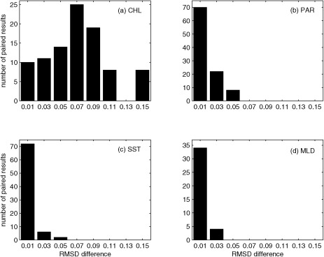
Difference in RMSD of logNPP_N=85 between paired results available for each participating model when only one of the input variables was from an alternate source: (a) chlorophyll (CHL) (24 models), (b) PAR (30 models), (c) SST (16 models), and (d) MLD (5 models).

4.2. Model Skill Assessment of NPP: Results Using Satellite Versus In Situ Chlorophyll (1998–2011, N=85)

Table 4 shows the RMSD between observations and model estimates in the 16 cases examined for all 32 participating models. Note that no statistical analysis was performed for Cases 9 to 16 in Models 13, 15, 17, 21–24, and 32, since these models required satellite products other than surface chlorophyll. Although RMSD varied between 0.56 and 0.88 among all cases, it was generally lower in the cases with in situ chlorophyll rather than satellite chlorophyll; however, a few models showed the opposite pattern (Models 12, 14, 16, 28, and 31). For example, Models 28 and 31 had higher RMSD values since those models had higher bias when using in situ chlorophyll (Table 5). However, Models 12 and 14 had lower bias and a higher correlation coefficient when using in situ chlorophyll (Case 9), but RMSD was still higher than when using satellite chlorophyll (Case 1). This is because a larger standard deviation in Case 9 increased uRMSD compared to Case 1. Model 16 shows the combined influence of the two factors just mentioned.

Table 5.

Mean (μ) and Standard Deviation (σ) of Estimated logNPP_N=85. RMSD, Bias, uRMSD, and Pearson's Correlation Coefficient (r) are Computed Between Each Model Estimate and In Situ logNPP_N=85 for Cases 1 and 9^a

Model	Case 1						Case 9
	μ	σ	RMSD	bias	uRMSD	r	μ	σ	RMSD	bias	uRMSD	r
1	2.79	0.21	0.64	0.30	0.57	0.46	2.71	0.36	0.56	0.22	0.52	0.58
2	2.86	0.23	0.68	0.37	0.56	0.46	2.78	0.40	0.59	0.29	0.51	0.58
3	2.73	0.29	0.60	0.24	0.55	0.49	2.56	0.56	0.56	0.07	0.55	0.58
4	2.82	0.29	0.65	0.34	0.56	0.47	2.69	0.49	0.56	0.21	0.52	0.59
5	2.88	0.15	0.70	0.40	0.58	0.48	2.81	0.21	0.63	0.32	0.54	0.58
6	2.43	0.32	0.57	−0.06	0.57	0.44	2.31	0.47	0.57	−0.18	0.55	0.54
7	2.83	0.21	0.66	0.35	0.57	0.46	2.69	0.40	0.56	0.21	0.52	0.57
8	2.82	0.28	0.66	0.33	0.56	0.45	2.69	0.41	0.56	0.20	0.52	0.57
9	2.68	0.22	0.64	0.20	0.60	0.30	2.64	0.37	0.58	0.15	0.56	0.48
10	2.67	0.22	0.65	0.18	0.63	0.19	2.55	0.33	0.59	0.06	0.58	0.40
11	2.71	0.30	0.68	0.22	0.65	0.19	2.71	0.42	0.62	0.22	0.58	0.44
12	2.58	0.27	0.56	0.09	0.55	0.49	2.42	0.67	0.61	−0.07	0.61	0.56
13	2.25	0.50	0.73	−0.23	0.69	0.28
14	2.69	0.28	0.59	0.20	0.55	0.49	2.48	0.74	0.65	−0.01	0.65	0.56
15	2.33	0.58	0.76	−0.16	0.75	0.24
16	2.40	0.27	0.56	−0.09	0.55	0.49	2.24	0.67	0.66	−0.25	0.61	0.56
17	2.07	0.50	0.80	−0.41	0.69	0.28
18	2.82	0.24	0.69	0.34	0.60	0.33	2.80	0.36	0.63	0.31	0.55	0.49
19	2.48	0.28	0.59	−0.01	0.59	0.36	2.36	0.47	0.56	−0.12	0.55	0.54
20	2.89	0.26	0.72	0.40	0.59	0.35	2.79	0.43	0.62	0.30	0.54	0.54
21	2.50	0.44	0.65	0.02	0.65	0.30
22	2.44	0.46	0.66	−0.04	0.66	0.30
23	2.73	0.31	0.65	0.24	0.60	0.35
24	2.69	0.31	0.63	0.21	0.60	0.36
25	2.77	0.25	0.65	0.28	0.58	0.39	2.62	0.45	0.56	0.13	0.55	0.54
26	2.61	0.33	0.60	0.12	0.59	0.39	2.50	0.56	0.57	0.01	0.57	0.54
27	2.54	0.32	0.57	0.05	0.57	0.44	2.41	0.54	0.56	−0.08	0.55	0.56
28	2.10	0.45	0.71	−0.39	0.60	0.43	1.92	0.75	0.87	−0.56	0.66	0.54
29	2.73	0.26	0.64	0.25	0.59	0.36	2.64	0.46	0.57	0.16	0.55	0.53
30	2.74	0.33	0.65	0.26	0.60	0.36	2.63	0.55	0.59	0.15	0.57	0.54
31	2.31	0.42	0.63	−0.17	0.61	0.39	2.16	0.73	0.74	−0.33	0.66	0.54
32	2.73	0.31	0.66	0.24	0.62	0.29
DR	2.61 ± 0.07	0.31 ± 0.03	0.65 ± 0.02	0.12 ± 0.07	0.59 ± 0.02	0.43 ± 0.02	2.58 ± 0.06	0.49 ± 0.05	0.59 ± 0.01	0.09 ± 0.06	0.55 ± 0.01	0.57 ± 0.004
DI	2.62 ± 0.06	0.30 ± 0.02	0.65 ± 0.01	0.13 ± 0.06	0.60 ± 0.006	0.34 ± 0.02	2.52 ± 0.07	0.49 ± 0.03	0.62 ± 0.02	0.03 ± 0.07	0.57 ± 0.01	0.51 ± 0.01
AB	2.62 ± 0.06	0.37 ± 0.03	0.65 ± 0.005	0.13 ± 0.05	0.63 ± 0.01	0.32 ± 0.01
All	2.61 ± 0.04	0.32 ± 0.02	0.65 ± 0.01	0.13 ± 0.04	0.60 ± 0.008	0.38 ± 0.02	2.55 ± 0.04	0.49 ± 0.03	0.61 ± 0.01	0.06 ± 0.04	0.57 ± 0.009	0.54 ± 0.009

^aIn each column, average model results (mean ± standard error) are also reported for three groups of participating models: depth‐resolved (DR) models (Models 1–8 and 12–17), depth‐integrated (DI) models (Models 9–11, 18–20, and 25–31), and absorption‐based (AB) models (Models 21–24, and 32). In Case 9, the gray shading indicates the models that have no values.

Based on the sensitivity test (Sect. 4.1), two of these 16 cases were selected for detailed analysis of model skill in reproducing NPP. These two cases used satellite PAR, reanalysis SST, and climatological MLD, but differed in their source of surface chlorophyll: one case used satellite chlorophyll (Case 1) and another case used in situ chlorophyll (Case 9). Figure 5 shows scatter plots of modeled NPP from both cases against in situ NPP values and Table 5 shows more in‐depth statistics of model results against in situ values including RMSD, bias, uRMSD, and correlation coefficients from these two cases. In general, models using in situ chlorophyll had lower RMSD, due to lower bias, and higher correlation coefficients (Table 5), and better represented the magnitude of the observed NPP variability (Figure 5). This is likely directly related to the fact that satellite chlorophyll substantially overestimated in situ chlorophyll at low chlorophyll concentrations and underestimated in situ chlorophyll at high chlorophyll concentrations (Figure 3b). In each case, whether using satellite or in situ chlorophyll, model performance was not significantly different between model types in terms of RMSD (Table 5), even when excluding a few models with the largest RMSD (e.g., Model 28). For satellite or in situ chlorophyll cases, most DR models, except Models 13, 15, and 17, performed better than DI models in terms of correlation coefficient.

Figure 5.

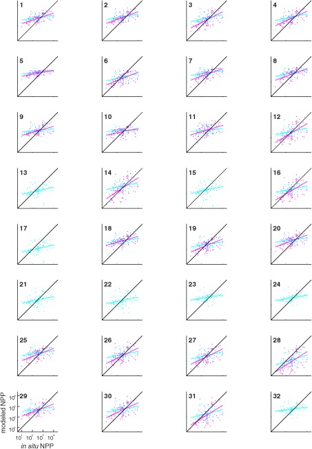
Scatter plots of modeled logNPP_N=85 using satellite chlorophyll (Case 1; blue) and in situ chlorophyll (Case 9; magenta) against in situ NPP (mgC m⁻² d⁻¹). The model number is indicated in the upper left and a black line indicates a 1:1 ratio.

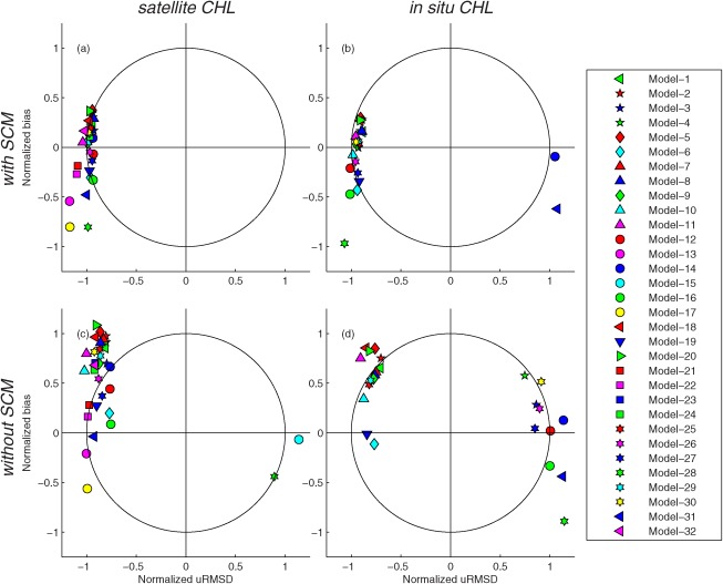
The skill statistics for all 32 models (Table 5) normalized by the standard deviation of in situ NPP are shown visually in the Target diagrams (Figure 6); the closer a model symbol is to origin, the better a model performs. The models generally produced lower RMSD (distance from origin) when using in situ chlorophyll (Figure 6b) compared to using satellite chlorophyll (Figure 6a) and thus more symbols appear inside the unit circle, i.e., ME>0, in Case 9. In terms of bias, roughly two‐thirds of the models overestimated the observed NPP, independent of which type of chlorophyll was used as input. When satellite chlorophyll was used as input, no model overestimated variability (all symbols were between −1.2 and −0.8 on the x axis), whereas when in situ chlorophyll was used, five of the models overestimated variability. Interestingly, the model results were clustered on either the positive or negative side of the x axis (uRMSD^*) with a magnitude between 0.8 and 1.2 in both cases, whereas the normalized bias largely varied between −0.6 and 0.6 along the y‐axis.

Figure 6.

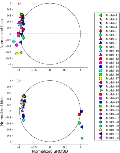
Target diagrams illustrating relative model performance in reproducing logNPP_N=85 using (a) satellite chlorophyll (Case 1) and (b) in situ chlorophyll (Case 9).

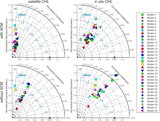
Taylor diagrams (Figure 7) were also used to visualize the relative skill of the models in terms of Pearson's correlation coefficient (r), normalized standard deviation, and normalized uRMSD without the information of bias. Note that a model performs better if it is closer to the reference point where r is 1.0, normalized uRMSD is 0, and the normalized standard deviation is 1.0. When satellite chlorophyll was used (Case 1), the models produced correlation coefficients that were mostly between 0.3 and 0.5 and the standard deviations of all the models were less than the standard deviation of the observed NPP (Figure 7a and see also Table 5). The models improved in estimating NPP when they incorporated in situ chlorophyll (Case 9) as evidenced by the higher correlation coefficients between the modeled and in situ NPP and the closer match between the standard deviations of the modeled and observed NPP than occurred for Case 1 (Figure 7b). While the Target diagrams, as described above, showed that the models were clustered in terms of normalized uRMSD (Figure 6), the clustering of the models in the Taylor diagrams was also due to a weak correlation and low variability of the model results as compared to in situ NPP. For example, assuming the model standard deviation is equal to the standard deviation of in situ NPP ( ${\sigma }_{model}/{\sigma }_{in\hspace{0.17em}situ}=1$), normalized uRMSD would be between 0.9 and 1.2 if r ranges between 0.3 and 0.6, respectively. In other words, as shown in the Taylor diagram (Figure 7), it is critical for models to have strong correlation (covariance) to lower uRMSD, even if model standard deviation is accurately represented.

Figure 7.

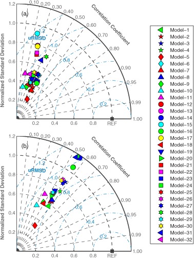
Taylor diagrams illustrating relative model performance in reproducing logNPP_N=85 using (a) satellite chlorophyll (Case 1) and (b) in situ chlorophyll (Case 9). The black square labeled as “REF” represents a perfect model, where the normalized standard deviation and the correlation coefficient are 1.0.

Boxplots were additionally used to characterize how well the modeled NPP reproduced the variability of the observed NPP (Figure 8). The distribution of the modeled NPP was generally symmetrical (i.e., a log‐normal distribution) and the median values were similar between the two cases for each model (Case 1 versus Case 9). However, when using satellite chlorophyll (Case 1), the models produced narrower boxes (interquartile ranges between the 25^th and 75^th percentiles) and shorter whiskers (Figure 8a) than when in situ chlorophyll concentrations were used (Case 9; Figure 8b). As a result, there were more outliers in Case 1 than in Case 9, indicating that the models in Case 1 using satellite chlorophyll overestimated NPP in low‐productivity regions/seasons and underestimated it in high‐productivity regions/seasons, relative to Case 9. Again, this is largely because satellite‐derived measurements overestimated chlorophyll at lower concentrations and underestimated it at higher concentrations (Figure 3b). Note that Models 13, 15, and 17 used Rrs to estimate surface chlorophyll from the Garver‐Siegel‐Maritorena semiempirical algorithm, which produced four outliers resulting in extremely low NPP (Figure 8a).

Figure 8.

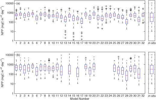
Boxplot of estimated logNPP_N=85 using (a) satellite chlorophyll (Case 1) and (b) in situ chlorophyll (Case 9). In situ NPP is shown on the right next to each plot. The box includes the middle 50% of NPP output (between 25th and 75th percentiles) and the central mark (red) is the median value of NPP. The whiskers extend to the most extreme (99% of data assumed to be normally distributed), not considering the outliers indicated as “+.”

Based on the skill assessment statistics described above (Table 5), models performing relatively better than others were selected for further analysis using the two following criteria: (1) bias was close to 0 (−0.1<bias<0.1) and (2) correlation coefficient was greater than the model average (r>0.38 for Case 1 and r>0.54 for Case 9). Four model results (Models 6, 12, 16, and 27) were selected for Case 1 and five model results (Models 3, 12, 14, 26, and 27) for Case 9. Using t‐test for equal mean, it was determined that the estimated NPP from the selected models was not statistically different from the in situ NPP_N=85 mean (not shown). From the cumulative distribution of logNPP_N=85 for these model results (Figure 9), it is again clear that the variability of NPP was underestimated using satellite chlorophyll (Case 1) although mean NPP was reproduced. Unlike Case 1, models using in situ chlorophyll (Case 9) successfully reproduced mean and variance in terms of magnitude distribution. Among the seven selected models, four (Models 3, 12, 14, and 16) required chlorophyll as well as satellite‐derived Rrs and two (Models 26 and 27) used empirically derived Z_{eu_derived} that was based on the relationship between in situ Z_eu and in situ surface chlorophyll using the AO data sets listed in Table 1 (log₁₀ Z_{eu_derived} = 0.0192 × log₁₀ in situ surface chlorophyll² ‐ 0.2303 × log₁₀ in situ surface chlorophyll + 1.4078). Models 12, 14, and 16 were also developed for the AO [Bélanger et al., 2013] and Models 14 and 16 were further tuned with Arctic‐relevant photosynthetic parameters [e.g., Huot et al., 2013].

Figure 9.

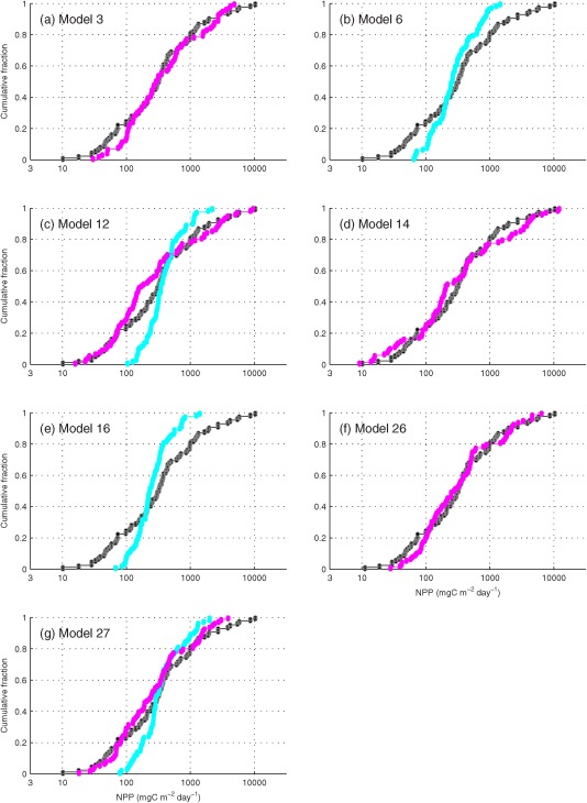
Cumulative distribution functions of logNPP_N=85 for the selected models, i.e., Models (a) 3, (b) 6, (c) 12, (d) 14, (e) 16, (f) 26, and (g) 27: blue=Case 1 NPP using satellite chlorophyll, red=Case 9 NPP using in situ chlorophyll, and black=in situ NPP.

4.3. Influence of the SCM in NPP Estimates (1998–2001, N=85)

When estimating NPP using ocean color models, one challenge is to take into account the impact of the SCM in optically complex waters like the AO. Hence a comparison of NPP model skill was made for times and locations when SCM were and were not present in the in situ NPP data set. For the stations with SCM, Figures 10a and 10b overall exhibit similar results to those in Figure 6; a few more models underestimated mean and/or variability of NPP as compared to when all data were used. In contrast, when SCM were not present, more models overestimated mean NPP with a greater magnitude as well as its variability (Figures 10c and 10d, respectively). Whether or not SCM were present, most models were clustered within the range of 0.7–1.0 in normalized uRMSD as shown earlier (Figure 6), but there was a large difference between cases in terms of correlation coefficient (Figure 11). Overall, the models had the highest correlation coefficient with in situ NPP when using in situ chlorophyll at the stations without SCM (Figure 11d) and the lowest when using satellite chlorophyll at the stations with SCM (Figure 11a).

Figure 10.

Target diagrams of (a) Case 1 using satellite chlorophyll (CHL) and (b) Case 9 using in situ CHL based on the stations where SCM existed (N=44), and (c) Case 1 and (d) Case 9 based on the stations where SCM was not present (N=39) among the 85 stations (1998–2011) in Figure 5. Note that two stations were excluded because no SCM information was available.

Figure 11.

Taylor diagrams of (a) Case 1 using satellite chlorophyll (CHL) and (c) Case 9 using in situ CHL based on the stations where SCM exists (N=44), and (b) Case 1 and (d) Case 9 based on the stations where SCM was not present (N=39) among the 85 stations (1998–2011) in Figure 6. Note that two stations were excluded because no SCM information was available.

4.4. Vertical Profiles of NPP in DR Models (1998–2011, N=85)

Vertical profiles of NPP estimated by the 11 DR models (Models 1–8, 12, 14, and 16) were also compared to in situ vertical profiles at the 85 sampling stations (1998–2011). Because sampling depths were different at each station, in situ NPP as well as the model results were grouped into ten layers: 0–2 m, 2–5 m, 5–10 m, 10–15 m, 15–20 m, 20–30 m, 30–40 m, 40–50 m, 50–60 m, and 60–100 m. The participants provided NPP profiles only for Case 1 (satellite chlorophyll and PAR, reanalysis SST, and climatological MLD) and Case 16 (in situ chlorophyll, reanalysis PAR, in situ SST, and in situ MLD) including model Z_eu estimates. Note that only DR models were asked to provide vertical profiles for Case 1 and 16, and Models 13, 15, and 17 were excluded because they had no results for Case 16. The DR models generally overestimated NPP (mean and variability) and Z_eu in both cases (Figure 12a). In July, mean in situ and modeled NPP were both highest just below the surface (2–5 m). In contrast, variability of in situ NPP was high down to 40 m, whereas variability of modeled NPP was only high in the uppermost 10 m (Figure 12b). This high observed variability at depths below 20 m was not captured in the DR models. Unlike in July, in August mean and variability of in situ NPP were both highest at the surface layer (0–2 m and 2–10 m, respectively) and decreased quickly. This trend was reproduced in the models; however, the in situ NPP was very low below 20 m depth, whereas the models overestimated NPP down to 50 m depth (Figure 12c).

Figure 12.

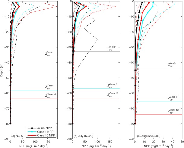
Vertical profiles of the mean in situ (black) NPP and the mean NPP of the 11 depth‐resolved models (Models 1–8, 12, 14, and 16) in (a) all months (N=85), (b) July (N=29), and (c) August (N=38): Case 1 NPP (blue) and Case 16 NPP (red) with the averaged confidence interval of 1 standard deviation (dotted lines). NPP was grouped and averaged at given depth layers: 0–2 m, 2–5 m, 5–10 m, 10–15 m, 15–20 m, 20–30 m, 30–40 m, 40–50 m, 50–60 m, and 60–100 m. The average in situ and model Z_eu (Case 1 and 16) are also shown.

The model skills of the 11 DR models at different depth layers in Cases 1 and 16 were assessed using the Target and Taylor diagrams (Figure 13). All models overestimated NPP except one model (Model 6), which had very low NPP below 10m (seven symbols with negative normalized bias less than −0.25 in Figures 13a and 13b). Almost all models underestimated the variability, except in the surface layer of 0–10 m in Case 16 using in situ chlorophyll (Figure 13b). The models also showed the highest correlation with in situ NPP in this surface layer (Figure 13d), but this was not so for Case 1 using satellite chlorophyll (Figure 13c). In general, the DR models performed very poorly at the middepth layer (15 ‐ 40 m), where variability of in situ NPP was greater than estimated NPP (e.g., Figure 12b), because uRMSD was high and correlation coefficient was low.

Figure 13.

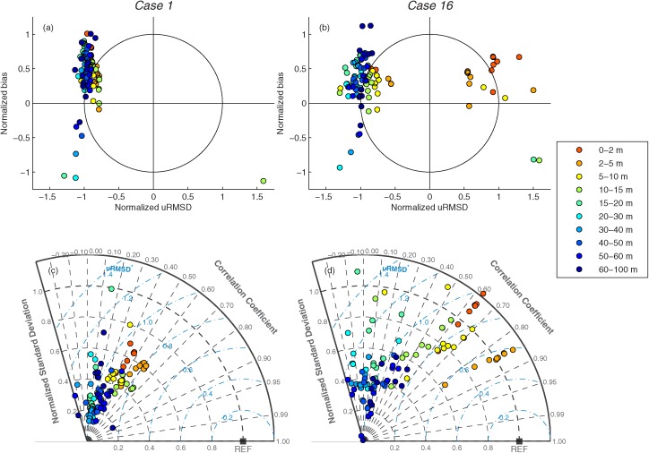
(a, b) Target and (c, d) Taylor diagrams of (left) Case 1 and (right) Case 16, representing relative model performance in reproducing logNPP_N=85 by the 11 depth‐resolved models (Models 1–8, 12, 14 and 16) using satellite and in situ chlorophyll, respectively. The symbols indicate the statistics between in situ and estimated NPP at various depth layers: 0–2 m, 2–5 m, 5–10 m, 10–15 m, 15–20 m, 20–30 m, 30–40 m, 40–50 m, 50–60 m, and 60–100 m.

4.5. Regional and Seasonal NPP (1988–2011, N=455)

In order to utilize the entire in situ data set, Case 16 was selected from 1988 to 2011 for the next two exercises, using 16 models out of the 32 participating models, after excluding those requiring satellite‐derived products (Models 3, 12–17, 21–24, and 32) and/or producing NPP at less than 455 stations in total (Models 5, 6, 10 and 11). The 16 remaining models estimated NPP using in situ chlorophyll, NOAA/NCEP reanalysis daily PAR, in situ SST, and in situ MLD (Figure 3). We examined the performance of model skill in four different time periods that have a similar number of stations (April–June, July, August, and September–November), in two different regions (bottom depth ≤200 m and >200 m), and under two different sea ice conditions (< and ≥ 15% ice concentration) using the Target and Taylor diagrams.

Overall, the selected models performed better in fall (September–November) or at deep‐water stations (depth > 200 m) in terms of uRMSD (Figures 14a and 14b) as well as correlation coefficients (Figures 14c and 14d), when and where NPP was relatively low, respectively (Table 2). In addition, the models reproduced NPP relatively well (lower RMSD and higher correlation coefficient) in sea ice‐covered regions compared to sea ice‐free regions (Figures 14b and 14d) even though the distribution of in situ NPP values was similar between the two regions (Table 2). On the other hand, the models performed poorly in July–August and at shallow‐water stations (depth < 200 m), when and where NPP was relatively high, respectively (Table 2). Although RMSD varied spatially and temporally, the model performance in a given month (bloom or postbloom) and region (depth or ice coverage) was mostly determined by bias rather than uRMSD and/or correlation coefficient.

Figure 14.

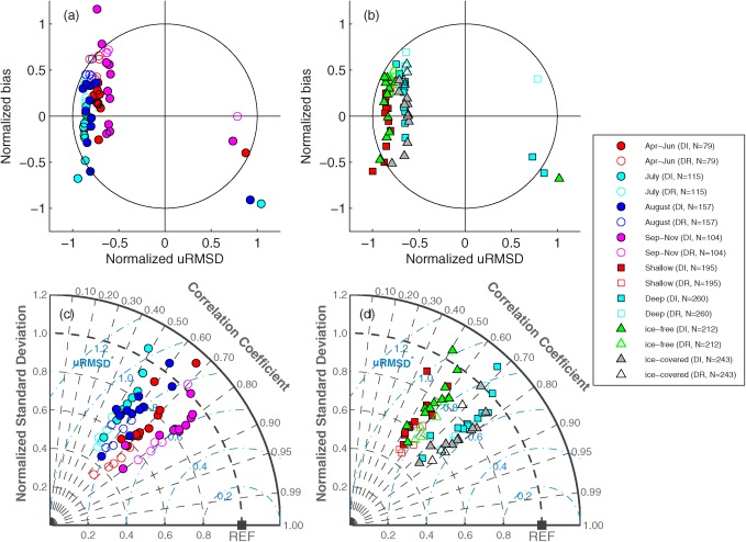
(a, b) Target and (c, d) Taylor diagrams of Case 16 (N=455) using in situ chlorophyll (1988–2011), illustrating relative model performance in reproducing logNPP over different (left) months and (right) regions. The symbols indicate the statistics between in situ and estimated logNPP in four different periods (April–June, July, August, and September–November), two different regions (shallow‐water stations where water depth is less than 200 m and deep stations where water depth is greater than 200 m), two different sea ice conditions (ice‐free stations where sea ice concentration was less than 15% and ice‐covered stations where sea ice concentration was greater than 15%), and two different model types (5 depth‐resolved (DR) and 11 depth‐integrated (DI) models). See text for further details.

In a final component of this analysis, in situ and modeled daily NPP were projected onto a 100 km EASE‐Grid map to illustrate the spatial pattern of NPP in the AO (Figure 15a). In situ NPP was relatively higher in the Chukchi Sea, the Canadian Archipelago, and the Nordic Seas and lower in the Beaufort Sea and the central Arctic Basin. Based on the average results from Case 16 (N=455), the simulated NPP was compared regionally with in situ data. In general, the models have a strong tendency to overestimate NPP in lower productivity regions and underestimate NPP in higher productivity regions. In situ and modeled NPP were highly correlated in the central Arctic Basin (r=0.82, p<0.01; Figure 15e) where most of the in situ NPP were measured at deep‐water, sea ice‐covered stations and weakly correlated in the Chukchi Sea (r=0.57, p<0.01; Figure 15d) where most of the in situ NPP were measured at shallow‐water, sea ice‐free stations.

Figure 15.

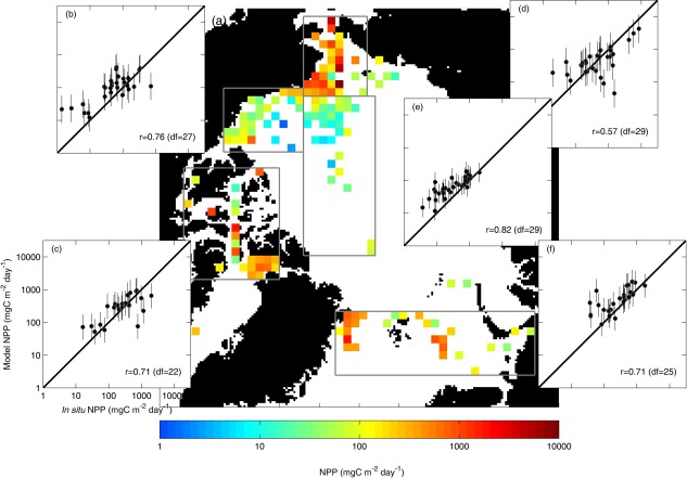
(a) In situ NPP projected on the EASE‐Grid map, and average estimation with an error bar (± 1 standard deviation from the mean) from 16 NPP models (N=455) was regionally compared to in situ values in (b) Beaufort Sea, (c) Canadian Archipelago, (d) Chukchi Sea, (e) central Arctic Basin, and (f) Nordic Seas; all inserts have the same axis units as in Figure 15c. A solid‐line is a slope of 1.0 and the correlation coefficient (r) with degrees of freedom (df=number of grid cells‐2) is shown in the lower right of each insert.

5. Discussion

Our main objective was to determine sources of uncertainty in the performance of various NPP models based on satellite ocean color and chlorophyll measurement. A large number of models (N=32) participated in this PPARR exercise and individual model skill was assessed primarily by computing mean, variance, and RMSD (bias and uRMSD) as well as other statistical tools to determine how well each model reproduced NPP in the AO. Compared to previous PPARR exercises [Campbell et al., 2002 ; Friedrichs et al., 2009 ; Saba et al., 2010, 2011], in situ integrated NPP in the AO exhibited the widest variability of data: more than 4 orders of magnitude between minimum and maximum NPP (1 to 10,000 mgC m⁻² d⁻¹). Model skills presented in previous PPARR studies varied substantially from one region to another; RMSD ranged mostly between 0.1 and 0.5 from tropical waters to high latitudes. In contrast, this study showed that RMSD in the AO varied from 0.56 to 0.80 (see Table 4) which was much greater than RMSD in any other region so far studied, indicating the lowest model skill (the highest RMSD) for this polar region. Carr et al. [2006] showed that NPP model estimates had the widest range of values for the AO at basin scale, when using monthly, satellite‐derived data only. Saba et al. [2011] found that the highest model skill was observed in the deep‐water regions with low NPP variability; however, the AO was not included in that study. In contrast, model skill was lowest in the shallow‐water regions where NPP variability was highest, such as in coastal areas of the Mediterranean Sea [Saba et al., 2011]. In this AO study, the model‐data misfit mainly stemmed from an underestimation of NPP variability by the models, because of a large variability of the in situ data––especially in shallow‐water regions like the Chukchi Sea (i.e., Figure 15d)––that the models were unable to reproduce.

It should be remembered that the cumulative maximum error of NPP propagated from field measurement precision to algorithm precision has been shown to account for 39% of RMSD in the case of a classical empirical model also dependent on chlorophyll only [Eppley et al., 1985] and has been estimated as 72% [Saba et al., 2011] to ± 100% [Balch et al., 1992; Campbell et al., 2002] in more complex models. These estimates include the uncertainties associated with the determination of in situ chlorophyll (6–21%) [Lorenzen and Jeffrey, 1980] (e.g., fluorometric versus HPLC data) and with satellite chlorophyll (median absolute percent difference of 33% [Bailey and Werdell, 2006]; RMSD of 0.29 log unit [Moore et al., 2009]; and satellite pigment accuracy per se of ±0.17 log unit [O'Reilly et al., 1998]). It should be noted that previous model intercomparisons dealt with integrated NPP estimates that respond differently to environmental perturbations than surface primary production [Balch et al., 1992; Saba et al., 2010]. Finally, it has become clear that not all NPP is necessarily contained within the algal cells in the particulate fraction (as represented by most of the in situ data herein) but that a significant fraction (sometimes as much as 50%) is quickly released by the algal cells as dissolved primary production in Arctic waters [Gosselin et al., 1997; Klein et al., 2002; Vernet et al., 1998], causing an underestimation of NPP.

A primary result of this model inter‐comparison effort highlights that most ocean color NPP models using surface chlorophyll performed better in the AO when in situ measurements rather than satellite‐derived properties were used; the skill of certain models decreased dramatically if satellite chlorophyll was used instead. This is because satellite chlorophyll was underestimated at higher concentration and overestimated at lower concentrations compared to in situ values in the AO (see Figure 3b) [also Cota et al., 2004; Matrai et al., 2013]. As a result, modeled NPP variances were substantially underestimated (Figure 8a), resulting in relatively weaker correlation between in situ and estimated NPP (Figure 7a). The use of semianalytical algorithms to estimate surface chlorophyll, such as the Garver‐Siegel‐Maritorena model, did not improve the results (Models 13, 15 and 17 versus Models 12, 14, and 16). Hence, an accurate retrieval or measurement of surface phytoplankton chlorophyll becomes critical to estimate NPP in the AO using OCMs [i.e., Balch et al., 1992; Saba et al., 2010]. Uncertainties in estimating NPP from remotely sensed ocean color have been largely attributed to surface chlorophyll [Friedrichs et al., 2009; Saba et al., 2010, 2011] and photosynthetic parameters [Milutinović and Bertino, 2011] relative to other input variables. In our case, we showed that the models that utilized MLD in estimating NPP were least sensitive to the type of MLD data (in situ versus climatology), possibly because of a shallow mixed layer in the AO [Peralta‐Ferriz and Woodgate, 2015], suggesting that the spatio‐temporal variability of MLD was relatively weak in our AO data sets (Figure 3e).

The low irradiance and low water temperature prevailing in polar seas are associated with unique bio‐optical and photosynthetic parameters reflecting these extreme environments that must be accounted for in primary production models [e.g., Rey, 1991; Arrigo et al., 2008]. The interactions between these factors have resulted in overestimates of low NPP and underestimates of high NPP by remote sensing (Figure 5). Many of the models also incorporated PAR and SST in this study, but there was little difference in the overall performance of the models. This is because the two different sources for each input variable exhibited a similar distribution (Figures 3c and 3d), indicating that the AO is well represented in reanalysis data of PAR and SST. The range of PAR in the AO is comparable to that in previous PPARR exercises in tropical to temperate regions [e.g., Campbell et al., 2002; Friedrichs et al., 2009; Saba et al., 2011]; however, SST was generally low and narrowly ranged, only between −2 and 6°C, in the AO (Figure 3d). Sixteen NPP algorithms include temperature‐dependent functions which are used to correct temperate water values adopted for phytoplankton physiological parameters (i.e., the maximum photosynthetic rate normalized to chlorophyll, ${\mathrm{P}}_{\text{max}}^{\mathrm{B}}$ or similar parameters). For instance, the correction from a 20°C rate to the value for a temperature of 0°C means a reduction by about 70% in the maximum photosynthetic rate [e.g., Eppley, 1972]. However, the effect of temperature on ${\mathrm{P}}_{\text{max}}^{\mathrm{B}}$ was not significant over the temperature range observed in the southern Beaufort Sea during the MALINA cruise [Huot et al., 2013]. Although the various models performed poorly in reproducing the in situ NPP values in the AO, the models were less sensitive to uncertainties in SST, suggesting that temperature dependence in NPP algorithms may be sufficient in the AO or that the influence of temperature on phytoplankton physiology, within the narrow range of observed SST, may be insignificant compared to surface irradiance.

Although it still is a subject of much discussion, errors from model‐derived NPP omitting SCM vary significantly temporally and spatially from one study and one region to another [Ardyna et al., 2013; Brown et al., 2015; Cherkasheva et al. 2013; Arrigo et al., 2011; Hill et al., 2013; Martin et al., 2013; Zhai et al., 2012]. Since most OCMs rely on surface chlorophyll and do not account for the presence of SCM in their algorithms during postbloom season (July–September), one can expect that the presence of a SCM may bias their estimates of NPP [e.g., Martin et al. 2010]. Contrary to the SCM observed at lower latitudes [Cullen, 1992], the Arctic SCM often corresponds to a maximum in particulate carbon and primary production [Martin et al., 2010]. However, the highest NPP levels were found in the upper 20 m in the Chukchi Sea whereas the depth of SCM was observed mostly below 15 m [Coupel et al., 2015; Brown et al., 2015], indicating that high chlorophyll does not always account for high NPP in this polar water column. Figure 12 shows that mean in situ NPP in the AO was highest at the surface (0–10 m) but its variability was highest between 20 and 30 m in the lower euphotic zone where SCM usually occur, especially in July (Figure 12b). However, this pattern was not clearly exhibited in August, when mean and variability of in situ NPP peaked at the surface (0–10 m) and declined with depth (Figure 12c). When in situ NPP was averaged temporally and spatially, the maximum of subsurface NPP variability was significantly dampened at pan‐Arctic and/or annual scales (Figure 12a).

When our analyses were expanded to include more in situ data from 1988 to 2011 (N=455; Figures 14 and 15), thus using a decade of data prior to the advent of remote sensing, the models performed poorly in July (Figures 14a and 14c), when the mean and variance of in situ NPP were high (Table 2). This is likely because the models could not capture the presence of the July SCM [e.g., Arrigo et al., 2011; Ardyna et al., 2013], resulting in high uRMSD and low correlation. The models were also regionally compared to in situ NPP again showing that the models overestimated NPP in low productivity regions (the Beaufort Sea and the central Arctic Basin) and underestimated it in high productivity regions (the Chukchi Sea). That the models performed worst in a highly productive region such as the Chukchi Sea may suggest that the underestimation of NPP is possibly linked to the existence of a SCM which Brown et al. [2015] describe to be deeper than the NPP maximum and the MLD historically, especially in July and the rest of the summer. Or, the model performance could be due to the fact that the majority of the models were originally developed for regions other than these optically complex polar waters, rather mostly for Case‐1 waters, for which light penetration differs substantially than in the AO [Antoine et al., 2013].

When a SCM is present, AO ocean color‐based NPP is expected to be underestimated, as a result of the omission of phytoplankton chlorophyll now at the SCM [e.g., Hill et al., 2013 , Zhai et al., 2012]. In this study, we confirmed this expectation, highlighting the failure of the models to capture the NPP variability at the stations where a SCM was present, especially when using satellite chlorophyll as input data. In contrast, the models performed better at the stations without SCM, particularly in terms of correlation; albeit that NPP was overestimated. Nonetheless, some models performed well on a pan‐Arctic scale in terms of bias (Table 5 and Figure 6). This suggests that the overestimated NPP in the absence of SCM could be compensated by underestimation of NPP due to omission of the SCM [Arrigo et al., 2011; IOCCG, 2015], or that vertical variations in chlorophyll have a limited impact on annual, depth‐integrated NPP [Ardyna et al., 2013]. Although the SCM is a ubiquitous feature throughout the Arctic Ocean on a seasonal basis, processes involved in developing/maintaining SCM are possibly different from coastal to offshore regions [Bergeron and Tremblay, 2014; McLaughlin and Carmack, 2010]. Hence, the effect of the SCM could be most important on a regional scale and more pronounced in mid‐summer, and may correspond to high NPP at middepths in highly stratified oligotrophic waters, such as the Beaufort Sea [Weston et al., 2005 ; Martin et al., 2010, 2013; Tremblay et al., 2008], while the SCM accounts only for a low fraction of integrated NPP on an annual basis over the pan‐Arctic domain [Arrigo et al., 2011; IOCCG, 2015]. However, the location of the SCM can be critical to understanding higher trophic levels and pelagic‐benthic coupling [Wassmann and Reigstad, 2011].

Of all the participating models, sea ice information was only taken into account in Model 31 [Fernández‐Méndez et al., 2015], which was specifically developed for the ice‐covered region (north of 75°N) where satellites cannot measure most ocean properties. This may pose a limitation when applying these models to the entire AO, especially in areas where subice and/or ice‐algal blooms are dominant. It should be noted that the models were provided with incoming PAR, computed above the sea ice surface, which likely exceeded the subice light levels available for the in situ primary production incubations provided as field data. Nonetheless, it is surprising that, whether sea ice‐covered or not, in situ NPP values were more or less similarly distributed in the two regions (Table 2), supporting significant phytoplankton production under the sea ice cover [Gosselin et al., 1997; Pomeroy, 1997]. The models generally performed better in ice‐covered regions than in ice‐free regions, especially in terms of correlation coefficient (Figure 14d) and they even performed better in the stations with higher sea ice concentration (not shown). In other words, the models did a relatively poor job of capturing NPP variability in physically dynamic, ice‐free regions where fronts, upwelling, and other mesoscale physical features may occur. Model 31 also produced NPP in sea ice‐free areas where it is not expected to give good results, and it performed better with satellite chlorophyll than with in situ chlorophyll in terms of RMSD, though it significantly underestimated the mean NPP when using in situ chlorophyll.

Our results show that ocean color NPP models for the AO were challenged by the strong spatio‐temporal variability of the in situ data. Such variability is controlled by discontinuous data availability as well as by processes that interfere with remote sensing of ocean chlorophyll, such as subpixel ice contamination [Bélanger et al., 2007]. Other obstacles also exist in the AO that pertain to the remote sensing of ocean color and the derivation of accurate estimates of surface chlorophyll needed for the simulation of NPP [Babin et al., 2015]. These range from those on cellular scales, i.e., an enhanced pigment packaging effect common in polar waters [e.g., Brunelle et al., 2012; Matsuoka et al., 2011], to those on regional scales, i.e., signal interference by land‐derived, river‐borne colored dissolved organic matter (CDOM) [e.g., Brunelle et al., 2012 ; Matsuoka et al., 2007, 2011, 2013; Rachold et al., 2004], and basin scales, i.e., signal loss by sea ice and cloud cover [IOCCG, 2015]. Recent bio‐optical analyses in the western Arctic indicate a positive bias resulting from currently used chlorophyll algorithms and their treatment of CDOM [Chaves et al., 2015], rather than from the radiometric reflectance data per se collected by the satellite‐borne sensor. Previous studies, on the other hand, found nonuniform biases in estimating chlorophyll on a pan‐Arctic basis, but with consistent patterns of underestimation of surface chlorophyll in the Labrador Sea [Cota et al., 2003] and overestimation in the Beaufort, Chukchi and Nordic Seas [Ben Mustapha et al., 2012; Matsuoka et al., 2007; Stramska et al., 2003; Wang and Cota, 2003]. In this study, the absorption‐based models that included a way to reduce the impact of Arctic CDOM, pigment packaging, and nonalgal matter in their algorithms (Models 21 and 22) exhibited both lower bias and higher standard deviation close to in situ NPP (Table 5 and Figure 6a) when using remotely sensed data. The algorithm for Models 12, 14, and 16 was originally developed for the AO [Bélanger et al., 2013]; Models 14 and 16 further incorporated photosynthetic parameters derived from Arctic data sets [Huot et al., 2013]. Models 26 and 27 modified their original algorithms by including empirically derived Z_eu information and photosynthetic parameters based on the Arctic data. The models specifically tuned for the Arctic environment (Models 12, 14, 26, and 27) outperformed other ocean color models in terms of mean, variance, and correlation, especially when using in situ chlorophyll. However, although photosynthetic parameters were also tuned for the AO, modeled NPP was still significantly underestimated and weakly correlated in Models 13, 15, and 17 using Rrs‐derived chlorophyll based on the Garver‐Siegel‐Maritorena semianalytical algorithm. Clearly, an improved, regional chlorophyll algorithm tuned for the AO will result in more accurate NPP [Bélanger et al., 2007], even though previous attempts [Cota et al., 2004; Wang and Cota, 2003] have had mixed successes [Ben Mustapha et al., 2012; Matsuoka et al., 2007].

Although skill varied substantially among the participating models, most models significantly underestimated the variability of NPP, often by more than a factor of two, regardless of model type or complexity. On the positive side, some models presented almost no bias. Thus, the models with a greater skill were generally those that exhibited the least bias and that best simulated integrated NPP variability, though the latter varied relatively little among, and was similarly underestimated by, most of the participating models. The specific models that demonstrated the greatest skill varied depending on which skill metric was used. For example, if the correlation coefficient was used as a single skill metric, some models performed relatively well compared to others, but their bias was large (e.g., Models 5 and 28), resulting in relatively higher RMSD values. Similarly, in terms of reproducing the observed mean NPP, especially when using satellite chlorophyll (Case 1), Models 21 and 22 had one of the lowest bias, but these models were very weakly correlated with the in situ NPP, resulting in relatively higher RMSD values (Table 5 and Figure 5). Furthermore, one should be cautious that lower bias and higher correlations often yield higher RMSD when the standard deviation of model results is greater than that of the in situ data, e.g., Model 14 in Case 9. Therefore, it is critical to use multiple skill metrics, since correlation can be substantially different even if RMSD are similar or vice versa. When using in situ chlorophyll (Case 9), there were five models (Models 3, 12, 14, 26, and 27 in Figure 9) that reproduced the NPP distribution (equal mean and variance based on the null hypothesis using t‐test and F‐test, respectively; not shown) but did not necessarily show a one‐to‐one relationship with a slope of 1.0 (Figure 5), suggesting that the models failed to capture small‐scale variability, extreme events, or, perhaps, the SCM.

It is clearly a challenge for OCMs to be applied in Case‐2 waters which are optically complex and often productive at the same time, such as in the AO in summer. Furthermore, the widespread presence of CDOM from Arctic rivers significantly changes the optical properties in AO waters [Anderson and Amon, 2014; Antoine et al., 2013]. Our study strongly recommends that the current algorithm used to remotely derive chlorophyll should be improved for the AO [Antoine et al., 2013; Lee et al., 2015; Chaves et al., 2015]. This PPARR exercise suggests that bio‐optical parameters (e.g., quantum yield, absorption coefficients, and photosynthetic rates) in ocean color models need to be tuned for the AO, such that the development of regional‐ and/or seasonal‐specific models can lead to improved estimates of NPP for a better understanding of current and future trends of NPP. In addition, in order to examine seasonal and regional characteristics of primary productivity in the AO, it is desirable to have extensive field measurements with international collaborations covering various areas in the AO. Because the current in situ data sets are also skewed temporally and spatially, the results from their analysis may be biased toward the western Arctic during summer months. Although the estimated NPP range may be of similar magnitude for the pan‐Arctic Ocean, the processes involved and their relative importance are very different in the various areas of the AO [Carmack and Wassmann, 2006; Wassmann, 2011].

Appendix A. Model Descriptions

A1. Model 1

This is a model based on Morel [1991], which is formulated using chlorophyll specific wavelength‐resolved absorption and quantum yield. Temperature dependence is given by the parameterization of the maximum photosynthetic yield ( ${\mathrm{P}}_{\text{max}}^{\mathrm{B}}$), which follows Eppley [1972]. The chlorophyll profile is determined to be well‐mixed or stratified according to the ratio of MLD and the euphotic depth, and if stratified, assigned a Gaussian profile as in Morel and Berthon [1989]. Mean photo‐physiological parameters are from Morel et al. [1996]. The model is run in its “satellite” version [Antoine et al., 1996], where NPP is the product of integral biomass, the daily irradiance, and ψ*(the cross section of algae for photosynthesis per unit of areal chlorophyll biomass).

A2. Model 2–4

These models [Mélin, 2003; Mélin and Hoepffner, 2011] follow that of Platt and Sathyendranath [1988] as implemented at global scale by Longhurst et al. [1995]. It uses biogeographical provinces to define the values of the parameters to describe the light‐photosynthesis curve and the chlorophyll depth profile. Photosynthetic parameters were updated using an extended data set provided by the Bedford Institute of Oceanography and an extensive literature review. Spectral surface irradiance is first estimated independently with the model of Gregg and Carder [1990] combined with a correction for cloud cover and then scaled to match the PAR values provided for the exercise. Spectral light is subsequently propagated in the water column with a Case‐1 bio‐optical model with updated parameterizations of the inherent optical properties. All changes to the original implementation of Longhurst et al. [1995] are detailed by Mélin [2003]. With respect to the standard configuration (Model 4), two other versions were tested. Model 2 adopted the parameterization of Ardyna et al. [2013] to define the vertical shape of the chlorophyll profile. Model 3 used satellite‐derived reflectance values and the QAA [Lee et al., 2002] to compute an independent estimate of the absorption by chromophoric dissolved organic matter that substitutes the contribution foreseen by the Case‐1 water model in the standard model.

A3. Model 5 and 6

These models derived spectral irradiance using Tanré et al. [1990] scaled to the PAR values provided in the exercise, and applies a wavelength dependent absorption as a function of chlorophyll as spectral irradiance is propagated through the water column. Quantum yield varies with depth and is parameterized as a maximum value times both a light‐dependent term [Bidigare et al., 1992; Waters et al., 1994] and a temperature dependent term. Temperature dependence was assumed to be sigmoidal, and was based on a vertical profile of temperature derived from SST and MLD. For Model 5, the chlorophyll profile was assumed constant and equal to the surface chlorophyll. For Model 6, the chlorophyll profile was assumed constant to the MLD, followed by a small chlorophyll max and then a decrease to 20% of the surface chlorophyll. The chlorophyll maximum was 0.1 mg m⁻³ larger than the surface chlorophyll. Parameterizations were primarily derived from temperate and tropical areas. While CDOM absorption can be incorporated in the model, it was not provided in the exercise.

A4. Model 7

This model is an implementation of the Morel [1991] model in which the depth distribution of chlorophyll is assumed constant throughout the water column. The broadband incident PAR is spectrally resolved using a look‐up‐table generated from a single run of the Gregg and Carder [1990] marine irradiance model where the effects of clouds and aerosols are essentially linearly scaled. The model uses 60 min time and 10 m depth steps at 5 nm wavelength resolution when run using the global data sets [Smyth et al., 2005].

A5. Model 8

In this model, the depth distribution of PAR is given by an empirical equation of light attenuation, which is determined by the surface chlorophyll. The vertical distribution of chlorophyll is determined empirically with the vertical distribution of PAR and surface chlorophyll. The products between the chlorophyll and the carbon fixation rate, which is defined as a function of PAR and temperature, are integrated for the day time and for the euphotic depth to give the total productivity [Asanuma, 2006].

A6. Model 9

This model uses an artificial neural network to perform a generalized nonlinear regression of NPP on several predictive variables, including latitude, longitude, day length, MLD, SST, a maximum carbon fixation rate within a water column ( ${\mathrm{P}}_{\text{opt}}^{\mathrm{B}}$) computed according to Behrenfeld and Falkowski [1997a], PAR, and chlorophyll [Scardi, 2000; Scardi, 2001].

A7. Model 10–11

These models use support vector machine (SVM) as the nonlinear transfer function between ocean primary productivity and chlorophyll‐a concentration, euphotic layer depth, PAR, maximum carbon fixation rate, and day length [Tang et al., 2008]. In Model 10, the maximum carbon fixation was estimated by using a seventh‐order polynomial function of SST [Behrenfeld and Falkowski, 1997a]. The euphotic layer depth was estimated using the integrated chlorophyll [Morel and Berthon, 1989]. Model 11 is similar to Model 10 except that the maximum carbon fixation rate was estimated as a SVM‐based nonlinear function of SST, chlorophyll, and PAR.

A8. Model 12–17

All models assume vertically homogeneous chlorophyll profiles and use Rrs to estimate spectral diffuse attenuation coefficient of downward irradiance (K_d) applying the QAA [Lee et al., 2002, 2005]. Model 12 and 13 based on ${\mathrm{P}}_{\text{max}}^{\mathrm{B}}$ as Bélanger et al. [2013] use measured chlorophyll and Rrs‐derived chlorophyll, based on the Garver‐Siegel‐Maritorena semiempirical algorithm, respectively. Model 14 and 15 use measured chlorophyll and Rrs‐derived chlorophyll, respectively, but ${\mathrm{P}}_{\text{max}}^{\mathrm{B}}$ is based on Huot et al. [2013]. If chlorophyll is less than 0.1 mg m⁻³, Model 14 and 15 use equation (2) in Huot et al. [2013]. Otherwise, Model 14 and 15 uses equation (3) in Huot et al. [2013]. Model 16 and 17, based on ${\mathrm{P}}_{\text{max}}^{\mathrm{B}}$ from equation (4) in Huot et al. [2013], use measured chlorophyll and Rrs‐derived chlorophyll, respectively.

A9. Model 18

This vertically generalized production model (VGPM) variant formulates ${\mathrm{P}}_{\text{opt}}^{\mathrm{B}}$ as a function of SST and chlorophyll [Kameda and Ishizaka, 2005; Yamada et al., 2005]. The model is based on the assumption that phytoplankton consists of large and small phytoplankton groups, which have specific chlorophyll productivities and temperature functions such that changes in chlorophyll concentration depends on the abundance of large phytoplankton.

A10. Model 19

This model is identical to the original version of the VGPM model developed by Behrenfeld and Falkowski [1997a]. The implementation for this model closely matches the code found on the Oregon State University primary productivity website (see http://www.science.oregonstate.edu/ocean.productivity/vgpm.code.php). For ${\mathrm{P}}_{\text{opt}}^{\mathrm{B}}$, a Horn formulation (recursive) of the original 7th order polynomial of temperature was used for better numerical stability. The calculation for NPP was formulated for integration to 1% euphotic depth and there were no checks for euphotic depth exceeding actual depth. As with the original model, there was also no treatment of MLD.

A11. Model 20

This model is the original default version of VGPM developed by Behrenfeld and Falkowski [1997a].

A12. Model 21–24

All models are based on the VGPM [Behrenfeld and Falkowski, 1997a] and assume homogeneous chlorophyll profile. ${\mathrm{P}}_{\text{opt}}^{\mathrm{B}}$×C_surf in the VGPM was replaced by an empirical function of absorption coefficient of phytoplankton at the sea surface (a _ph (0−)) for Models 21 and 22 [Hirawake et al., 2012], or by absorbed radiation by phytoplankton (a _ph(0−) × PAR/day‐length) for Models 23 and 24 (SGLI/GCOM‐C, TBD). Models 21 and 23 used spectrally averaged absorption coefficient, ā _ph(0−), and Models 22 and 24 used absorption coefficient at 443 nm, a _ph(443, 0−).

A13. Model 25

This model is based on equation (4) presented in Balch et al. [1992]. ${\mathrm{P}}_{\text{max}}^{\mathrm{B}}$ is a median value (1.14 mgC mgChl⁻¹ h⁻¹) based on previously published measurements in the AO [Platt et al., 1982; Smith et al., 1985; Harrison and Platt, 1986; Platt et al., 1987; Rey, 1991; Harrison and Cota, 1991; Sakshaug and Slagstad, 1991; Stockwell et al., 2001; Tremblay et al., 2006; Yamaguchi et al., 1996]. The attenuation coefficient for PAR was formulated from Nelson and Smith [1991].

A14. Model 26

This model is a variant of Eppley‐VGPM [Eppley, 1972; Antoine and Morel, 1996; Behrenfeld and Falkowski, 1997a] using Z_eu empirically derived for the AO (see the section 4.2).

A15. Model 27

This is a variant of the algorithm by Howard and Yoder [1997], which integrates NPP to Z_eu empirically derived for the AO (see the section 4.2) rather than to MLD. ${\mathrm{P}}_{\text{max}}^{\mathrm{B}}$ and the initial slope of the photosynthesis (α) are median values (1.14 mgC mgChl⁻¹ h⁻¹ and 0.06 mgC mgChl⁻¹ h⁻¹ Wm⁻², respectively) based on previously published measurements in the AO [Platt et al., 1982; Clegg Smith, 1985; Harrison and Platt, 1986; Platt et al., 1987; Harrison and Cota, 1991; Rey, 1991; Sakshaug and Slagstad, 1991; Stockwell et al., 2001; Tremblay et al., 2006; Yamaguchi et al., 1996].

A16. Model 28

This algorithm is based on Howard and Yoder [1997] and NPP is integrated to the MLD.

A17. Model 29

This model estimates integrated NPP based on an empirical relationship between surface chlorophyll and NPP: log₁₀NPP = 0.87 × log₁₀(chlorophyll) + 1.43 [Matrai et al., 2013]. The model assumes a constant NPP within Z_eu empirically derived for the AO (see the section 4.2).

A18. Model 30

This is a variant of VGPM [Behrenfeld and Falkowski, 1997a] using Z_eu empirically derived for the AO (see the section 4.2).

A19. Model 31

This is an irradiance‐based model developed for the sea ice and the water column in the Central Arctic Ocean (north of 78°N) [Fernández‐Méndez et al., 2015]. The chlorophyll normalized specific net primary productivity is calculated using the P‐E–curve equation described by Platt et al. [1980]. NPP was calculated as a vertical integral with a resolution of 1 m in water and 0.1 m in sea ice.

$$NPP=\sum _{z=0}^{z=z_{\text{euph}}}npp\left(E_{4\pi }\left(z\right)\right)\cdot C_{chl}\left(z\right)$$

Total NPP is calculated as a weighted sum of the three different compartments (open water, water under bare ice and water under ponded ice):

$$\stackrel{⁁}{NPP}=NP{P}_{ow}\cdot \left(1-c_i\right)+NP{P}_{ice}\cdot \left(c_i\cdot \left(1-c_p\right)\right)\hspace{0.17em}+\hspace{0.17em}NP{P}_{pond}\cdot c_i\cdot c_p$$

The vertical profiles of light were calculated based on daily means of global radiation from the European Centre for Medium‐Range Weather Forecast (ECMWF) Era Interim reanalyses [Dee et al., 2011]. Global radiation $G$ was transformed to planar down‐welling PAR $E_0$ using the relationship $F_0=0.47\cdot G$ [Papaioannou et al., 1993].

A20. Model 32

This is the absorption‐based model described by Lee et al. [1996, 2011]. A spectrally integrated formulation for NPP at depth z is used as following:

$$NPP\left(z\right)={\phi }_m\frac{K_{\phi }\mathrm{e}\mathrm{x}\mathrm{p}(-v\times E\left(z\right))}{K_{\phi }+E\left(z\right)}\left[Aph\times E\left(\mathrm{z}\right)\right]$$

where $E\left(z\right)=E_0\mathrm{e}\mathrm{x}\mathrm{p}(-K_{PAR}(z)\times z)$ [Lee et al., 2011]. The term associated with φ_m and K_φ represents the vertical variation of the quantum yield of photosynthesis. Values of the model parameters used were φ_m = 0.12 mol C · Ein⁻¹, K_φ = 10 Ein m⁻² d⁻¹, and v = 0.01 (Ein m⁻² d⁻¹)⁻¹. Aph is the absorption coefficient of phytoplankton at 443 nm, which represents the blue peak of spectral aph. E(z) is the PAR value at depth z, with E₀ for surface PAR. K_PAR(z) is the vertical attenuation coefficient of PAR, which is modeled as a function of absorption and backscattering coefficients [Lee et al., 2005].

Lee, Y. J. , et al. (2015), An assessment of phytoplankton primary productivity in the Arctic Ocean from satellite ocean color/in situ chlorophyll‐a based models, J. Geophys. Res. Oceans, 120, 6508–6541, doi:10.1002/2015JC011018.

References

- Alexander, V. , and Niebauer H. J. (1981), Oceanography of the eastern Bering Sea ice‐edge zone in spring, Limnol. Oceanogr., 26(6), 1111–1125. [Google Scholar]
- Anderson, L. G. , and Amon R. (2014), DOC in the Arctic Ocean, in Biogeochemistry of Marine Dissolved Organic Matter, 2nd ed., edited by Hansell D. A. and Carlson C. A., pp. 609–633, Academic Press, Waltham, Mass. [Google Scholar]
- Antoine, D. , and Morel A. (1996), Oceanic primary production 2. Adaptation of a spectral light‐photosynthesis model in view of application to satellite chlorophyll observations, Global Biogeochem. Cycles, 10, 43–55. [Google Scholar]
- Antoine, D. , André J. M., and Morel A. (1996), Oceanic primary production: II. Estimation at global scale from satellite (Coastal Zone Color Scanner) chlorophyll, Global Biogeochem. Cycles, 10, 57–69. [Google Scholar]
- Antoine, D. , Hooker S. B., Bélanger S., Matsuoka A., and Babin M. (2013), Apparent optical properties of the Canadian Beaufort Sea – Part 1: Observational overview and water column relationships, Biogeosciences, 10(7), 4493–4509, doi:10.5194/bg-513 10‐4493‐2013. [Google Scholar]
- Ardyna, M. , Babin M., Gosselin M., Devred E., Bélanger S., Matsuoka A., and Tremblay J.‐É. (2013), Parameterization of vertical chlorophyll a in the Arctic Ocean: Impact of the subsurface chlorophyll maximum on regional, seasonal, and annual primary production estimates, Biogeosciences, 10, 4383–4404. [Google Scholar]
- Ardyna, M. , Gosselin M., Michel C., Poulin M., and Tremblay J.‐É. (2011), Environmental forcing of phytoplankton community structure and function in the Canadian High Arctic: contrasting oligotrophic and eutrophic regions, Mar. Ecol. Prog. Ser., 442, 37–57, doi:10.3354/meps09378. [Google Scholar]
- Ardyna, M. , Babin M., Gosselin M., Devred E., Rainville L., and Tremblay J. É. (2014), Recent Arctic Ocean sea ice loss triggers novel fall phytoplankton blooms, Geophys. Res. Lett., 41, 6207–6212, doi:10.1002/2014GL061047. [Google Scholar]
- Arrigo, K. , Matrai P. A., and van Dijken G. L. (2011), Primary productivity in the Arctic Ocean: Impacts of complex optical properties and subsurface chlorophyll maxima on large scale annual estimates, J. Geophys. Res., 116, C11022, doi:10.1029/2011JC007273. [Google Scholar]
- Arrigo, K. R. , and van Dijken G. L. (2011), Secular trends in Arctic Ocean net primary production, J. Geophys. Res., 116, C09011, doi:10.1029/2011JC007151. [Google Scholar]
- Arrigo, K. R. , van Dijken G. L., and Bushinsky S. (2008), Primary production in the Southern Ocean, 1997‐2006, J. Geophys. Res., 113, C08004, doi:10.1029/2007JC004551. [Google Scholar]
- Arrigo, K. R. , et al. (2014), Phytoplankton blooms beneath the sea ice in the Chukchi Sea, Deep Sea Res., Part II, 105, 1–16. [Google Scholar]
- Asanuma, I. (2006), Depth and time resolved primary productivity model examined for optical properties of water, in Global Climate Change and Response of Carbon Cycle in the Equatorial Pacific and Indian Oceans and Adjacent Landmasses, Elsevier Oceanogr. Ser. 73, edited by H. Kawahata and Y. Awaya, pp. 89–106, Elsevier, Amsterdam, Netherlands. [Google Scholar]
- Babin, M. , Bélanger S., Ellingsen I., Forest A., Fouest V. Le, Lacour T., Ardyna M., and Slagstad D. (2015), Estimation of primary production in the Arctic Ocean using ocean colour remote sensing and coupled physical‐biological models: Strengths, limitations and how they compare, Prog. Oceanogr., doi:10.1016/j.pocean.2015.08.008. [Google Scholar]
- Bailey, S. W. , and Werdell P. J. (2006), A multi‐sensor approach for the on‐orbit validation of ocean color satellite data products, Remote Sens. Environ., 102, 12–23. [Google Scholar]
- Balch, W. , Evans R., Brown J., McLain C., and Esaias W. (1992), The remote sensing of ocean primary productivity: Use of a new data compilation to test satellite algorithms, J. Geophys. Res., 97, 2279–2293. [Google Scholar]
- Behrenfeld, M. J. , and Falkowski P. G. (1997a), Photosynthetic rates derived from satellite‐based chlorophyll concentration, Limnol. Oceanogr., 42(1), 1–20. [Google Scholar]
- Behrenfeld, M. J , and Falkowski P. G. (1997b), A consumer's guide to phytoplankton primary productivity models, Limnol Oceanogr., 42(7), 1479–1491. [Google Scholar]
- Bélanger, S. , Ehn J. K., and Babin M. (2007), Impact of sea ice on the retrieval of water‐leaving reflectance, chlorophyll a concentration and inherent optical properties from satellite ocean color data, Remote Sens. Environ., 111, 51–68. [Google Scholar]
- Bélanger, S. , Babin M., and Tremblay J.‐E. (2013), Increasing cloudiness in Arctic damps the increase in phytoplankton primary production due to sea ice receding, Biogeosciences, 10, 4087–4101. [Google Scholar]
- Ben Mustapha, S. , Bélanger S., and Larouche P. (2012), Evaluation of ocean color algorithms in the southeastern Beaufort Sea, Canadian Arctic: New parameterization using SeaWiFS, MODIS, and MERIS spectral bands, Can . J. Remote Sens., 38, 535–556. [Google Scholar]
- Bergeron, M. , and Tremblay J. É. (2014), Shifts in biological productivity inferred from nutrient drawdown in the southern Beaufort Sea (2003–2011) and northern Baffin Bay (1997–2011), Canadian Arctic, Geophys. Res. Lett., 41, 3979–3987, doi:10.1002/2014GL059649. [Google Scholar]
- Bidigare, R. R. , Prézelin B. B., and Smith R. C. (1992), Bio‐optical Models and the Problems of Scaling, Primary Productivity and Biogeochemical Cycles in the Sea, pp. 175–212, Plenum, N. Y. [Google Scholar]
- Brown, Z. W. , Lowry K. E., Palmer M. A., van Dijken G. L., Mills M. M., Pickart R. S., and Arrigo K. R. (2015), Characterizing the subsurface chlorophyll a maximum in the Chukchi Sea and Canda Basin, Deep Sea Res., Part II, 118, 88–104, doi:10.1016/j.dsr2.2015.02.010. [Google Scholar]
- Brugel, S. , Nozais C., Poulin M., Tremblay J.‐E., Miller L. A., Simpson K. G., Gratton Y., and Demers S. (2009), Phytoplankton biomass and production in the southeastern Beaufort Sea in autumn 2002 and 2003, Mar. Ecol. Prog. Ser., 377, 63–77, doi:10.3354/meps07808. [Google Scholar]
- Brunelle, C. B. , Larouche P., and Gosselin M. (2012), Variability of phytoplankton light absorption in Canadian Arctic seas, J. Geophys. Res., 117, C00G17, doi:10.1029/2011JC007345. [Google Scholar]
- Campbell, J. W. (1995), The lognormal distribution as a model for bio‐optical variability in the sea, J. Geophys. Res., 100, 13237–13254, doi:10.1029/95JC00458. [Google Scholar]
- Campbell, J. W. , et al. (2002), Comparison of algorithms for estimating ocean primary production from surface chlorophyll, temperature, and irradiance, Global Biogeochem. Cycles, 16(3), 1035, doi:10.1029/2001GB001444. [Google Scholar]
- Carmack, E. , and Wassmann P. (2006), Food‐webs and physical‐biological coupling on pan‐Arctic shelves: Unifying concepts and comprehensive perspectives, Prog. Oceanogr., 71, 446–477 [Google Scholar]
- Carmack, E. C. (2007), The alpha/beta ocean distinction: A perspective on freshwater fluxes, convection, nutrients and productivity in high‐latitude seas, Deep Sea Res., Part II, 54, 2578–2598. [Google Scholar]
- Carr, M.‐E. , et al. (2006), A comparison of global estimates ofmarine primary production from ocean color, Deep Sea Res., Part II, 53, 741–770. [Google Scholar]
- Charalampopoulou, A. , Poulton A. J., Tyrrell T., and Lucas M. I. (2011), Irradiance and pH affect coccolithophore community composition on a transect between the North Sea and the Arctic Ocean, Mar. Ecol. Prog. Ser., 431, 25–43. [Google Scholar]
- Chaves, J. E. , Werdell P. J., Proctor C. W., Neeley A. R., Freeman S. A., Thomas C. S., and Hooker S. B. (2015), Assessment of ocean color data records from MODIS‐Aqua in the western Arctic Ocean, Deep Sea Res., Part II, 118, 32–43, doi:10.1016/j.dsr2.2015.02.011. [Google Scholar]
- Cherkasheva, A. , Nöthig E. M., Bauerfeind E., Melsheimer C., and Bracher A. (2013), From the chlorophyll‐a in the surface layer to its vertical profile: A Greenland Sea relationship for satellite application3; Arrigo et als, Ocean Sci., 9(2), 431–445. [Google Scholar]
- Codispoti, L. A. , Kelly V., Thessen A., Matrai P., Hill V., Steele M., and Light B. (2013), Synthesis of primary production in the Arctic Ocean: III. Nitrate and phosphate based estimates of net community production, Prog. Oceanogr., 110, 126–150. [Google Scholar]
- Cota, G. F. , Pomeroy L. R., Harrison W. G., Jones E. P., Peters F., Sheldon W. M., and Weingartner T. R. (1996), Nutrients, primary production and microbial heterotrophy in the southeastern Chukchi Sea: Arctic summer nutrient depletion and heterotrophy, Mar. Ecol. Prog. Ser., 135, 247–258, doi:10.3354/meps135247. [Google Scholar]
- Cota, G. F. , Harrison W. G., Platt T., Sathyendranath S., and Stuart V. (2003), Bio‐optical properites of the Labrador Sea, J. Geophys. Res., 108(C7), 3228, doi:10.1029/2000JC000597. [Google Scholar]
- Cota, G. F. , Wang J., and Comiso J. C. (2004), Transformation of global satellite chlorophyll retrievals with a regionally tuned algorithm, Remote Sens. Environ., 89, 326–350. [Google Scholar]
- Coupel, P. , Ruiz‐Pino D., Sicre M. A., Chen J. F., Lee S. H., Schiffrine N., Li H. L., and Gascard J. C. (2015), The impact of freshening on phytoplankton production in the Pacific Arctic Ocean. Prog. Oceanogr., 131, 113–125. [Google Scholar]
- Cullen, J.J. (1992), The deep chlorophyll maximum: Comparing vertical profiles of chlorophyll a, Can. J. Fish. Aquat. Sci., 39, 791–803. [Google Scholar]
- Dee, D. , Uppala S., Simmons A., Berrisford P., Poli P., Kobayashi S., Andrae U., Balmaseda M., Balsamo G., and Bauer P. (2011), The ERA‐Interim reanalysis: Configuration and performance of the data assimilation system, Q. J. R. Meteorol. Soc., 137(656), 553–597. [Google Scholar]
- Eastman, R. , and Warren S. G. (2010), Interannual variations of Arctic cloud types in relation to sea ice, J. Clim., 23, 4216–4232. [Google Scholar]
- Eppley, R. W. (1972), Temperature and phytoplankton growth in the sea, Fish. Bull., 70, 1063–1085. [Google Scholar]
- Eppley, R. W. , Stewart E., Abbott M. R. and Heyman U. (1985), Estimating ocean primary production from satellite chlorophyll. Introduction to regional differences and statistics for the Southern California Bight, J. Plankton Res., 7, 57–70. [Google Scholar]
- Ferland, J. , Gosselin M., and Starr M. (2011), Environmental control of summer primary production in the Hudson Bay system: The role of stratification, J. Mar. Syst., 88, 385–400, doi:10.1016/j.jmarsys.2011.03.015. [Google Scholar]
- Fernández‐Méndez, M. , Katlein C., Rabe B., Nicolaus M., Peeken I., Bakker K., Flores H., and Boetius A. (2015), Photosynthetic production in the Central Arctic during the record sea‐ice minimum in 2012, Biogeosciences, 12, 3525–3549, doi:10.5194/bg-12-3525-2015. [Google Scholar]
- Forsythe, W. C. , Rykiel E. J., Stahl R. S., Wu H. I., and Schoolfield R. M. (1995), A model comparison for daylength as a function of latitude and day of year, Ecol. Modell., 80(1), 87–95. [Google Scholar]
- Friedrichs, et al. (2009), Assessing the uncertainties of model estimates of primary productivity in the tropical Pacific Ocean, J. Mar. Syst., 76, 10.1016/j.marsys.2008.1005.1010. [Google Scholar]
- Gosselin, M. , Levasseur M., Wheeler P. A., Horner R. A., and Booth B. C. (1997), New measurements of phytoplankton and ice algal production in the Arctic Ocean, Deep Sea Res., Part II, 44(8), 1623–1644. [Google Scholar]
- Gregg, W. W. , and Carder K. L. (1990), A simple spectral solar irradiance model for cloudless maritime atmospheres, Limnol. Oceanogr., 35, 1657–1675. [Google Scholar]
- Harrison, W. G. , and Cota G. F. (1991), Primary production in polar waters: Relation to nutrient availability, Polar Res., 10, 87–104. [Google Scholar]
- Harrison, W. G. , and Platt T. (1986), Photosynthesis‐irradiance relationships in polar and temperate phytoplankton populations, Polar Biol., 5, 153–164. [Google Scholar]
- Hill, V. , Cota G., and Stockwell D. (2005), Spring and summer phytoplankton communities in the Chukchi and Eastern Beaufort Seas, Deep Sea Res., Part II, 52, 3369–3385, doi:10.1016/j.dsr2.2005.10.010. [Google Scholar]
- Hill, V. J. , Matrai P., Olson E., Suttle S., Steele M., Codispoti L., and Zimmerman R. (2013), Synthesis of integrated primary production in the Arctic Ocean: II. In situ and remotely sensed estimates, Prog. Oceanogr., 110, 107–125, doi:10.1016/j.pocean.2012.11.005 [Google Scholar]
- Hirawake, T. , Shinmyo K., Fujiwara A., and Saitoh S. I. (2012), Satellite remote sensing of primary productivity in the Bering and Chukchi Seas using an absorption‐based approach, ICES J. Mar. Sci., 69, 1194–1204. [Google Scholar]
- Hodal, H. , and Kristiansen S. (2008), The importance of small‐celled phytoplankton in spring blooms at the marginal ice zone in the northern Barents Sea, Deep Sea Res., Part II, 55, 2176–2185, doi:10.1016/j.dsr2.2008.05.012. [Google Scholar]
- Howard, K. , and Yoder J. (1997), Contribution of the subtropical oceans to global primary production. COSPAR Colloquia Series, in Space Remote Sensing of Subtropical Oceans, edited by C.‐T. Liu, pp. 157–168, Pergamon, N. Y. [Google Scholar]
- Huot, Y. , Babin M., and Bruyant F. (2013), Photosynthetic parameters in the Beaufort Sea in relation to the phytoplankton community structure, Biogeosci., 10, 3445–3454, doi:10.5194/bg-10-3445-2013. [Google Scholar]
- Intrieri, J. , Fairall C. W., Shupe M. D., Persson P. O. G., Andreas E. L., Guest P. S., and Moritz R. E. (2002), An annual cycle of Arctic surface cloud forcing at SHEBA, J. Geophys. Res., 107(C10), 8039, doi:10.1029/2000JC000439. [Google Scholar]
- IOCCG (2015), Ocean Colour Remote Sensing in Polar Seas, edited by Babin M., et al., IOCCG Report Series, No. 16, International Ocean Colour Coordinating Group, pp. 1–130, Dartmouth, Canada. [Google Scholar]
- Jolliff, J. K. , Kindle J. C., Shulman I., Penta B., Friedrichs M. A. M., Helber R., and Arnone R. A. (2009), Summary diagrams for coupled hydrodynamic‐ecosystem model skill assessment, J. Mar. Syst., 76, 64–82. [Google Scholar]
- Kahru, M. , Brotas V., Manzano‐Sarabia M., and Mitchell B. (2010), Are phytoplankton blooms occurring earlier in the Arctic?, Global Change Biol., 17, 1733–1739, doi: 10.1111/j.1365-2486.2010.02312.x. [Google Scholar]
- Kameda, T. , and Ishizaka J. (2005), Size‐fractionated primary production estimated by a two‐phytoplankton community model applicable to ocean color remote sensing, J. Oceanogr., 61, 663–672. [Google Scholar]
- Klein, B. , et al. (2002), Phytoplankton biomass, production and potential export in the North Water, Deep Sea Res., Part II, 49, 4983–5002, doi:10.1016/S0967-0645(02)00174-1. [Google Scholar]
- Lapoussière, A. , Michel C., Gosselin M., and Poulin M. (2009), Spatial variability in organic material sinking export in the Hudson Bay system, Canada, during fall, Cont. Shelf Res., 29, 1276–1288. [Google Scholar]
- Lee, S. H. , and Whitledge T. E. (2005), Primary production in the deep Canada Basin during summer 2002, Polar Biol., 28, 190–197, doi:10.1007/s00300-004-0676-3. [Google Scholar]
- Lee, S. H. , Stockwell D., and Whitledge T. E. (2010), Uptake rates of dissolved inorganic carbon and nitrogen by under‐ice phytoplankton in the Canada Basin in summer 2005, Polar Biol., 33, 1027–1036, doi:10.1007/s00300-010-0781-4. [Google Scholar]
- Lee, Z. , Carder K. L., and Arnone R. A. (2002), Deriving inherent optical properties from water color: A multiband quasi‐analytical algorithm for optically deep waters, Appl. Opt., 41(27), 5755–5772. [DOI] [PubMed] [Google Scholar]
- Lee, Z. , Weidemann A., Kindle J., Arnone R., Carder K. L., and Davis C. (2007), Euphotic zone depth: Its derivation and implication to ocean‐color remote sensing, J. Geophys. Res., 112, C03009, doi:10.1029/2006JC003802. [Google Scholar]
- Lee, Z. , Marra J., Perry M. J., and Kahru M. (2015), Estimating oceanic primary productivity from ocean color remote sensing: A strategic assessment, J. Mar. Syst., 149, 50–59. [Google Scholar]
- Lee, Z. P. , Carder K. L., Marra J., Steward R. G., and Perry M. J. (1996), Estimating primary production at depth from remote sensing, Appl. Opt., 35(3), 463–474, doi:10.1364/AO.35.000463. [DOI] [PubMed] [Google Scholar]
- Lee, Z. P. , Du K., Arnone R., Liew S. C., and Penta B. (2005), Penetration of solar radiation in the upper ocean: A numerical model for oceanic and coastal waters, J. Geophys. Res., 110, C09019, doi:10.1029/2004JC002780. [Google Scholar]
- Lee, Z. P. , et al. (2011), An assessment of optical properties and primary production derived from remote sensing in the Southern Ocean (SO GasEx), J. Geophys. Res., C00F03, doi:10.1029/2010JC006747. [Google Scholar]
- Longhurst, A. , Sathyendranath S., Platt T., and Caverhill C. (1995), An estimate of global primary production in the ocean from satellite radiometer data. J. Plankton Res., 17, 1245–1271. [Google Scholar]
- Lorenzen, C. J. , and Jeffrey S. W. (1980), Determination of chlorophyll in seawater, UNESCO Tech. Pap. Mar. Sci., 35(1), 1–20. [Google Scholar]
- Martin, J. , Tremblay J., Gagnon J., Tremblay G., Lapoussière A., Jose C., Poulin M., Gosselin M., Gratton Y., and Michel C. (2010), Prevalence, structure and properties of subsurface chlorophyll maxima in Canadian Arctic waters, Mar. Ecol. Prog. Ser., 412, 69–84. [Google Scholar]
- Martin, J. , Dumont D., and Tremblay J. E. (2013), Contribution of subsurface chlorophyll maxima to primary production in the coastal Beaufort Sea (Canadian Arctic): A model assessment, J. Geophys. Res. Oceans, 118, 5873–5886, doi:10.1002/2013JC008843. [Google Scholar]
- Matrai, P. A. , Vernet M., and Wassmann P. (2007), Temporal and spatial patterns of DMSP as a function of arctic phytoplankton biomass and productivity, J. Mar. Syst., 67, 87–101. [Google Scholar]
- Matrai, P. A. , Olson E., Suttles S., Hill V., Codispoti L. A., Light B., and Steele M. (2013), Synthesis of primary production in the Arctic Ocean: I. Surface waters, 1954–2007, Prog. Oceanogr., 110, 93–106. [Google Scholar]
- Matsuoka, A. , Huot Y., Shimada K., Saitoh S., and Babin M. (2007), Bio‐optical characteristics of the western Arctic Ocean: Implications for ocean color algorithms, Can. J. Remote Sens., 33, 537–546. [Google Scholar]
- Matsuoka, A. , Hill V., Huot Y., Babin M., and Bricaud A. (2011), Seasonal variability in the light absorption properties of western Arctic waters: Parameterization of the individual components of absorption for ocean color applications, J. Geophys. Res., 116, C02007, doi:10.1029/2009JC005594. [Google Scholar]
- Matsuoka, A. , Hooker S. B., Bricaud A., Gentili B., and Babin M. (2013), Estimating absorption coefficients of colored dissolved organic matter (CDOM) using a semi‐analytical algorithm for southern Beaufort Sea waters: Application to deriving concentrations of dissolved organic carbon from space, Biogeosciences, 10, 917–927. [Google Scholar]
- McLaughlin, F.A. , and Carmack E. C. (2010), Deepening of the nutricline and chlorophyll maximum in the Canada Basin interior, 2003‐2009, Geophys. Res. Lett., 37, L24602, doi:10.1029/2010GL045459. [Google Scholar]
- Meier, W. , Fetterer F., Savoie M., Mallory S., Duerr R., and Stroeve J. (2013), NOAA/NSIDC Climate Data Record of Passive Microwave Sea Ice Concentration. Version 2. (1988‐2011), Natl. Snow and Ice Data Cent, Boulder, Colo., doi:10.7265/N55M63M1. [Google Scholar]
- Mélin, F. (2003), Potentiel de la télédétection pour ľanalyse des propriétés optiques du systèmeocéan‐atmosphère et application à ľestimation de la photosynthèse phytoplanctonique, PhD dissertation, Univ. Paul Sabatier, Toulouse, France.
- Mélin, F. , and Hoepffner N. (2011), Monitoring phytoplankton productivity from satellite––An aid to marine resources management, in Handbook of Satellite Remote Sensing Image Interpretation: Applications for Marine Living Resources Conservation and Management, edited by Morales J. et al., pp. 79–93, European Union PRESPO (EU PRESPO) and International Ocean Colour Coordinating Group (IOCCG), Dartmouth, Canada. [Google Scholar]
- Milutinović, S. , and Bertino L. (2011), Assessment and propagation of uncertainties in input terms through an ocean‐color‐based model of primary productivity, Remote Sens. Environ., 115(8), 1906–1917. [Google Scholar]
- Moore, T. S. , Campbell J. W., and Dowell M. D. (2009), A class‐based approach to characterizing and mapping the uncertainty of the MODIS ocean chlorophyll product, Remote Sens. Environ., 113, 2424–2430. [Google Scholar]
- Morel, A. (1991), Light and marine photosynthesis: A spectral model with geochemical and climatological implications, Prog. Oceanogr., 26, 263–306. [Google Scholar]
- Morel, A. , and Berthon J. F. (1989), Surface pigments, algal biomass profiles, and potential production of the euphotic layer—Relationships reinvestigated in view of remote‐sensing applications, Limnol. Oceanogr., 34, 1545–1562. [Google Scholar]
- Morel, A. , Antoine D., Babin M., and Dandonneau Y. (1996), Measured and modeled primary production in the Northeast Atlantic (EUMELI JGOFS program): The impact of natural variations in photosynthetic parameters on model predictive skill, Deep Sea Res., Part I, 43, 1273–1304. [Google Scholar]
- Mundy, C. J. , et al. (2009), Contribution of under‐ice primary production to an ice‐edge upwelling phytoplankton bloom in the Canadian Beaufort Sea, Geophys. Res. Lett., 36, L17601, doi:10.1029/2009GL038837. [Google Scholar]
- Nash, J. , and Sutcliffe J. V. (1970), River flow forecasting through conceptual models part I—A discussion of principles, J. Hydrol., 10(3), 282–290. [Google Scholar]
- Nelson, D. M. , and Smith W. (1991), Sverdrup revisited: Critical depths, maximum chlorophyll levels, and the control of Southern Ocean productivity by the irradiance‐mixing regime, Limnol. Oceanogr., 36(8), 1650–1661. [Google Scholar]
- Olli, K. , Wassmann P., Reigstad M., Ratkova T. N., Arashkevish E., Pasternak A., Matrai P. A., Knulst J., Tranvilet L., and Klais R. (2007), The fate of production in the central Artic Ocean‐ top‐down regulation by zooplankton expatriates? Results from a 3 week ice drift at 88°N, Prog. Oceanogr., 72(1), 84–113. [Google Scholar]
- Olofsson, P. , Van Laake P. E., and Eklundh L. (2007), Estimation of absorbed PAR across Scandinavia from satellite measurements: Part I: Incident PAR, Remote Sens. Environ., 110, 252–261. [Google Scholar]
- Ondrusek, M. , Bidigare R., Waters K., and Karl D. (2001), A predictive model for estimating rates of primary production in the subtropical north Pacific Ocean, Deep Sea Res., Part II, 48(8‐9), 1837–1863. [Google Scholar]
- O'Reilly, J. E. , Maritorena S., Mitchell B. G., Siegel D. A., Carder K. L., Garver S. A., Kahru M., and McClain C. (1998), Ocean color chlorophyll algorithms for SeaWiFS, J. Geophys. Res., 103, 24,937–24,953. [Google Scholar]
- Pabi, S. , van Dijken G. L., and Arrigo K. R. (2008), Primary production in the Arctic Ocean 1998–2006, J. Geophys. Res., 113, C08005, doi:10.1029/2007JC004578. [Google Scholar]
- Papaioannou, G. , Papanikolaou N., and Retalis D. (1993), Relationships of photosynthetically active radiation and shortwave irradiance, Theor. Appl. Climatol., 48(1), 23–27, doi:10.1007/BF00864910. [Google Scholar]
- Peralta‐Ferriz, C. , and Woodgate R. A. (2015), Seasonal and interannual variability of pan‐Arctic surface mixed layer properties from 1979 to 2012 from hydrographic data, and the dominance of stratification for multiyear mixed layer depth shoaling, Prog. Oceanogr., 134, 19–53. [Google Scholar]
- Perrette, M. , Yool A., Quartly G. D., and Popova E. E. (2011), Near‐ubiquity of ice‐edge blooms in the Arctic, Biogeosciences, 8(2), 515–524. [Google Scholar]
- Platt, T. , and Sathyendranath S. (1988), Oceanic primary production: Estimation by remote sensing at local and regional scales, Science, 241, 1613–1620. [DOI] [PubMed] [Google Scholar]
- Platt, T. , Gallegos C. L., and Harrison W. G. (1980), Photoinhibition of photosynthesis in natural assemblages of marine phytoplankton, J. Mar. Res., 38, 687–701. [Google Scholar]
- Platt, T. , Harrison W. G., Irwin B., Horne E. P., and Gallegos C. L. (1982), Photosynthesis and photoadaptation of marine phytoplankton in the Arctic, Deep Sea Res., Part A, 29(10), 1159–1170. [Google Scholar]
- Platt, T. , Harrison W. G., Horne E. P., and Irwin B. (1987), Carbon fixation and oxygen evolution by phytoplankton in the Canadian High Arctic, Polar Boil., 8(2), 103–113. [Google Scholar]
- Pomeroy, L. R. (1997), Primary production in the Arctic Ocean estimated from dissolved oxygen, J. Mar. Syst., 10(1), 1–8. [Google Scholar]
- Popova, E. E. , Yool A., Coward A. C., Dupont F., Deal C., Elliott S., Hunke E., Jin M., Steele M., and Zhang J. (2012), What controls primary production in the Arctic Ocean? Results from an intercomparison of five general circulation models with biogeochemistry, J. Geophys. Res., 117, C00D12, doi:10.1029/2011JC007112. [Google Scholar]
- Rachold, V. , Eicken H., Gordeev V. V., Grigoriev M. N., Hubberten H. W., Lisitzin A. P., Shevchenko V. P., and Schirrmeister L. (2004), Modern terrigenous organic carbon input to the Arctic Ocean, in The Organic Carbon Cycle in the Arctic Ocean, edited by Stein R. and MacDonald R. W, pp. 33–55, Springer, Berlin. [Google Scholar]
- Rey, F. (1991), Photosynthesis‐irradiance relationships in natural phytoplankton populations of the Barents Sea, Polar Res., 10, 105–116. [Google Scholar]
- Saba, V. S. , et al. (2010), Challenges of modeling depth integrated marine primary productivity over multiple decades: A case study at BATS and HOT, Global Biogeochem. Cycles, 24, GB3020, doi:10.1029/2009GB003655. [Google Scholar]
- Saba, V. S. , et al. (2011), An evaluation of ocean color model estimates of marine primary productivity in coastal and pelagic regions across the globe, Biogeosciences, 8, 489–503. [Google Scholar]
- Sakshaug, E. (2004), Primary and secondary production in the Arctic seas, in The Organic Carbon Cycle in the Arctic Ocean, edited by Stein R. and MacDonald R., pp. 57–81, Springer, Berlin. [Google Scholar]
- Sakshaug, E. , and Slagstad D. (1991), Light and productivity of phytoplankton in polar marine ecosystems: A physiological view, Polar Res., 10(1), 69–86. [Google Scholar]
- Sakshaug, E. , Hopkins C. C. E., and Oristland N. A. (1991), Proceedings of the Pro Mare Symposium on Polar marine Ecology, Polar Res., 10, 1–353. [Google Scholar]
- Sallon, A. , Michel C., and Gosselin M. (2011), Summertime primary production and carbon export in the southeastern Beaufort Sea during the low ice year of 2008, Polar Biol., 34, 1989–2005, doi:10.1007/s00300-011-1055-5. [Google Scholar]
- Scardi, M. (2000), Neuronal network models of phytoplankton primary production, in Artificial Neuronal Networks: Application to Ecology and Evolution, edited S. Lek G .J.‐F., pp. 115–129, Springer, Berlin. [Google Scholar]
- Scardi, M. (2001), Advances in neural network modeling of phytoplankton primary production, Ecol. Modell., 146, 33–45. [Google Scholar]
- Smith, J. C. , Platt T., Li W. K. W., Horne E. P. W., Harrison W. G., Subba Rao D. V., and Irwin B. D. (1985), Arctic marine photoautotrophic picoplankton, Mar. Ecol. Prog. Ser., 20, 207–220. [Google Scholar]
- Smyth, T. J. , Tilstone G. H., and Groom S. B. (2005), Integration of radiative transfer into satellite models of ocean primary production, J. Geophys. Res., 110, C10014, doi:10.1029/2004JC002784. [Google Scholar]
- Steele, M. , Morley R., and Ermold W. (2001), PHC: A global ocean hydrography with a high quality Arctic Ocean, J. Clim., 14, 2079–2087. [Google Scholar]
- Stockwell, D. A. , Whitledge T. E., Zeeman S. I., Coyle K. O., Napp J. M., Brodeur R. D., Pinchuk A. I., and Hunt G. L. (2001), Anomalous conditions in the south‐eastern Bering Sea, 1997: Nutrients, phytoplankton and zooplankton, Fish. Oceanogr., 10, 99–116. [Google Scholar]
- Stow, C. A. , Jolliff J., McGillicuddy D. J. Jr., Doney S. C., Icarus Allen J., Friedrichs M. A. M., Rose K. A., and Wallhead P. (2009), Skill assessment for coupled biological/physical models of marine systems, J. Mar. Syst., 76, 4–15. [DOI] [PMC free article] [PubMed] [Google Scholar]
- Stramska, M. , Stramski D., Hapter R., Kaczmarek S., and Ston J. (2003), Bio‐optical relationships and ocean color algorithms for the north polar region of the Atlantic, J. Geophys. Res., 108(C5), 3143, doi:10.1029/2001JC001195. [Google Scholar]
- Tang, S. , Chen C., Zhan H., and Zhang T. (2008), Determination of ocean primary productivity using support vector machines, Int. J. Remote Sens., 29, 6227–6236. [Google Scholar]
- Tanré, D. , Deroo C., Duhaut P., Herman M., Morcrett J., Perbos J., and Deschamps P. (1990), Description of a computer code to simulate the satellite signal in the solar spectrum, Int. J. Remote Sens., 11, 659–668. [Google Scholar]
- Taylor, K. E. (2001), Summarizing multiple aspects of model performance in a single diagram, J. Geophys. Res., 106, 7183–7192. [Google Scholar]
- Tremblay, J.‐É. , and Gagnon J. (2009), The effects of irradiance and nutrient supply on the productivity of Arctic waters: A perspective on climate change, in Influence of Climate Change in the Changing Arctic and Sub‐Arctic conditions, edited by Nihoul J. C. J. and Kostianoy A. G., pp. 73–94, Springer, Dordrecht, Netherlands. [Google Scholar]
- Tremblay, J.‐E. , Michel C., Hobson K. A., Gosselin M., and Price N. M. (2006), Bloom dynamics in early opening waters of the Arctic Ocean, Limnol. Oceanogr. Methods, 51, 900–912. [Google Scholar]
- Tremblay, J.‐É. , Simpson K., Martin J., Miller L., Gratton Y., Barber D., and Price N. M. (2008), Vertical stability and the annual dynamics of nutrients and chlorophyll fluorescence in the coastal, southeast Beaufort Sea, J. Geophys. Res., 113, C07S90, doi:10.1029/2007JC004547. [Google Scholar]
- Tremblay, J.‐É. , et al. (2011), Climate forcing multiplies biological productivity in the coastal Arctic Ocean, Geophys. Res. Lett., 38, L18604, doi:10.1029/2011GL048825. [Google Scholar]
- Vancoppenolle, M. , Bopp L., Madec G., Dunne J., Ilyina T., Halloran P. R., and Steiner N. (2013), Future Arctic Ocean primary productivity from CMIP5 simulations: Uncertain outcome, but consistent mechanisms, Global Biogeochem. Cycles, 27, 605–619, doi:10.1002/gbc.20055. [Google Scholar]
- Vedernikov, V. I. , and Gagarin V. I. (1998), Primary production and chlorophyll in the Barents Sea in September‐October, 1997, Oceanology, 38, 642–649. [Google Scholar]
- Vedernikov, V. I. , Gagarin V. I., and Burenkov V. I. (2001), Features of distribution of primary production and chlorophyll in the Pechora Sea in August–September 1998, Oceanology, 41, 64–74. [Google Scholar]
- Vernet, M. , Matrai P. A., and Andreassen I. (1998), Synthesis of particulate and extracellular carbon by phytoplankton at the marginal ice zone in the barents sea. J. Geophys. Res., 103, 1023–1037. [Google Scholar]
- Wang, J. , and Cota G. F. (2003), Remote‐sensing reflectance in the Beaufort and Chukchi seas: Observations and models, Appl. Opt., 42, 2754–2765. [DOI] [PubMed] [Google Scholar]
- Wassmann, P. (2011), Arctic marine ecosystems in an era of rapid climate change, Prog. Oceanogr., 90, 1–17. [Google Scholar]
- Wassmann, P. , and Reigstad M. (2011), Future Arctic Ocean seasonal ice zones and implications for pelagic‐benthic coupling, Oceanography, 24(3), 220–231. [Google Scholar]
- Waters, K. J. , Smith R. C., and Marra J. (1994), Phytoplankton production in the Sargasso Sea as determined using optical mooring data, J. Geophys. Res., 99, 18,385–18,402. [Google Scholar]
- Werdell, P. J. , et al. (2013), Generalized ocean color inversion model for retrieving marine inherent optical properties, Appl. Opt., 52, 10, 2019–2037. [DOI] [PubMed] [Google Scholar]
- Weston, K. , Fernand L., Mills D. K., Delahunty R., and Brown J. (2005), Primary production in the deep chlorophyll maximum of the central North Sea, J. Plankton Res., 27, 909–922. [Google Scholar]
- Yamada, K. , Ishizaka J., and Nagata H. (2005), Spatial and temporal variability of satellite primary production in the Japan Sea from 1998 to 2002, J. Oceanogr., 61, 857–869. [Google Scholar]
- Yamaguchi, Y. , Miyahara T., Matsuda O., and Kudoh S. (1996), Primary production of phytoplankton in high Arctic Kongsfjorden, Svalbard (scientific paper), Mem. Natl. Inst. Polar Res. Spec. Issue, 51, 143–151. [Google Scholar]
- Yun, M. S. , Chung K. H., Zimmermann S., Zhao J., Joo H. M., and Lee S. H. (2012), Phytoplankton productivity and its response to higher light levels in the Canada Basin, Polar Biol., 35(2), 257–268. [Google Scholar]
- Zhai, L. , et al. (2012), Phytoplankton phenology and production around Iceland and Faroes, Cont. Shelf Res., 37, 15–25. [Google Scholar]
- Zhang, J. L. , Spitz Y. H., Steele M., Ashjian C., Campbell R., Berline L., and Matrai P. (2010), Modeling the impact of declining sea ice on the Arctic marine planktonic ecosystem, J. Geophys. Res., 115, C10015, doi:10.1029/2009JC005387. [Google Scholar]