Theoretical Perspectives on the Statics and Dynamics of Species’ Borders in Patchy Environments

Abstract

Understanding range limits is a fundamental problem in ecology and evolutionary biology. In 1963, Mayr argued that “contaminating” gene flow from central populations constrained adaptation in marginal populations, preventing range expansion, while in 1984, Bradshaw suggested that absence of genetic variation prevented species from occurring everywhere. Understanding stability of range boundaries requires unraveling the interplay of demography, gene flow, and evolution of populations in concrete landscape settings. We walk through a set of interrelated spatial scenarios that illustrate interesting complexities of this interplay. To motivate our individual-based model results, we consider a hypothetical zooplankter in a landscape of discrete water bodies coupled by dispersal. We examine how patterns of dispersal influence adaptation in sink habitats where conditions are outside the species’ niche. The likelihood of observing niche evolution (and thus range expansion) over any given timescale depends on (1) the degree of initial maladaptation; (2) pattern (pulsed vs. continuous, uni- vs. bidirectional), timing (juvenile vs. adult), and rate of dispersal (and hence population size); (3) mutation rate; (4) sexuality; and (5) the degree of heterogeneity in the occupied range. We also show how the genetic architecture of polygenic adaptation is influenced by the interplay of selection and dispersal in heterogeneous landscapes.

A central focus of ecology and evolutionary biology is to understand the factors that govern the limits of species’ geographical ranges and how those limits change through time. Indeed, ecology as a discipline is sometimes defined as the study of the distribution and abundance of organisms (Andrewartha and Birch 1954). Species’ borders can shift because the environment (including both abiotic and biotic factors) changes and species track those changes, or because species’ traits themselves evolve. Understanding evolutionary range dynamics is a challenging problem that requires unraveling the interplay of multiple ecological and evolutionary processes. This huge and multifaceted problem is not just of abstract academic importance but of great practical import as well, in areas of applied ecology ranging from the study and control of invasive species (Kearney et al. 2009) to predicting how the earth’s biota will respond to global climate change (Thuiller et al. 2008; Williams et al. 2008).

Given that understanding species’ distributions has long been a goal of ecology and biogeography, why is this still an active research area with many open and intriguing questions? One reason may be that understanding range limits requires integrating across different levels of biological organization (Gaston 2009), from genes to the local spatial and temporal scales of individual behavior, life history, and physiology, to the webs of interactions of species in communities, and finally to the grand sweep of earth processes at very large spatial and temporal scales. There are essentially no systems where in-depth analyses of range limits have encompassed all these levels. Moreover, there are far fewer experimental assessments of range limits than one might imagine (see Angert et al. 2008 for a fine recent example). Sexton et al. (2009) recently compiled a grand total of 39 studies that transplanted species across presumptive range margins to assess causal mechanisms for those margins—a shockingly low number, given the importance of the topic and the ubiquity of experimentation in other arenas of ecology.

In practice, ecologists often have at least a partial understanding of why species’ range limits occur where they do (Gaston 2003), and the ecological literature is replete with many stories about factors that limit species’ distributions (e.g., the numerous illuminating case studies in Crawford 2008). But given that one understands what limits a species’ range at the present time, why should those limits be stable over evolutionary timescales? As articulated long ago by Ernst Mayr (1963), it is a puzzle why evolution has not altered adaptive traits such that species can occupy yet wider ranges than they currently do. Tony Bradshaw (1984, 1991) suggested that range limits occur because genetic variation permitting adaptation is simply absent. This may account for some range limits, but given the ubiquity of genetic variation other factors as well must surely be involved.

Theoretical studies can help identify the ingredients that must enter into a comprehensive answer to Mayr’s puzzle. There has been a recent flourishing of theory about species’ range limits from both ecological and evolutionary perspectives, and this growth shows no sign of abating. Several excellent recent reviews (Gaston 2003, 2009; Kawecki 2004, 2008; Bridle and Vines 2007; Bridle et al. 2010; Sexton et al. 2009; a special 2005 issue of Oikos [108:3–75]; an entire 2009 issue of Proceedings of the Royal Society [276:1391–1534]) provide syntheses of many range limit issues. Here, we complement rather than duplicate these reviews. We first reflect on general issues about range limits that need to be kept in mind when crafting theoretical models. We then present results from individual-based models that at times suggest surprising conclusions about processes that can influence range dynamics. The models describe evolutionary dynamics in a nested set of increasingly complex (albeit still simple) spatial scenarios (fig. 1), which pertain to organisms living in spatially discrete landscapes (as in the Daphnia example sketched below) but which we suggest illustrate general concepts that pertain more widely to analyses of range limits. For the first of the scenarios we consider (one-way migration from a source into a sink; fig. 1A), we distill key findings from the published literature. These help to illuminate the processes at play in the new results we present for more complex scenarios.

Figure 1.

Source-sink scenarios. Filled ellipses represent occupied habitats within the species’ range, while open ellipses are sink habitats outside the range. A, Black-hole sink (one-way migration from source to sink, with no emigration from the latter). B, Leaky sink (black-hole sink with emigration from sink but not back to source). C, Two-way coupling between source and sink. D, Two adapted populations with different phenotypic optima (left and center), one of which serves as the source of migrants to a sink. The phenotypic optimum of the source population (habitat 2) is 0, of habitat 1 is negative (−d), and of the sink is positive (θ).

Ecological Background for Evolutionary Theory of Range Limits

Considered abstractly, species’ range limits arise because birth, death, immigration, and emigration rates vary across space and through time (Caughley et al. 1988; Gaston 2003, 2009; Holt et al. 2005a), and because these rates causally depend on species’ traits as well as environmental factors. If we assume for a moment that a species’ traits are fixed, one approach to range limits is to gauge how its ecological niche governs where it can persist (Pulliam 2000). As Caughley et al. (1988, p. 773) state, “the edge of the range marks the point at which, on average, an individual’s contribution to the next generation is less than unity,” which is to say that in general (Soberon 2007), although not always (Pulliam 2000; Holt 2009), the niche of a species circumscribes that species’ range. That is, the “niche” of a species is that set of environmental conditions (including both abiotic and biotic factors) that permits population persistence (i.e., absolute fitness > 1 for at least some densities), gauged at an appropriate spatial scale (Hutchinson 1978; Chase and Leibold 2003; Soberon 2007; Holt 2009; Schoener 2009). Thus, the niche is a kind of mapping of a key aspect of population dynamics—persistence via ability to increase when rare versus extinction—onto an abstract environment space (Wiens et al. 2010; Eckhart et al. 2011).

Theoretical models of range limits have focused on two idealized spatial scenarios: smoothly varying environmental gradients (e.g., Roughgarden 1979; Case and Taper 2000) and discrete patches (e.g., Oborny et al. 2009; Bridle et al. 2010). The latter include marginal population models (Holt 1983), source-sink models (Pulliam 2000), and metapopulations composed of many patches (Carter and Prince 1981). The real world is more complex than these idealizations. On close inspection, most species reveal irregular, patchy distributions (Bell 2008; Kunin et al. 2009), often reflecting heterogeneity in the biotic and abiotic environment, which can be substantial even at modest spatial scales (Bell et al. 1993). For instance, butterflies in the United Kingdom become more specialized in habitat requirements near their northern range edges, leading to patchy distributions near range margins (Oliver et al. 2009). Spatially explicit models suggest patchy distributions should be ubiquitous whenever dispersal is limited and numbers are sufficiently low to permit demographic stochasticity to loom large, so species’ distributions are often highly fragmented near range margins (Holt et al. 2005a; Antonovics et al. 2006; Oborny et al. 2009), and range limits can arise because of metapopulation dynamics (Holt and Keitt 2000). Such fragmented patterns can be particularly exaggerated given Allee effects (Keitt et al. 2001) or if biological processes transform smoothly varying gradients into abrupt thresholds in fitness or abundance (Holt and Barfield 2009). Our focus will be on range limits in patchy landscapes.

To make the abstract ideas presented below a bit more concrete, we will consider how range limits might shift because of evolution in an idealized scenario (fig. 2), based on an illuminating study of the niche of Daphnia magna in Yorkshire, England, by Hooper et al. (2008). This daphnid inhabits discrete water bodies (e.g., ponds, lakes; schematically depicted in fig. 2A), and theoretical range models assuming discrete habitat patches are quite reasonable. These authors measured the instantaneous growth rate of a clone of D. magna as a function of two key aspects of water chemistry—calcium concentration (required for exoskeletons) and pH (which influences osmotic balance). The niche of this daphnid clone is defined (in part) by combinations of these variables for which it has a positive intrinsic growth rate (fig. 2B). The authors then compared these lab assays of the niche to the species’ distribution (fig. 2A). Almost without exception, water bodies with values of these two abiotic factors predicting negative growth rates lacked this species (fig. 2C). So understanding abiotic niche requirements clearly has explanatory power in interpreting this species’ distribution.

Figure 2.

Landscapes of niche evolution in Daphnia (an abstraction of the study in Hooper et al. 2008). A, Presence (filled circles) and absence (open circles) of Daphnia in water bodies across a landscape. B, Daphnid “niche”: laboratory characterization of the growth rate of a clone of Daphnia, as a function of two abiotic variables. C, Position of water bodies from the actual landscape in this abstract environmental space. To a reasonable approximation, the distribution matches the niche requirements of the species, but with exceptions; the text notes several plausible explanations for these. D, Arrows show two possible colonization episodes in the real landscapes. The models discussed in the text suggest that adaptive colonization into sites with r ≪ 0 is very unlikely, compared to colonization into sites with only slightly negative r. Colonization with adaptation and an evolved shift in the niche boundary of the clade is more likely just outside the niche boundaries than far outside, simply because extinction should be rapid in the latter. But a series of small evolutionary steps through the environmental space (dotted lines) might ultimately permit adaptation to the extreme environment.

But some ponds seemed to fit the niche requirements yet lack the daphnid. One possible explanation is that not all niche axes are captured by lab assays (e.g., effects of predatory fish). Another is dispersal limitation, which at large enough spatial scales constrains most species’ ranges. Even at local scales, dispersal constraints may prevent suitable habitats from being occupied. This is particularly likely for species inhabiting transitory habitats or with strongly unstable population dynamics (Beddington et al. 1976; Hochberg and Ives 1999). Transplant experiments across range limits sometimes show that a species performs just fine across the edge (Prince and Carter 1985; Samis and Eckert 2009), suggesting dispersal limitation. A full understanding of range limits thus goes beyond ascertaining niche requirements to considering how habitat availability, extinction rates, and colonization rates into a suitable habitat all vary across space (Carter and Prince 1981; Holt and Keitt 2000).

In a few water bodies in the Hooper et al. (2008) study, D. magna occurred outside the limits predicted from the lab determination of the niche. All were near occupied water bodies, so recurrent immigration could be sustaining sink populations outside the niche (as in the scenarios of fig. 1). Another possibility is that because the niche model was constructed for a single daphnid clone, and many clones are present (R. Sibly, personal communication), these “aberrant” populations may represent intraspecific genetic variation in the niche. The niche is an abstract character, and like any character it should have genetic variation within and among populations (Jump and Peñuelas 2005; Roff 2007). Yet it is intriguing that in the Hooper et al. (2008) study, characterizing the niche of a single clone did so well at predicting the distribution of the entire clade, at the spatial scale of Yorkshire. This pattern fits what is called “niche conservatism,” which is the phenomenon in which a species or clade retains much the same ecological niche over space and over substantial spans of evolutionary history (Holt 2009; Wiens et al. 2010). Evolutionary analyses of range limits thus fit into the broad theme of understanding niche conservatism (Futuyma 2010; Wiens et al. 2010), which may arise because there is simply no genetic variation available in a species that permits it to persist in some environments (Bradshaw 1984, 1991; Blows and Hoffmann 2004; Kellerman et al. 2009). Even if genetic variation permitting niche evolution exists somewhere within a species’ range, many marginal populations are low in density and fragmented in space and have unstable dynamics, and hence drift and bottlenecks can drain away what variation is available, precluding responses to selection at the range margin (Alleaume-Benharira et al. 2006; Bakker et al. 2010).

Yet clearly niches and ranges do evolve since different species in clades often have different niches, and some species shift their own niches over time in a given location (Holt and Gaines 1992; Pearman et al. 2008) or after introduction into novel habitats (Gallagher et al. 2010). A considerable literature has grown up characterizing circumstances that lead to niche evolution versus conservatism and elucidating the implications of niche conservatism for many ecological and evolutionary patterns (Wiens et al. 2010). Understanding the evolutionary dynamics of the niche, we suggest, is central to understanding the evolutionary dimension of range limits.

In our D. magna example, the niche can evolve in two distinct circumstances. Assume that in a patchwork of water bodies, some have conditions within the clade’s niche, and some outside. For lakes or ponds within the niche, temporal change in the environment can push conditions outside the niche. For instance, fishermen might introduce voracious baitfish that consume zooplankters, or a rapidly warming climate might alter abiotic conditions of a pond and hamper population persistence. We can then ask whether local adaptive evolution rescues these populations from extinction (Lynch and Lande 1993; Gomulkiewicz and Holt 1995; Gomulkiewicz and Houle 2009). Alternatively, the environment may be temporally stable but spatially heterogeneous, with dispersal from water bodies within the niche (source habitats) to those outside (sink habitats). Such colonization episodes provide opportunities for evolution, and the range remains stable only if adaptive evolution permitting persistence outside the niche does not occur. Colonizing propagules landing in a habitat outside their niche can experience an abrupt change in their environment (relative to their ancestral condition); if they adapt and persist, there has been niche evolution.

In the remainder of the article, we present results of theoretical studies of adaptive evolution in the niche occurring in idealized landscapes composed of patchy habitats (see fig. 1, where range limits reflect the range of distinct habitats that a species can utilize). We suggest that each of these scenarios can help contribute to an understanding of the evolutionary determinants of range limits of species living in patchy environments. Interesting patterns emerge for each scenario, and moreover, an understanding of evolutionary dynamics in the simpler scenarios helps in elucidating the processes at play in the more complex ones. The final scenario (fig. 2D) addresses a question that has not received much attention in the literature: How does local adaptation within the range already occupied by a species influence the evolutionary dynamics of the edge itself?

Evolution in Black-Hole Sinks: Dispersal Pulses

In the “black-hole” sink scenario (fig. 1A), there is dispersal from a source to a sink but no emigration from the sink. Such dispersal could occur in a variety of ways, from episodic pulses to continuous flows. Imagine that a waterspout sucks an aliquot of daphnids from one Yorkshire pond and deposits it in a distant pond with water chemistry outside the species’ niche. Such dispersal pulses could be infrequent relative to the demographic timescale of extinction. If we consider the fate of a single dispersal pulse into a novel, hostile environment, in many respects this resembles what happens in a spatially closed population experiencing an abrupt change in its environment, except that initial population abundance and genetic variation likely differ between the two situations. In both cases, given conditions outside the species’ niche, without genetic variation extinction is inevitable. But given appropriate genetic variation, the population may decline but then rebound, after mean fitness has been sufficiently increased by selection. Such adaptation is tantamount to niche evolution in the colonizing propagule.

Working out conditions for evolutionary rescue has received considerable theoretical attention (Gomulkiewicz and Holt 1995; Antia et al. 2003; Kinnison and Hairston 2007; Bell and Collins 2008; Orr and Unckless 2008; Gomulkiewicz and Houle 2009; Gomulkiewicz et al. 2010). Here we provide a heuristic summary from these studies of key factors that determine when one should see niche evolution rather than extinction after a dispersal pulse. Two demographic constraints influence the likelihood of evolutionary rescue in a population suddenly placed in a sink environment—absolute fitness and initial population size.

Assume the Daphnia magna moved from one pond to another are all asexual clones (in reality, in Daphnia some taxa are asexual and others are cyclic parthenogens with regular sexuality; Hebert and Finster 2001). Two sources of variation may be available for selection in the sink: clonal variation sampled from the source and variation arising in situ via mutation in the sink. If mutation rates are negligible, essentially all variation will be introduced via dispersal. For adaptation in the sink to occur, there must be strains in the source population “preadapted” to local conditions, with a positive growth rate in the new environment, even though the average growth rate of the introduced propagule is negative. For a clone with a positive growth rate, its chance of successful establishment is greater, the larger its own initial abundance. So an increase in the initial numbers of the entire propagule increases the likelihood that one or more clones will be present in sufficient numbers for the species to adaptively colonize.

If the colonizing propagule is genetically homogeneous and has negative growth, its evolutionary rescue depends entirely on the origination and persistence of mutations giving positive intrinsic growth rates. For a constant mutation rate, the likelihood of such mutations appearing is greater with a lower rate of population decline or with a higher initial population size. The reason is that the total number of new individuals born in the population after introduction equals the number of replication events, and mutation occurs at replication. The cumulative number of births is larger for lower rates of decline and larger initial abundance. Evolution outside the niche thus can be strongly constrained by demography. Proper mathematical formulations of these heuristic observations require one to account for sampling variation in immigration and the stochasticity of births, deaths, and mutations. If births and deaths are density independent, the fate of the lineage spawned by each individual is independent of all other lineages, and the problem can be treated as a classical branching process (Holt and Gomulkiewicz 1997a; Antia et al. 2003; Orr and Unckless 2008). The bottom line of such studies is that for clonal genetic variation, nearly all colonization events by modest numbers of colonizers into environments well outside the niche of a species, where the initial growth rate of a colonizing clone is low, lead to extinction rather than establishment.

In a sexual species, if fitness is polygenic, with recombination one can generate novel phenotypes in offspring generations that deviate greatly from parental phenotypes. However, demographic constraints can still hamper niche evolution and adaptive colonization outside the niche. Using deterministic, quantitative-genetic models, Gomulkiewicz and Houle (2009; drawing on analyses in Gomulkiewicz and Holt 1995) explored how demography can potentially constrain adaptation and persistence in a novel environment experienced by a colonizing propagule. Given a population size below which extinction is highly likely, for a given heritability, increasing the difference between the original and the novel habitats places the colonizing population at increasing risk of extinction. Two limitations of this approach are that it uses a population size threshold (which is heuristic rather than exact) and that it assumes, for analytical convenience, fixed genetic variance. Individual-based models (IBMs) provide useful tools for examining a wide range of ecological and evolutionary scenarios that relax these assumptions (Alleaume-Benharira et al. 2006; Thibert-Plante and Hendry 2009; Bridle et al. 2010). In previous articles, we have used an IBM of a sexual species experiencing selection on a quantitative trait to explore constraints on adaptive colonization into sink habitats with pulsed (Holt et al. 2005b) and recurrent (Holt et al. 2003, 2004a, 2004b) colonization. The scenario envisaged is stabilizing (hard) selection in each habitat, with different optima. One habitat is initially occupied, and the other is empty. The mean phenotype of colonists into the empty habitat predicts extinction, but this can be avoided if selection reduces the degree of maladaptation sufficiently rapidly. We describe the model in the appendix and here summarize salient results from prior publications for pulsed dispersal.

If dispersal into a sink is episodic relative to the time-scale of extinction and adaptation, models for sexual species and selection on a polygenic trait lead to conclusions paralleling those for clonal evolution (Holt et al. 2005a). Often, colonizing populations simply decline to extinction, but sometimes populations rebound from low numbers because selection increases mean fitness sufficiently to permit persistence. The greater the difference in the adaptive optima between the source habitat and the site of colonization, the lower the initial fitness and the more likely a colonization event simply fails, rather than leading to persistence with niche evolution. Likewise, the lower the initial population size, the more likely one will see extinction rather than adaptive colonization. Empirical studies support the prediction of a strong effect of population size on survival and adaptation in unfavorable and degrading environments (Bell and Gonzalez 2009; Willi and Hoffmann 2009). Large initial populations and slow rates of population decline may be generic requirements for evolutionary rescue in colonization outside the niche, regardless of genetic details.

So in a metapopulation for which colonization occurs rarely and dispersing propagules have few individuals, adaptive colonization far “outside the niche” should rarely occur and might not be observed at all over reasonable time horizons, simply because colonizing populations are usually doomed to rapid extinction. Species will then remain within their ancestral niches, that is, exhibit niche conservatism. But in other landscapes, the same species may rapidly evolve in its niche. In our Daphnia example, in figure 2D adaptive colonization is predicted to be more likely for dispersal bouts corresponding to the short arrow than to the long. If niche evolution is more likely across small environmental changes, a series of small adaptive leaps may permit a clade to occupy an otherwise hostile environment, given an accessible chain of environments (as indicated by the dotted lines toward the bottom of fig. 2D; “bootstrapping through niche space”; Holt and Gaines 1992), which is precluded in other landscapes where dispersal is among radically different sources and sinks. As Caughley et al. (1988, p. 773) noted, “an explanation of the distributional limits of a species must be rooted in the geographic facts of environment as much as in the physiological facts of adaptability.” We suggest that evolvability in general and niche conservatism and evolution in particular likewise reflect the “geographic facts of environment,” as well as factors such as genetic constraints.

Recurrent Dispersal

Now imagine that instead of sporadic dispersal pulses, immigrants steadily flow into the black-hole sink each generation and sustain a persistent population. For our Daphnia example, a fast-flowing stream might connect one lake to another, providing a unidirectional flow of immigrants. Recurrent immigration introduces several ecological and genetic processes beyond those captured by dispersal pulse models. We (Holt 1983; Holt and Gomulkiewicz 1997a, 1997b; Gomulkiewicz et al. 1999; Holt et al. 2004a, 2004b) and others (e.g., Tufto 2001; Kawecki 2008) have explored models with recurrent immigration into black-hole sinks in considerable detail. Here we summarize key points that help illuminate processes at play in more complex landscapes.

Consider a clonal organism with continuously overlapping generations and a genetically fixed source. With no density dependence at low abundance, a model of sink population dynamics is dN_sink/dt = r_sink N + I, where N_sink is population size, r_sink is per capita growth rate (<0 in a sink), and I is immigration rate. This implies an equilibrial sink abundance of $N_{\text{sink}}^{\ast }=I/\left|r_{\text{sink}}\right|$. If a novel mutant arises in the sink that increases fitness by δ, and it experiences no density dependence at $N_{\text{sink}}^{\ast }$, its “struggle for existence” is driven by its interaction with the sink environment, not with other individuals. Its initial dynamics will be given (deterministically) by dN′/dt = r′N′, so persistence requires r′ > 0. For selection to retain this mutant, its positive effect δ on absolute fitness must be greater than |r_sink|. The harsher the sink, the greater a mutation’s effect on fitness must be for it to be captured by natural selection.

This simple argument suggests that the rate of immigration, per se, does not matter in adaptation to a sink. But if we relax two assumptions, it does. Population dynamics might be density dependent. Increasing immigration increases $N_{\text{sink}}^{\ast }$ (Holt 1983). Given negative density dependence, this lowers fitness and increases the magnitude of the effect on fitness a mutant must have to persist. So competition for space or resources, direct interference, and the like, hamper adaptation to sink habitats (see also Tufto 2001). This conclusion is reversed with positive density dependence (Allee effects; see Scobie and Wilcock 2009 for an example; Holt et al. 2004a).

The second assumption was that niche evolution relied on the fate of just a single mutant. But evolution may occur because selection culls a constant stream of mutational variation. This is more relevant for recurrent dispersal than for pulsed dispersal, simply because sink populations can persist indefinitely in the former case. As with pulsed dispersal, this variation could be sampled from the source or generated in situ in the sink. The amount of variation sampled from the source should directly scale with I, and the flux of new mutants arising in the sink also increases with increased I (because this boosts sink population size). So immigration can facilitate adaptation to the sink via increasing the amount of genetic variation exposed to selection there. But as just noted, given negative density dependence, it is harder for any given mutant to become established at higher immigration rates. These two processes go in opposite directions, so some intermediate rate of immigration may provide the greatest scope for adaptation to the sink, given a unidirectional flow from the source (Gomulkiewicz et al. 1999). It is still the case that evolution should be constrained in harsher sinks. Perron et al. (2007) provided an experimental demonstration of these predicted effects, creating sinks for a bacterium using one or two antibiotics and comparing high- and low-immigration rates. In both environments, adaptation was facilitated by higher immigration. This result is consistent with the theory developed for clonal organisms.

Immigration can also facilitate adaptive evolution in sinks for species with sexuality, random mating, and recombination (Gomulkiewicz et al. 1999; Alleaume-Benharira et al. 2006). Another very important effect for such species, however, cuts in the opposite direction: mating between adapted residents and maladapted immigrants imposes a reproductive cost (migrational load), which lowers average fitness in the sink and at times prevents adaptation entirely. Mayr (1963) resolved his own species border puzzle by suggesting that gene flow from central populations constantly swamps peripheral populations, constraining local adaptation and preventing range expansion (see Paul et al. 2011 for a test of this hypothesis).

A number of empirical and theoretical studies support the hypothesis that migrational loads can restrict local adaptation in sexual species (e.g., Garcia-Ramos and Kirkpatrick 1997; Kirkpatrick and Barton 1997; Riechert et al. 2001; Bolnick and Nosil 2007; Filin et al. 2008; Anderson and Geber 2010). This effect can be shown in a discrete-generation model of selection with two alleles A and B at a single diploid locus in a sink habitat, where immigrants are homozygous for allele A (see Gomulkiewicz et al. 1999 for more details). If the absolute fitnesses of the three genotypes is W_AA < W_AB < W_BB, selection obviously favors allele B. But if W_AA < W_AB < 1 < W_BB, adaptation may be less likely in a sexual species than in an asexual one. If reproduction is asexual, genotypes breed true; if genotypes AB and BB are present at low frequency, the latter will (deterministically) spread. But if the species is sexual with random mating and B is rare, and mating occurs each generation after immigration but before selection, most of the offspring of any BB individual will be AB, and so each copy of allele B will not replace itself. Meanwhile, allele A will be replenished via recurrent immigration. Hence, the population persists but remains maladapted. But if allele B is sufficiently frequent, BB × BB matings will be frequent enough to offset the reproductive burden imposed by immigration; above a threshold frequency, allele B will increase in frequency, BB × BB matings will occur even more often, and the population will adapt and be able to persist without immigration. Alternative evolutionary states show up in many models of adaptive evolution in sinks with immigration and mating between residents and immigrants (e.g., Kirkpatrick and Barton 1997; Ronce and Kirkpatrick 2001; Holt et al. 2004b).

Comparable effects arise with polygenic inheritance. For the IBM sketched in the appendix, one can track population size and adaptation in a sink with recurrent immigration over many generations. The reproductive cost of mating between immigrants and residents can hamper local adaptation, even though recurrent immigration demographically sustains the local population and infuses genetic variation. Phenomenologically, after immigration starts, a sink often stays maladapted for a variable and quite lengthy time period before it rapidly adapts. While maladapted, it has a low population and is composed mostly of recent immigrants. Adaptation causes a sudden increase in abundance (fig. 3A, 3B) and a shift in the average phenotype toward the sink optimum. This rapid transition reflects a positive feedback. If a sink is very severe, extremely long periods of time might elapse before adaptation occurs (fig. 3C). Range limits are thus likely to be evolutionarily stable over reasonable timescales in patchy environments where habitats with very different adaptive optima are juxtaposed. All these effects are stronger (i.e., niche evolution is less likely, and ranges are evolutionarily stable) if fecundity is low.

Figure 3.

Niche evolution in a sink. A, Sink population sizes for five independent simulations. Population size is very low until adaptation occurs, at which time the abundance quickly increases until limited by K. For parameters used in this article, this process is generally irreversible; once adapted, the sink stays adapted (K = 128, 10% two-way migration, sink maladaptation θ = 3). B, Population sizes in the source (solid line) and the sink (dotted line) with two-way migration (20% each way), and θ = 3. When the sink becomes adapted (about generation 1,600), its population increases, and the source population drops as back migration from the now-adapted sink degrades adaptation in the source. Migration is discontinued at t = 2,000, and the species can now persist in the former sink habitat. C, Probability of adaptation in a sink as a function of time and degree of maladaptation. The abscissa is the magnitude of the difference in phenotypic optima between source and sink. Inset shows fitness as a function of phenotype in the source (θ = 0) and two sinks. Expected immigrant mean fitness is shown on top axis. Immigration is at a per capita rate of 5% (one-way adult migration), and K = 64. To get each point for 1 million generations, 100 runs were performed, while for the other curves, 400 runs were done. Fecundity = 4, n = 10 (loci), nμ = 0.01 (per haplotype mutation rate), α² = 0.05 (variance of Gaussian mutation effect), and ω² = 1 (strength of selection) for all panels. Recurrent colonization into harsh sinks with low fitness is very unlikely to lead to adaptation, rather than extinction, over moderate timescales.

With adult migration, the effect of the rate of immigration on the probability of adaptation depends on the degree of severity of the sink and the mutation rate (details not shown). Immigration has a particularly negative effect as one increases the mutation rate (which boosts heritability in the source population). By contrast, if we reorder life-history events so that juveniles disperse before selection, increasing immigration can enhance adaptation to the sink (details not shown; see also Ronce and Kirkpatrick 2001). The bottom line is that in sink environments with populations maintained by recurrent immigration, adaptation is less likely to occur in harsher sink environments, as assessed by the degree of maladaptation experienced by immigrants. Whether an increase in immigration enhances or inhibits adaptation to the sink depends on the detailed order of life-history events, the overall level of genetic variance providing fuel for evolution, the presence of density dependence, and whether one is considering clonal organisms or sexual species.

Bidirectional Flows

If we now permit emigration from the sink, but emigrants do not return to the source and are lost to the external environment (as in fig. 1B), adaptation just becomes more difficult (details not shown). Such emigration in effect is no different from increasing mortality (i.e., reducing fitness) in the sink, which we have seen tends to hamper adaptation. The picture changes quite considerably if emigrants do not disappear into the external world but disperse back to the source (as in fig. 1C). For our Daphnia example, one might imagine that a body of water is subdivided, with a narrow neck linking the two pieces (e.g., kettle lakes formed by glaciers can be nearly subdivided by moraines) leading to bidirectional flows. If we consider a single locus, whether a new allele is expected to spread is determined by a kind of averaging of its fitness effects over both source and sink environments (Holt and Gaines 1992; Kawecki 1995, 2008; Holt 1996; Kawecki and Holt 2002). Kawecki (2000, 2008) made the important observation that the pattern of dispersal that best favors adaptation to the sink depends on whether the allele has small or large effects on fitness; intermediate rates of movement may be least favorable for the spread of mutants of large (but opposite) effects of fitness in the two habitats. Once the population in the sink starts to adapt, its numbers rise, and emigration back to the source changes the gene pool there. This in turn alters the genetic composition of the stream of immigrants into the sink habitat. Given density dependence, reciprocal dispersal, by altering population size, also alters the fitnesses new alleles experience. These spatial feedback loops can create nonlinear relationships between the pattern of dispersal and the probability of adaptation to the sink.

In our IBM, we take emigrants from the sink and move them to the source each generation. This leads to interesting nonlinear effects of dispersal rates on the likelihood of adaptation. Figure 3B shows an example of population sizes in the source and the sink with two-way movement. The sink is maladapted until generation 1,600; the source population is high, while the sink hovers at low abundances. At that point, the sink rapidly adapts. As its numbers increase, it sends more emigrants back to the source. This causes the source to become somewhat less well adapted (note the drop in its population size). At generation 2,000, movement is discontinued, and the sink population persists and continues to hone adaptation. Examples of how the rates of two-way dispersal influence the probability of adaptation are shown in figure 4. With equal source and sink carrying capacities (fig. 4A), at low forward-migration rates, the probability of adaptation drops with increasing back migration. For moderate rates of forward migration, there is little effect of back migration (the 0.7 contour line is close to vertical), while for even higher forward-migration rates, increasing back migration increases the rate of adaptation. The latter effect is due to back migration reducing negative density dependence in the sink, in the lower-right corner. This can be shown if we weaken density dependence in the sink (fig. 4B), which facilitates adaptation at higher immigration rates. It is still the case that at high forward-migration rates, increasing the backward-migration rate can increase the probability of adaptation. The magnitude of this increase, however, is somewhat less (at a forward migration of 25%, the probability of adaptation increases from about 0.1 to 0.99 in fig. 4A and from about 0.78 to 1 in fig. 4B, as back migration increases).

Figure 4.

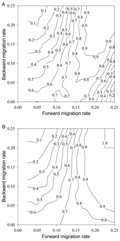
Asymmetry in dispersal influences the likelihood of adaptation to a sink habitat. A, Probability of adaptation of the sink after 1,000 generations of migration, as a function of forward (from the source to the sink) and backward (from the sink to the source) per capita migration rates, in the system of figure 1C. The parameters are fecundity = 4, source and sink K = 128, nμ = 0.01, α² = 0.05, ω² = 1, and sink maladaptation = 3. B, Same as A, except that in order to reduce the impact of density dependence in the sink, we increase the ceiling carrying capacity there to K = 256, while the source K remains at 128. Probabilities were found for migration rates in increments of 0.025 (backward migration could be 0, but not forward migration), and contours at each point were calculated using the four nearest calculated values.

Emigration from the sink, in effect, reduces the realized fitness of residents and also reduces the impact of negative density dependence in the sink, regardless of where emigrants go. So the observed positive effect of emigration back to the source on sink adaptation must reflect a positive effect on the source genetic composition, an effect that more than outweighs the direct fitness loss via emigration and goes beyond the ecological impact of density dependence. Before the sink is adapted, its abundance is low, so it will send few emigrants back to the source. But if the forward-immigration rate is large, then there can be a significant number of survivors of selection, even in a maladapted sink population, some fraction of which (the ordinate in fig. 4) then migrates back to the source. This can easily average several individuals per generation. These individuals have survived selection in the sink and so tend to have alleles better adapted to the sink than do average individuals in the source. These back migrants mate with individuals in the source; this perturbs the genetics of the source population and thus of the pool of sink immigrants, in a way tilted toward aiding adaptation to the sink. More detailed analyses of the time series of adaptation (details not shown) reveal that the coupling with the sink on source population genetics starts to have an effect even before abundance starts to rise substantially in the sink population.

Increasing immigration rates at low levels often facilitates adaptation to the sink in these examples. Overall, whether an increase in dispersal hampers or facilitates adaptation depends on the fate of emigrants, the degree of asymmetry in movement rates, and the impact of density dependence. If emigrants return to the source, this is much better for adaptation than is emigration to the external environment. When the population in the sink is sufficiently large that density dependence is experienced, and emigrants return to the source, the magnitude of the fitness cost of emigration is reduced if local density decreases in the sink, and increased emigration can facilitate adaptation.

Transgressive Evolution in Heterogeneous Landscapes

The final scenario we consider is for a species already adapted to two habitats with different adaptive optima arrayed along a gradient and coupled by dispersal (fig. 1D). The occupied habitats comprise its geographical range. A third habitat is present, but the species initially is too maladapted to persist there without recurrent immigration. This arrangement could describe habitats arrayed along a gradient with localized dispersal (e.g., nearest-neighbor movement). For our Daphnia magna example, one could imagine local adaptation among ponds located along a gradient in bedrock chemistry, with slow-moving streams coupling three water bodies. The question we consider is how the magnitude of heterogeneity and local adaptation in the occupied landscape influences the likelihood of niche evolution permitting its persistence outside its initial range.

Habitats 1 and 2 (fig. 1D) are initially occupied by adapted populations, and stabilizing selection occurs in each with different optima (−d and 0, respectively). Each recipient population receives immigrants that are on average maladapted, relative to local conditions. Hence, each has a mean phenotype displaced from the local adaptive optimum, in the direction of the other habitat. The magnitude of this displacement reflects the blend of gene flow and selection. The sink has conditions outside the species’ niche, but a population is sustained there by recurrent immigration from habitat 2. Using individual-based simulations, we characterized probability of adaptation to the sink over 1,000 generations, as a function of the difference in the phenotypic optima between the two occupied habitats (d), for a fixed difference between the sink and the source of immigrants (habitat 2, in the middle of fig. 1D). As habitat 1 becomes increasingly different from habitat 2 (the source), this should pull the average phenotype in the source habitat in a direction away from the sink optimum, so on average immigrants into the sink should be increasingly maladapted there. Given this, we expected that this should make adaptation to the sink progressively harder, and so the range would be more likely to remain constrained over reasonable time horizons if the species occupies an increasingly heterogeneous landscape.

It turns out that this intuition is only partly correct. As one gradually increases the difference in optima between the occupied habitats, at first it indeed becomes more difficult for adaptation to the sink to occur (fig. 5). But then this trend turns around, and increasing heterogeneity within the occupied range substantially facilitates adaptation to the sink. This nonlinear relationship between the heterogeneity of environments encompassed within the range and the propensity to successfully adapt and colonize beyond the initial range edge holds for a wide range of sink maladaptation (the difference in phenotypic optima between source and sink; fig. 5A) and for one to many genetic loci (fig. 5B). Note that figure 5A is for two-way dispersal coupling all adjacent populations in figure 1D, whereas figure 5B is for unidirectional dispersal, left to right; the pattern is robust to this change in the pattern of dispersal. It also holds for all values of carrying capacities we have examined (in this section, we generally used a modest K to speed up computation, but results at higher K are very similar). Figure 5B shows that for sufficiently high d, the probability of adaptation again begins to drop with increasing d. This is likely because alleles from habitat 1 introduced into habitat 2 are now so maladapted there that they are more or less immediately eliminated by selection and hence have little effect on the source’s genetics. Thus, the probability of adaptation in the sink approaches that which is expected, were the source not coupled to another habitat along the gradient (as in fig. 1C; this is also very close to the probability of adaptation for d = 0, i.e., habitats 1 and 2 having the same optima).

Figure 5.

Transgressive evolution into unoccupied habitats, permitted by local adaptation and migration among occupied sites. A, Probability of adaptation after 1,000 generations of 10% two-way migration between a source at phenotypic optimum = 0 (habitat 2) and a sink at phenotypic optimum given in the key. The source is linked by two-way 10% migration with another adapted population (habitat 1) with phenotypic optimum equal to the negative of the abscissa. There are 10 loci, and 3,000 generations of migration between habitats 1 and 2 elapse before migration to the sink starts. B, Same as A, except that the number of loci is 1, 2, and 10 (given in the key), there is one-way migration (both between adapted populations and to the sink), and the sink maladaptation (phenotypic optimum) = 3. For both A and B, nμ = 0.01, α² = 0.05, ω² = 1, and K = 64.

To interpret this intriguing and unexpected finding (i.e., the increase in adaptation with increasing d), we examined in more detail the genetic details underlying the process of adaptation. Before adaptation, the sink habitat outside the species’ range has few individuals and, to a reasonable approximation, can be ignored in terms of understanding interactions between populations and the emergent genetic structure within the occupied range (for one-way dispersal, of course, the sink never has any effect on the occupied range). The interplay of gene flow and local selection affects not just the average phenotype of potential immigrants into the sink habitat but the entire distributions of genotypic and allelic values available for dispersal (the genotype or genotypic value of an individual refers to the genetic contribution to its phenotype, which is the sum of all its allelic values). We suggest that the impact of gene flow on the entire genotypic distributions, and in particular the prevalence of extreme genotypes, is responsible for the effect shown in figure 5.

We examined the distributions of genotypes and allelic values of an adapted population (habitat 2 in fig. 1D, which we refer to as the recipient source) receiving recurrent migration from another adapted population (habitat 1, which we call the provider source) with a different phenotypic optimum, both with and without back migration. With unidirectional migration, the recipient source population (habitat 2) receives a constant influx of genotypes adapted to the provider source environment (habitat 1), which affects the recipient population’s genetic structure. An example of the probability density functions (PDFs) of genotypic values in the recipient source is shown in figure 6A. This population has a phenotypic optimum of 0, and the key gives the optimum of the provider source (which is −d). If both populations have the same phenotypic optimum (the curve labeled 0), the PDF is very similar to that of a single population with no immigration. Given a difference in phenotypic optima, the mean genotype of the recipient source is pulled toward that of the other habitat. The PDFs of the genotypic values show that if the two habitats have similar optima (d is low), the effect is mostly to shift the entire distribution toward the provider source optimum (to the left). However, for larger d, the distribution broadens significantly and in an asymmetric fashion. There is understandably a fat tail in the distribution in the direction of the provider source (representing the contribution of immigrant alleles). But importantly, the tail of the distribution that is in the opposite direction is also increased.

Figure 6.

Influence of immigration on the distribution of genotypic and allelic values. A, Probability density function (PDF) of the genotype in a population adapted to a habitat (habitat 2 in fig. 1D) with optimum phenotype = 0 and recurrent immigration (one way) of 10% from a population adapted to a habitat (habitat 1) with a different phenotypic optimum (given in the key). The distributions were found by averaging over the entire adult population for 500 generations of each run, for 1,000 independent runs (K = 64, nμ = 0.01, α² = 0.05, ω² = 1, n = 10). B, PDF of allelic values in the recipient population, relative to the average allelic value of the corresponding loci in the sink (calculated each generation), for simulations of panel A.

Before we attempt to explain this effect, note that individuals with genotypes in this upper tail would be less maladapted, were they to move to the sink, than would individuals with the mean genotype of the population (which is pulled away from the sink). If adaptation depends on colonization by rare individuals that by chance are not too maladapted to the sink, an increase in the upper tail of the PDF could account for the increased likelihood of adaptation with increasing d seen in figure 5. (Note that for the larger differences in phenotypic optima shown, 1.5 and above, the genetic distributions tend to become trimodal. This is due to alleles of large effect at one locus, as discussed below.)

As the entire distribution of genotypic values in a focal population is significantly changed by recurrent migration, the distribution of allelic values at various loci must also change. To examine this, we calculated the PDF of the difference between each allelic value in the recipient source and the average value for the corresponding locus of the provider source population, in corresponding generations, averaged over all loci for many generations and many independent simulations. These differences are dominated by a narrow peak around 0, indicating that most recipient population alleles are actually the same or very close in their phenotypic effects to provider source alleles at the same locus (fig. 6B; note the logarithmic scale). For sufficient differences in phenotypic optima, there is also a second prominent peak in the PDF. For these peaks, the recipient source has allelic values higher than corresponding values in the provider source, even though the latter’s phenotypic optimum is lower.

There is a constant infusion into the recipient source of alleles adapted to the provider source, some of which survive even though they degrade adaptation in the recipient. This creates a genetic environment for selection in which some alleles are favored that would not be favored without recurrent immigration. Alleles with strong phenotypic effects of opposite polarity to those common in the provider source, when combined by mating with alleles brought in by immigration from the provider source, can result in an offspring genotype near the recipient habitat’s phenotypic optimum. In other words, if fitness is determined by a polygenic trait with additive genetic effects, gene flow can foster the retention of a small pool of alleles with relatively extreme phenotypic effects in the opposite direction of the provider source population. If by chance individuals with these alleles immigrate to the sink, they will have a higher average initial fitness there than expected from the average phenotype of their population. We suggest that this accounts for the effect shown in figure 5.

To examine the effects of gene flow on genetic architecture further, we calculated the difference between average provider and recipient source allelic values at each locus through time, for 10% one-way recurrent immigration and 10 loci (fig. 7A). After migration starts, there is a period of about 500 generations during which there are differences at several loci, then 500 generations with significant differences at two loci, before the difference becomes confined to one locus, after which it tends to remain in this state. Therefore, the upper peaks in the PDFs of figure 6B are likely due to alleles at a single locus for each population (the difference in phenotypic optima for fig. 7A is 2.5). Alleles at nine loci follow the provider source, with alleles at the other locus deviating sharply in the other direction. A comparable pattern emerges by generation 3,000 over multiple independent runs: most of the genetic differences between the source and the recipient populations are concentrated in a single locus. The pattern can be seen more clearly by examining a two-locus model for which the average allelic values at each locus for each population can be shown (fig. 7A shows only the provider-recipient population differences at each locus and has 10 curves, most of which overlap around 0). In figure 7B (with two loci), one-way dispersal starts at generation 0, before which the provider source alleles are near −0.6 (its optimum is −2.5, and there are four alleles per individual) and the recipient source alleles are near 0 (its optimum). Shortly after dispersal starts, locus 2 in the recipient population moves toward locus 2 of the provider source (and then tracks it), while recipient locus 1 moves in the opposite direction.

Figure 7.

Changes in genetic architecture resulting from the interplay of gene flow and selection. A, Difference between source and recipient populations in mean allelic value at each of 10 loci over 3,000 generations under the conditions of figure 6, with source and recipient differing in phenotypic optimum by 2.5. For the first 500 generations, there are significant differences at several loci, then from generations 500 to 1,000 at only two loci, and after that at only one locus. B, Time plots of average allelic values at both loci (one locus in solid lines, the other dashed lines) in two populations (source, thin lines; recipient, thick lines) in a two-locus model. One-way 10% migration from the source to the recipient population starts at generation 0. Phenotypic optima are −2.5 for the source and 0 for the recipient population; K = 64, and other parameters are as in figure 6.

As has been long known, if one subjects two populations to stabilizing selection with different optima, and then crosses them, the resultant hybrid population has a greater genetic variance than either parental population. This straightforward effect, however, does not explain the patterns we see, which only emerge gradually over time with recurrent migration and often involve differences concentrated at one or a few loci. A change in genetic architecture in effect occurs in some cases in our models as species evolve in their niche to utilize sink habitats. An analytic understanding of this phenomenon would require an explicit formal analysis of the interplay of selection, gene flow, and drift in a multilocus context, which goes beyond what we are aiming at in this article. But some phenomenological observations arising from our simulations may be useful in moving toward such an analysis. As figure 7A shows, initially the genetic difference between populations is spread over a number of loci. But each increase in the difference at one locus reduces the selection leading to larger differences at other loci (or can cause selection leading to smaller differences). All loci have a continual influx of provider source alleles. So we conjecture that having the difference concentrated at one locus is a more stable solution, given that all other alleles just converge in value to those of the source. The one locus that is very different between the two populations then continues to experience strong selection against the source alleles. Were the differences between the populations spread over many loci, it would be more difficult to maintain the differences, leading to constant shifting as to which loci are different; this indeed appears to be what is happening shortly after immigration is initiated in figure 7A. It is notable in our simulations that the locus that initially has the largest differentiation need not be the one sustaining the largest difference in the long run. This doubtless reflects the chance vicissitudes of which loci happen to pick up favorable mutations, which is not guaranteed to be the locus that initially showed the greatest differentiation.

We should note that these interesting effects at the genetic level are most notable when there is a low mutation rate, so heritability is low (details not shown). At higher mutation rates, much less of the genetic difference between the two populations is focused at a single locus. Yet the nonlinear pattern shown in figure 5, relating heterogeneity in the occupied range to the rate of adaptive colonization outside of it, qualitatively continues to hold even with higher mutation.

Different evolutionary results might arise for different landscape structures. If instead of the sink being beyond the margin of the occupied range along a gradient (as in fig. 1D), for historical reasons it might happen to be intermediate in both space and its local optimum. So along the phenotype axis, source 1 might have optimum −d, the middle habitat (the sink) optimum 0, and source 2 an optimum of −d, with both sources providing immigrants to the sink. Measured against the source-sink scenario of figure 1C (see fig. 3C), adaptation to the sink via selection on a quantitative trait should now happen quite rapidly in sexual species. The reason is that mixed matings from the two sources produce offspring with intermediate phenotypes that should be well-adapted to the sink. In other words, “holes” in a sexual species’ niche might be expected to be rapidly filled. By contrast, if the three habitats are arranged as in figure 1D and have optima −d, 0, and then again −d (the sink), local adaptation to the middle habitat itself might at first glance be expected to slow further expansion of the species, if dispersal is restricted to nearest neighbors (a reviewer suggested this possibility to us). However, note that there are large tails on both sides of the genotypic distribution in figure 6A, with a particularly fat tail in the direction of the source population. Therefore, adaptation to the sink can be facilitated in this case, because the middle population contains a substantial pool of genotypes expected to have reasonable fitness when put into the sink. These different potential outcomes of range evolution reflect again the insight of Caughley et al. (1988) that range limits reflect the “geographic facts of environment.”

Discussion

Understanding why range limits are stable, over short to long timescales, has been a long-standing objective of ecology and evolutionary biology. A full understanding of both stable and unstable range dynamics, we suggest, requires analysis of the interplay of demographic and evolutionary processes, in the context of particular landscapes. In this article, we have not attempted to provide a comprehensive review of the entire literature, which has been the focus of a number of excellent reviews recently and is in any case growing rapidly. Instead, we have used simplified spatial scenarios (see fig. 1) and individual-based models of coupled demography and evolution to bring out general issues that we believe cut across many of the details of particular models and systems. We have suggested that there is an intimate relationship between the range limit issue and understanding more broadly the evolution of species’ niches. There is growing interest in comprehending the causes and consequences of niche conservatism, versus niche evolution, in heterogeneous environments (Futuyma 2010; Wiens et al. 2010), and studies of range limits provide one potential arena for testing many proposed theories.

The reason the studies of ranges and niches are not essentially synonymous is that ranges reflect the history of dispersal as well as niche requirements. When dispersal is limited, suitable habitat may not be occupied because of dispersal barriers (Pulliam 2000). Conversely, habitats may be outside the niche yet occupied (even at high abundance) because of high rates of dispersal maintaining sink populations. If dispersal occurs episodically, an island biogeographic or metapopulation perspective on range limits may be particularly germane. We first sketched models showing that given dispersal pulses into habitats outside the niche, in general one expects to see extinction rather than evolution, unless the number of colonizing individuals is large and the initial growth rate is not too low. If biogeographic ranges are influenced in large measure by an occasional trickle of dispersers arriving in new locations at low numbers, we would expect species to tend to occupy ranges with habitats already within their niche, rather than to frequently invade outside. The basic reason is that extinction readily overwhelms evolution during colonization attempts outside the niche.

With recurrent immigration, we have suggested that a number of new issues arise. In addition to providing a fresh supply of genetic variation, immigrants can also maintain populations for which density dependence becomes important (which can make adaptation more difficult) and, in sexual, randomly mating species, can further impose a migrational load on the resident population. Our individual-based models show that which of these effects predominates may depend on details such as the ordering of events in the life history, the effect of density dependence at ambient population levels in the sink, and underlying rates of mutation. When descendents of emigrants end up back in the original source, spatial feedback effects can arise, such that intermediate rates of movement in each direction may often facilitate adaptation to the sink. Expanding spatial models to include asymmetric patterns of movement, rather than simply assuming simple diffusion-like movement patterns, may provide novel insights into both the statics and the dynamics of species ranges.

The effect of dispersal on genetic variation is particularly important. Gene flow along gradients with spatially varying selection can pump up variation, relaxing constraints on adaptation along the gradient (Barton 2001; Polechova et al. 2009). This effect can be weakened by stochastic processes in low-density populations at range margins (Bridle et al. 2010). In our models of niche evolution in discrete habitats, such stochasticity can lead to long transient phases during which a species remains restricted in its range in a kind of quasi-stable equilibrium. Our observation that gene flow can alter the genetic architecture underlying differences between populations in a quantitative trait is not new, although our application of this observation appears to be. Griswold (2006), for instance, carried out simulation studies of a quantitative trait for which selection was on fecundity and mutation was described by a symmetrical, back-to-back distribution of mutational effects at each of a large number of loci. He showed that as migration increased, alleles of larger magnitude in their effect accounted for proportionally more of the phenotypic differences between populations. Although our model makes different assumptions, we too find that genetic architecture changes with recurrent immigration. Thus, the genetic architecture underlying trait variation within and among populations may itself reflect the interplay of selection and dispersal in heterogeneous landscapes. One surprising (to us) consequence is that heterogeneity within a species’ initial occupied range may facilitate its evolutionary scope for further expansion outside that range. The reason is that the interplay of selection and gene flow within populations alters the entire distributions of genotypes available for sampling by emigration and may increase the number of individuals found in a fattened tail, who are incidentally more likely to be able to found populations outside the range of habitats already occupied by the species. In general, the details of genetic architecture and the magnitude of the phenotypic effect of likely mutations appear to matter greatly in range dynamics (Kawecki 2000, 2008; Gomulkiewicz et al. 2010; Kimbrell 2010; Turner and Wong 2010). This is particularly likely if adaptive evolution permitting persistence requires adaptation to multiple distinct ecological factors, where genetic correlations can constrain evolution (Blows and Hoffmann 2004; Hellmann and Pineda-Krch 2007; Gomulkiewicz and Houle 2009; Walsh and Blows 2009).

All of these issues, we suggest, should be revisited across a broader landscape of models. For instance, we have assumed that dispersal rates are fixed, but selection can also act on dispersal itself, with ramifying secondary effects on the likelihood of local adaptation and evolutionarily stable range limits (Rowell 2009). Organisms that can adaptively choose habitats can thereby make evolution less likely to craft adaptation to low-fitness habitats and so indirectly constrain range limits. Conversely, if phenotypic plasticity or learning makes organisms less poorly adapted to a given habitat, the evolution of adaptations permitting persistence there can be facilitated (Chevin and Lande 2009; Levin 2009; Sutter and Kawecki 2009). Alternative assumptions about movement may make it more or less likely that range evolution depends, say, on genes of minor versus major effect.

The above models treat the environment as an unchanging template against which evolution unfolds. But environments change through time, and understanding range limits will ultimately require grappling with temporal as well as spatial variation. Moreover, organisms alter their environments and thereby shift the milieu of evolution (Odling-Smee et al. 2003). Such effects have been almost entirely ignored in the literature on ecological and evolutionary determinants of range limits (Holt 2009). Most species are influenced by interactions with other species, leading in some situations to constraints on evolution of habitat use and range limits (e.g., Holt 1990; De Mazancourt et al. 2008; Price and Kirkpatrick 2009). Conversely, in other cases, interspecific interactions can cause rapid shifts in species’ distributions (to both shrink and expand them), beyond that expected from single species dynamics alone (Nuismer and Kirkpatrick 2003; Case et al. 2005; Moorcroft et al. 2006; Antonovics 2009; Holt and Barfield 2009; Van der Putten et al. 2010), and can at times hamper niche evolution (Holt 1990; De Mazancourt et al. 2008). When a single species splits into two, what happens to its subsequent ranges should depend in part on the role of ecology in speciation itself. For instance, consider a peripheral population constrained in its ability to adapt because of gene flow from a central population (what we might call a “Mayrian” range limit). Once this population does adapt, it should experience selection for reproductive isolation precluding mating with maladapted immigrants (Antonovics 1976). If the range limit of the ancestral species along a gradient had been hampered by gene flow, breaking gene flow could allow continued expansion by the new species along the gradient, whereas back expansion might be precluded by the established presence of its sister species. Conversely, if there is sympatric speciation associated with local ecological differentiation, an open question is the degree to which this local coexistence translates into coexistence across broader spatial scales. The interplay of community ecology, speciation theory, and range theory is just beginning to be developed (McPeek 2007) but will doubtless prove key for understanding the statics and dynamics of species’ ranges.

The interplay of ecology and evolutionary processes can lead to shrinking, as well as expansion, of species’ ranges. We have not emphasized this in the results we have presented, but in some cases species can initially be habitat generalists but lose their adaptations to particular habitats. In some cases, this can be due to gene flow (as in migrational meltdown; Ronce and Kirkpatrick 2001), and this evolutionary trimming of the niche can be reinforced by strong density dependence at low densities (Gomulkiewicz et al. 1999). Another nonadaptive process that can lead to evolutionary habitat loss is the accumulation of locally deleterious mutations in habitats where a species is low in abundance to start with because selection is less effective at weeding such mutants out of populations (Kawecki et al. 1997). Selective forces can also more directly lead to range shrinkage when there are trade-offs in performance across space because selection can in effect “weight” habitats differently. In some situations, natural selection tends to be automatically biased toward habitats that are abundantly, rather than sparsely, occupied or where fitness is greater (as in source-sink dynamics; Holt and Gaines 1992; Kawecki 1995, 2008; Holt 2003; Cohen 2006). In others, the functional form of the trade-off in performance across space itself favors the evolution of habitat specialization (Holt 2003), and selection actively eliminates certain habitats from the spatial repertoire of a species. Given frequency-dependent interactions among individuals, populations even can be driven toward extinction by selection in a kind of “evolutionary suicide” (Webb 2003; Rankin and López-Sepulcre 2005; Burt and Trivers 2006). If the conditions favoring such “suicide” vary across space, range limits might arise for reasons very different from explanations based on failure to adapt to the external environment.

Theoretical studies have made great strides toward providing an answer to Mayr’s puzzle, but the answer turns out to be more subtle and complex than simply the swamping of local adaptation by recurrent gene flow from central to peripheral populations. And there is much left to do. Given the importance of understanding range limits as a component of global change, we see an urgent need for the development of models of coupled evolutionary and demographic dynamics, along the general lines of those we have presented but tied much more closely to the biology of particular species in concrete environmental settings (Angilletta 2009). A nice example of a step toward such a tailored theory of evolutionary rescue and range limits has recently been provided by Kearney et al. (2009), who combine physiological models and evolutionary theory to make predictions about how the range of the dengue mosquito Aedes aegypti is likely to adjust to climate change. In addition to the practical utility of such models for gauging the evolutionary dimensions of biotic responses to global change, we suggest that such models will provide powerful testing grounds for general evolutionary theory on the statics and dynamics of species’ borders.

APPENDIX. An Individual-Based Model for Analyzing Niche Evolution

The model tracks each individual and its genotype in an environment composed of several discrete habitats, one or more of which initially has conditions outside the species’ niche (i.e., a sink habitat at the edge of a species’ range). We assume a diploid population with discrete generations. There is stabilizing selection on a quantitative trait determining the probability of juvenile to adult survival with different phenotypic optima among habitats (see inset in fig. 3C) and fixed adult fecundity. We mainly consider a flow of life-history events that starts with birth, followed by selection on survival, adult migration, density dependence, and finally random mating to produce the next generation (although in the text, we briefly consider an alternative ordering of life-history events).

Genetic variation is depleted by selection and drift and replenished by mutation, so heritability of the trait experiencing selection can vary rather than be fixed. As in earlier publications (e.g., Holt et al. 2003, 2004b), the individual-based simulations rely on the same basic assumptions as those used by Bürger and Lynch (1995), who studied adaptation to a continually changing environment for a single character determined by additive genetic variation at multiple loci. The key genetic assumptions are as follows. There are n additive loci, with no dominance or epistasis, and free recombination; each allele contributes a fixed amount to the individual’s realized phenotype, which is the sum of these allelic values over all n loci plus a Gaussian environmental term with unit variance. Mutational input maintains variation (assuming the “continuum-of-alleles” model). Mutations occur in each generation with a probability of nμ (generally 1%) per haplotype per generation; the mutational effects (added to the previous allelic value) have a Gaussian distribution, with a mean of 0 and variance of α² (typically 0.05 in our simulations). Most mutations have a small effect on the phenotype and fitness, but mutants of large effect can occasionally occur. Our standard assumptions produce an average genetic variance and heritability of about 0.06, although we sometimes use a high-mutation rate giving higher values (heritability around 0.25). This does not alter our qualitative conclusions.

Initially, the species is adapted to one or more source habitats and not present in the sink. We allow the source habitats to evolve over 1,000 generations (or 3,000 generations for the fig. 1D scenario), so as to reach demographic and evolutionary equilibrium. At this phenotypic near-equilibrium, there is an underlying churning at the genetic level, due to the interplay of mutation, drift, and selection. Thus, a continual supply of novel variants arises, which can be “tested” in the sink. After this initialization, we start dispersal, which may be either episodic or recurrent (at a constant per capita rate among habitats), and repeat the simulations for 400 sinks for each parameter set (unless otherwise indicated). Migrants into the sink tend to be maladapted, to a degree that depends on the difference in phenotypic optima between the source and the sink (which we refer to as the sink maladaptation, θ). Because we are focusing on conditions outside the species’ niche, the sink populations tend to be at low abundance (for low to moderate immigration rates), and so genetic variation can be depleted by drift, which can slow the response to selection (Willi et al. 2006).

We assume a “ceiling” form of density dependence, which limits the number of reproducing adults to a carrying capacity K_i for habitat i; growth is density independent if there are fewer adults. If there are more than K_i adults after immigration, K_i individuals are sampled with-out replacement from the pool of available adults to mate as females. For each, a random adult is chosen (with replacement) to act as male. This mating system avoids an Allee effect at low densities (see below). Individuals produce gametes, some of which may carry mutations. Each mated pair produces f offspring, surviving to adulthood with probability exp {− (z − z_i)²/2ω²}, where z is the realized phenotype of a given individual, z_i is the optimum phenotype in habitat i, and ω² is inversely proportional to the strength of stabilizing selection. (The sink maladaptation θ is the difference between source and sink z_i.) This is the stage at which selection occurs. If the average z value is too far from the optimum, mean fitness is below 1, and the population tends to decline. Individuals surviving mortality are adults and either stay in their natal habitat or migrate to another habitat with some fixed probability.

In this individual-based model, stochasticity enters in several ways. At the genetic level, mutation is stochastic. Immigrants to the sink have multilocus allelic combinations that vary because of random sampling. Finally, because survival is probabilistic, there is both genetic drift and chance variation in population size. We defined a sink population as “adapted” if its average genotype at the end of a simulation was closer to the sink optimum than it was to the source optimum. We can also define a sink to be adapted if its average fitness is greater than 1. This leads to very similar results (not shown). For populations that are adapted by these criteria, persistence is likely if immigration is discontinued. With adult migration and a moderate mutation rate (1% per haplotype), we previously reported a small positive effect of an increasing migration rate on adaptation (Holt et al. 2003). However, those results assumed a monogamous mating system with fixed average fecundity per mating pair. Monogamous mating with fixed average fecundity per pair introduces a small Allee effect for low population sizes, because when the population size is an odd number, one individual does not mate. In general, with Allee effects, an increase in immigration increases fitness at low abundances, which facilitates adaptation in a wide range of models (Holt et al. 2004a). When this Allee effect is removed, the migration rate still has an effect, but it is rather modest and depends in magnitude and direction on how severe the sink is and the overall level of genetic variation maintained by mutation in the source. The mating system used here, as described above, avoids this Allee effect.

Literature Cited

- Alleaume-Benharira M, I, Pen R, Ronce O. Geographical patterns of adaptation within a species’ range: interactions between drift and gene flow. Journal of Evolutionary Biology. 2006;19:203–215. doi: 10.1111/j.1420-9101.2005.00976.x. [DOI] [PubMed] [Google Scholar]
- Anderson JT, Geber MA. Demographic source-sink dynamics restrict local adaptation in Elliott’s blueberry (Vaccinium elliottii) Evolution. 2010;64:370–384. doi: 10.1111/j.1558-5646.2009.00825.x. [DOI] [PubMed] [Google Scholar]
- Andrewartha HG, Birch LC. The distribution and abundance of animals. University of Chicago Press; Chicago: 1954. [Google Scholar]
- Angert AL, Bradshaw HD, Jr, Schemske DW. Using experimental evolution to investigate geographic range limits in monkeyflowers. Evolution. 2008;62:2660–2675. doi: 10.1111/j.1558-5646.2008.00471.x. [DOI] [PubMed] [Google Scholar]
- Angilletta MJ., Jr . Thermal adaptation: a theoretical and empirical synthesis. Oxford University Press; Oxford: 2009. [Google Scholar]
- Antia R, Regoes RR, Koella JC, Bergstrom CT. The role of evolution in the emergence of infectious diseases. Nature. 2003;426:658–661. doi: 10.1038/nature02104. [DOI] [PMC free article] [PubMed] [Google Scholar]
- Antonovics J. The nature of limits to natural selection. Annals of the Missouri Botanical Garden. 1976;63:224–247. [Google Scholar]
- Antonovics J. The effect of sterilizing disease on host abundance and distribution along environmental gradients. Proceedings of the Royal Society B: Biological Sciences. 2009;276:1391–1534. doi: 10.1098/rspb.2008.1256. [DOI] [PMC free article] [PubMed] [Google Scholar]
- Antonovics J, McKane AJ, Newman TJ. Spatiotemporal dynamics in marginal populations. American Naturalist. 2006;167:16–27. doi: 10.1086/498539. [DOI] [PubMed] [Google Scholar]
- Bakker J, van Rijswijk MEC, Weissing FJ, Bijlsma R. Consequences of fragmentation for the ability to adapt to novel environments in experimental Drosophila metapopulations. Conservation Genetics. 2010;11:435–448. [Google Scholar]
- Barton N. Adaptation at the edge of a species’ range. In: Silvertown J, Antonovics J, editors. Integrating ecology and evolution in a spatial context. Blackwell; Oxford: 2001. pp. 365–392. [Google Scholar]
- Beddington JR, Free CA, Lawton JH. Concepts of stability and resilience in predator-prey models. Journal of Animal Ecology. 1976;45:791–816. [Google Scholar]
- Bell G. Selection: the mechanism of evolution. 2. Oxford University Press; Oxford: 2008. [Google Scholar]
- Bell G, Collins S. Adaptation, extinction and global change. Evolutionary Applications. 2008;1:3–16. doi: 10.1111/j.1752-4571.2007.00011.x. [DOI] [PMC free article] [PubMed] [Google Scholar]
- Bell G, Gonzalez A. Evolutionary rescue can prevent extinction following environmental change. Ecology Letters. 2009;12:942–948. doi: 10.1111/j.1461-0248.2009.01350.x. [DOI] [PubMed] [Google Scholar]
- Bell G, Lechowicz MJ, Appenzeller A, Chandler M, DeBlois E, Jackson L, Mackenzie B, Preziosi R, Schallenberg M, Tinker N. The spatial structure of the physical environment. Oecologia (Berlin) 1993;96:114–121. doi: 10.1007/BF00318038. [DOI] [PubMed] [Google Scholar]
- Blows MW, Hoffmann AA. A reassessment of genetic limits to evolutionary change. Ecology. 2004;86:1371–1384. [Google Scholar]
- Bolnick DI, Nosil P. Natural selection in populations subject to a migration load. Evolution. 2007;61:2229–2243. doi: 10.1111/j.1558-5646.2007.00179.x. [DOI] [PubMed] [Google Scholar]
- Bradshaw AD. The importance of evolutionary ideas in ecology—and vice versa. In: Schorrocks B, editor. Evolutionary ecology. Blackwell; Oxford: 1984. pp. 1–25. [Google Scholar]
- Bradshaw AD. The Croonian lecture, 1991: genostasis and the limits to evolution. Philosophical Transactions of the Royal Society B: Biological Sciences. 1991;333:289–305. doi: 10.1098/rstb.1991.0079. [DOI] [PubMed] [Google Scholar]
- Bridle JR, Vines TH. Limits to evolution at range margins: when and why does adaptation fail? Trends in Ecology & Evolution. 2007;22:140–147. doi: 10.1016/j.tree.2006.11.002. [DOI] [PubMed] [Google Scholar]
- Bridle J, Polechova J, Kawata M, Butlin RK. Why is adaptation prevented at ecological margins? new insights from individual-based simulations. Ecology Letters. 2010;13:485–494. doi: 10.1111/j.1461-0248.2010.01442.x. [DOI] [PubMed] [Google Scholar]
- Bürger R, Lynch M. Evolution and extinction in a changing environment: a quantitative-genetic analysis. Evolution. 1995;49:151–163. doi: 10.1111/j.1558-5646.1995.tb05967.x. [DOI] [PubMed] [Google Scholar]
- Burt A, Trivers R. Genes in conflict. Harvard University Press; Cambridge, MA: 2006. [Google Scholar]
- Carter RN, Prince SD. Epidemic models used to explain biogeographical distribution-limits. Nature. 1981;293:644–645. [Google Scholar]
- Case TJ, Taper ML. Interspecific competition, gene flow, and the coevolution of species borders. American Naturalist. 2000;155:583–605. doi: 10.1086/303351. [DOI] [PubMed] [Google Scholar]
- Case TJ, Holt RD, McPeek MA, Keitt TH. The community context of species borders: ecological and evolutionary perspectives. Oikos. 2005;108:18–27. [Google Scholar]
- Caughley G, Grice D, Barker R, Brown B. The edge of the range. Journal of Animal Ecology. 1988;57:771–785. [Google Scholar]
- Chase JM, Leibold MA. Ecological niches: linking classical and contemporary approaches. University of Chicago Press; Chicago: 2003. [Google Scholar]
- Chevin L, Lande R. When do adaptive plasticity and genetic evolution prevent extinction of a density-regulated population? Evolution. 2009;64:1143–1150. doi: 10.1111/j.1558-5646.2009.00875.x. [DOI] [PubMed] [Google Scholar]
- Cohen D. Modeling the evolutionary and ecological consequences of selection and adaptation in heterogeneous environments. Israel Journal of Ecology and Evolution. 2006;52:467–484. [Google Scholar]
- Crawford RMM. Plants at the margin: ecological limits and climate change. Cambridge University Press; Cambridge: 2008. [Google Scholar]
- De Mazancourt C, Johnson E, Barraclough TG. Bio-diversity inhibits species’ evolutionary responses to changing environments. Ecology Letters. 2008;11:380–388. doi: 10.1111/j.1461-0248.2008.01152.x. [DOI] [PubMed] [Google Scholar]
- Eckhart VM, Geber MA, Morris WF, Fabio ES, Tiffin P, Moeller DA. The geography of demography: long-term demographic studies and species distribution models reveal a species border limited by adaptation. American Naturalist. 2011;178(suppl):S26–S43. doi: 10.1086/661782. [DOI] [PubMed] [Google Scholar]
- Filin I, Holt RD, Barfield M. The relation of density regulation to habitat specialization, evolution of a species’ range, and the dynamics of biological invasions. American Naturalist. 2008;172:233–247. doi: 10.1086/589459. [DOI] [PubMed] [Google Scholar]
- Futuyma DJ. Evolutionary constraint and ecological consequences. Evolution. 2010;64:1865–1884. doi: 10.1111/j.1558-5646.2010.00960.x. [DOI] [PubMed] [Google Scholar]
- Gallagher RV, Beaumont LJ, Hughes L, Leishman MR. Evidence for climatic niche and biome shifts between native and novel ranges in plant species introduced to Australia. Journal of Ecology. 2010;98:790–799. [Google Scholar]
- Garcia-Ramos G, Kirkpatrick M. Genetic models of adaptation and gene flow in peripheral populations. Evolution. 1997;51:21–28. doi: 10.1111/j.1558-5646.1997.tb02384.x. [DOI] [PubMed] [Google Scholar]
- Gaston KJ. The structure and dynamics of geographic ranges. Oxford University Press; Oxford: 2003. [Google Scholar]
- Gaston KJ. Geographic range limits: achieving synthesis. Proceedings of the Royal Society B: Biological Sciences. 2009;276:1395–1406. doi: 10.1098/rspb.2008.1480. [DOI] [PMC free article] [PubMed] [Google Scholar]
- Gomulkiewicz R, Holt RD. When does evolution by natural selection prevent extinction? Evolution. 1995;49:201–207. doi: 10.1111/j.1558-5646.1995.tb05971.x. [DOI] [PubMed] [Google Scholar]
- Gomulkiewicz R, Houle D. Demographic and genetic constraints on evolution. American Naturalist. 2009;174:218–229. doi: 10.1086/645086. [DOI] [PubMed] [Google Scholar]
- Gomulkiewicz R, Holt RD, Barfield M. The effects of density dependence and immigration on local adaptation in a black-hole sink environment. Theoretical Population Biology. 1999;55:283–296. doi: 10.1006/tpbi.1998.1405. [DOI] [PubMed] [Google Scholar]
- Gomulkiewicz R, Holt RD, Barfield M, Nuismer SL. Genetics, adaptation, and invasion in harsh environments. Evolutionary Applications. 2010;3:97–108. doi: 10.1111/j.1752-4571.2009.00117.x. [DOI] [PMC free article] [PubMed] [Google Scholar]
- Griswold CK. Gene flow’s effect on the genetic architecture of a local adaptation and its consequences for QTL analyses. Heredity. 2006;96:445–453. doi: 10.1038/sj.hdy.6800822. [DOI] [PubMed] [Google Scholar]
- Hebert PDN, Finster TL. Macrogeographic patterns of breeding system diversity in the Daphnia pulex group for the United States and Mexico. Heredity. 2001;87:153–161. doi: 10.1046/j.1365-2540.2001.00885.x. [DOI] [PubMed] [Google Scholar]
- Hellmann JJ, Pineda-Krch M. Constraints and reinforcement on adaptation under climate change: selection of genetically correlated traits. Biological Conservation. 2007;137:599–609. [Google Scholar]
- Hochberg ME, Ives AR. Can natural enemies enforce geographical range limits? Ecography. 1999;22:268–276. [Google Scholar]
- Holt RD. Immigration and the dynamics of peripheral populations. In: Miyata K, Rhodin A, editors. Advances in herpetology and evolutionary biology. Harvard University Press; Cambridge, MA: 1983. pp. 680–694. [Google Scholar]
- Holt RD. The microevolutionary consequences of climate change. Trends in Ecology & Evolution. 1990;5:311–315. doi: 10.1016/0169-5347(90)90088-U. [DOI] [PubMed] [Google Scholar]
- Holt RD. Demographic constraints in evolution: towards unifying the evolutionary theories of senescence and niche conservatism. Evolutionary Ecology. 1996;10:1–11. [Google Scholar]
- Holt RD. On the evolutionary ecology of species ranges. Evolutionary Ecology Research. 2003;5:159–178. [Google Scholar]
- Holt RD. Bringing the Hutchinsonian niche into the 21st century: ecological and evolutionary perspectives. Proceedings of the National Academy of Sciences of the USA. 2009;106:19659–19665. doi: 10.1073/pnas.0905137106. [DOI] [PMC free article] [PubMed] [Google Scholar]
- Holt RD, Barfield M. Trophic interactions and range limits: the diverse roles of predation. Proceedings of the Royal Society B: Biological Sciences. 2009;276:1435–1442. doi: 10.1098/rspb.2008.1536. [DOI] [PMC free article] [PubMed] [Google Scholar]
- Holt RD, Gaines MS. Analysis of adaptation in heterogeneous landscapes: implications for the evolution of fundamental niches. Evolutionary Ecology. 1992;6:433–447. [Google Scholar]
- Holt RD, Gomulkiewicz R. The evolution of species’ niches: a population dynamic perspective. In: Othmer H, Adler F, Lewis M, Dallon J, editors. Case studies in mathematical modelling: ecology, physiology, and cell biology. Prentice-Hall; Englewood Cliffs, NJ: 1997a. pp. 25–50. [Google Scholar]
- Holt RD, Gomulkiewicz R. How does immigration influence local adaptation? a reexamination of a familiar paradigm. American Naturalist. 1997b;149:563–572. [Google Scholar]
- Holt RD, Keitt T. Alternative causes for range limits: a metapopulation perspective. Ecology Letters. 2000;3:41–47. [Google Scholar]
- Holt RD, Gomulkiewicz R, Barfield M. The phenomenology of niche evolution via quantitative traits in a “black-hole” sink. Proceedings of the Royal Society B: Biological Sciences. 2003;270:215–224. doi: 10.1098/rspb.2002.2219. [DOI] [PMC free article] [PubMed] [Google Scholar]
- Holt RD, Knight TM, Barfield M. Allee effects, immigration, and the evolution of species’ niches. American Naturalist. 2004a;163:253–262. doi: 10.1086/381408. [DOI] [PubMed] [Google Scholar]
- Holt RD, Gomulkiewicz R, Barfield M. Temporal variation can facilitate niche evolution in harsh sink environments. American Naturalist. 2004b;164:187–200. doi: 10.1086/422343. [DOI] [PubMed] [Google Scholar]
- Holt RD, Keitt T, Lewis M, Maurer B, Taper M. Theoretical models of species’ borders: single species approaches. Oikos. 2005a;108:28–46. [Google Scholar]
- Holt RD, Barfield M, Gomulkiewicz R. Theories of niche conservatism and evolution: could exotic species be potential tests? In: Sax DF, Gaines SD, Stachowicz JJ, editors. Species invasions: insights to ecology, evolution and biogeography. Sinauer; Sunderland, MA: 2005b. pp. 259–290. [Google Scholar]
- Hooper HL, Connon R, Callaghan A, Fryer G, Yarwood-Buchanan S, Biggs J, Maund SJ, Hutchinson TH, Sibly RM. The ecological niche of Daphnia magna characterized using population growth rate. Ecology. 2008;89:1015–1022. doi: 10.1890/07-0559.1. [DOI] [PubMed] [Google Scholar]
- Hutchinson GE. An introduction to population ecology. Yale University Press; New Haven, CT: 1978. [Google Scholar]
- Jump AS, Peñuelas J. Running to stand still: adaptation and the response of plants to rapid climate change. Ecology Letters. 2005;8:1010–1020. doi: 10.1111/j.1461-0248.2005.00796.x. [DOI] [PubMed] [Google Scholar]
- Kawecki TJ. Demography of source-sink populations and the evolution of ecological niches. Evolutionary Ecology. 1995;9:38–44. [Google Scholar]
- Kawecki TJ. Adaptation to marginal habitats: contrasting influence of dispersal on the fate of rare alleles with small and large effects. Proceedings of the Royal Society B: Biological Sciences. 2000;267:113–130. doi: 10.1098/rspb.2000.1144. [DOI] [PMC free article] [PubMed] [Google Scholar]
- Kawecki TJ. Ecological and evolutionary consequences of source-sink population dynamics. In: Hanski I, Gaggiotti OE, editors. Ecology, genetics and evolution of metapopulations. Academic Press; Oxford: 2004. pp. 387–414. [Google Scholar]
- Kawecki TJ. Adaptation to marginal habitats. Annual Review of Ecology, Evolution, and Systematics. 2008;39:321–342. [Google Scholar]
- Kawecki TJ, Holt RD. Evolutionary consequences of asymmetric dispersal rates. American Naturalist. 2002;160:333–347. doi: 10.1086/341519. [DOI] [PubMed] [Google Scholar]
- Kawecki TJ, Barton NH, Fry JD. Mutational collapse of fitness in marginal habitats and the evolution of ecological specialization. Journal of Evolutionary Biology. 1997;10:407–429. [Google Scholar]
- Kearney M, Porter WP, Williams C, Ritchie S, Hoffmann AA. Integrating biophysical models and evolutionary theory to predict climatic impacts on species’ ranges: the dengue mosquito Aedes aegypti in Australia. Functional Ecology. 2009;23:528–538. [Google Scholar]
- Keitt TH, Lewis MA, Holt RD. Allee dynamics, critical phenomena, and species’ borders. American Naturalist. 2001;157:203–216. doi: 10.1086/318633. [DOI] [PubMed] [Google Scholar]
- Kellerman V, van Heerwaarden B, Sgro CM, Hoffmann AA. Fundamental evolutionary limits in ecological traits drive Drosophila species distributions. Science. 2009;325:1244–1246. doi: 10.1126/science.1175443. [DOI] [PubMed] [Google Scholar]
- Kimbrell T. Canalization and adaptation in a landscape of sources and sinks. Evolutionary Ecology. 2010;24:891–909. [Google Scholar]
- Kinnison MT, Hairston NG., Jr Eco-evolutionary conservation biology: contemporary evolution and the dynamics of persistence. Functional Ecology. 2007;21:444–454. [Google Scholar]
- Kirkpatrick M, Barton NH. Evolution of a species’ range. American Naturalist. 1997;150:1–23. doi: 10.1086/286054. [DOI] [PubMed] [Google Scholar]
- Kunin WE, Vergeer P, Kenta T, Davey MP, Burke T, Woodward FI, Quick P, Mannarelli ME, Watson-Haigh NS, Butlin R. Variation at range margins across multiple spatial scales: environmental temperature, population genetics and metabolomic phenotype. Proceedings of the Royal Society B: Biological Sciences. 2009;276:1495–1507. doi: 10.1098/rspb.2008.1767. [DOI] [PMC free article] [PubMed] [Google Scholar]
- Levin DA. Flowering-time plasticity facilitates niche shifts in adjacent populations. New Phytologist. 2009;183:661–666. doi: 10.1111/j.1469-8137.2009.02889.x. [DOI] [PubMed] [Google Scholar]
- Lynch M, Lande R. Evolution and extinction in response to environmental change. In: Kareiva PM, Kingsolver JG, Huey RB, editors. Biotic interactions and global change. Sinauer; Sunderland, MA: 1993. pp. 234–250. [Google Scholar]
- Mayr E. Animal species and evolution. Harvard University Press; Cambridge, MA: 1963. [Google Scholar]
- McPeek MA. The macroevolutionary consequences of ecological differences among species. Palaeontology (Oxford) 2007;50:111–129. [Google Scholar]
- Moorcroft PR, Pacala SW, Lewis MA. Potential role of natural enemies during tree range expansions following climate change. Journal of Theoretical Biology. 2006;241:601–616. doi: 10.1016/j.jtbi.2005.12.019. [DOI] [PubMed] [Google Scholar]
- Nuismer SL, Kirkpatrick M. Gene flow and the coevolution of parasite range. Evolution. 2003;57:746–754. doi: 10.1111/j.0014-3820.2003.tb00286.x. [DOI] [PubMed] [Google Scholar]
- Oborny B, Vukov J, Csanyi G, Meszena G. Metapopulation dynamics across gradients: the relation between colonization and extinction in shaping the range edge. Oikos. 2009;118:1453–1460. [Google Scholar]
- Odling-Smee FJ, Laland KN, Feldman MW. Niche construction: the neglected process in evolution. Princeton University Press; Princeton, NJ: 2003. [Google Scholar]
- Oliver T, Hill JK, Thomas CD, Brereton T, Roy DB. Changes in habitat specificity of species at their climatic range boundaries. Ecology Letters. 2009;12:1091–1102. doi: 10.1111/j.1461-0248.2009.01367.x. [DOI] [PubMed] [Google Scholar]
- Orr HA, Unckless RI. Population extinction and the genetics of adaptation. American Naturalist. 2008;172:160–169. doi: 10.1086/589460. [DOI] [PubMed] [Google Scholar]
- Paul JR, Sheth SN, Angert AL. Quantifying the impact of gene flow on phenotype-environment mismatch: a demonstration with the scarlet monkeyflower (Mimulus cardinalis) American Naturalist. 2011;178(suppl):S58–S75. doi: 10.1086/661781. [DOI] [PubMed] [Google Scholar]
- Pearman PB, Guisan A, Broenninmann O, Randin CF. Niche dynamics in space and time. Trends in Ecology & Evolution. 2008;23:149–158. doi: 10.1016/j.tree.2007.11.005. [DOI] [PubMed] [Google Scholar]
- Perron GG, Gonzalez A, Buckling A. Source-sink dynamics shape the evolution of antibiotic resistance and its pleiotropic fitness cost. Proceedings of the Royal Society B: Biological Sciences. 2007;274:2351–2356. doi: 10.1098/rspb.2007.0640. [DOI] [PMC free article] [PubMed] [Google Scholar]
- Polechova J, Barton N, Marion G. Species range: adaptation in space and time. American Naturalist. 2009;174:186–204. doi: 10.1086/605958. [DOI] [PubMed] [Google Scholar]
- Price TD, Kirkpatrick M. Evolutionarily stable range limits set by interspecific competition. Proceedings of the Royal Society B: Biological Sciences. 2009;276:1429–1434. doi: 10.1098/rspb.2008.1199. [DOI] [PMC free article] [PubMed] [Google Scholar]
- Prince SD, Carter RN. The geographical-distribution of prickly lettuces (Lactuca serriola). III. Its performance in transplant sites beyond its distribution limit in Britain. Journal of Ecology. 1985;73:49–64. [Google Scholar]
- Pulliam HR. On the relationship between niche and distribution. Ecology Letters. 2000;3:349–361. [Google Scholar]
- Rankin D, López-Sepulcre A. Can adaptation lead to extinction? Oikos. 2005;111:616–619. [Google Scholar]
- Riechert SE, Singer FD, Jones TC. High gene flow levels lead to gamete wastage in a desert spider system. Genetica. 2001;112–113:297–319. [PubMed] [Google Scholar]
- Roff DA. A centennial celebration for quantitative genetics. Evolution. 2007;61:1017–1032. doi: 10.1111/j.1558-5646.2007.00100.x. [DOI] [PubMed] [Google Scholar]
- Ronce O, Kirkpatrick M. When sources become sinks: migrational meltdown in heterogeneous habitats. Evolution. 2001;55:1520–1531. doi: 10.1111/j.0014-3820.2001.tb00672.x. [DOI] [PubMed] [Google Scholar]
- Roughgarden J. Theory of population genetics and evolutionary ecology: an introduction. Macmillan; New York: 1979. [Google Scholar]
- Rowell JT. The limitation of species range: a consequence of searching along resource gradients. Theoretical Population Biology. 2009;75:216–227. doi: 10.1016/j.tpb.2009.03.001. [DOI] [PMC free article] [PubMed] [Google Scholar]
- Samis KE, Eckert CG. Ecological correlates of fitness across the northern geographic range limit of a Pacific Coast dune plant. Ecology. 2009;90:3051–3061. doi: 10.1890/08-1914.1. [DOI] [PubMed] [Google Scholar]
- Schoener TW. Ecological niche. In: Levin SA, editor. The encyclopedia of ecology. Princeton University Press; Princeton, NJ: 2009. pp. 3–13. [Google Scholar]
- Scobie AR, Wilcock CC. Limited mate availability decreases reproductive success of fragmented populations of Linnaea borealis, a rare, clonal self-incompatible plant. Annals of Botany. 2009;103:835–846. doi: 10.1093/aob/mcp007. [DOI] [PMC free article] [PubMed] [Google Scholar]
- Sexton JP, McIntrye PJ, Angert AL, Rice KJ. Evolution and ecology of species range limits. Annual Review of Ecology, Evolution, and Systematics. 2009;40:415–436. [Google Scholar]
- Soberon J. Grinnellian and Eltonian niches and geographic distributions of species. Ecology Letters. 2007;10:1115–1123. doi: 10.1111/j.1461-0248.2007.01107.x. [DOI] [PubMed] [Google Scholar]
- Sutter M, Kawecki TJ. Influence of learning on range expansion and adaptation to novel habitats. Journal of Evolutionary Biology. 2009;22:2201–2214. doi: 10.1111/j.1420-9101.2009.01836.x. [DOI] [PMC free article] [PubMed] [Google Scholar]
- Thibert-Plante X, Hendry AP. Five questions on ecological speciation addressed with individual-based simulations. Journal of Evolutionary Biology. 2009;22:109–123. doi: 10.1111/j.1420-9101.2008.01627.x. [DOI] [PubMed] [Google Scholar]
- Thuiller W, Albert C, Araújo MB, Berry PM, Cabeza M, Guisan A, Hickler T, et al. Predicting global change impacts on plant species’ distributions: future challenges. Perspectives in Plant Ecology, Evolution and Systematics. 2008;9:137–152. [Google Scholar]
- Tufto J. Effects of releasing maladapted individuals: a demographic evolutionary model. American Naturalist. 2001;158:331–340. doi: 10.1086/321987. [DOI] [PubMed] [Google Scholar]
- Turner JRG, Wong HY. Why do species have a skin? investigating mutational constraint with a fundamental population model. Biological Journal of the Linnean Society. 2010;101:213–227. [Google Scholar]
- Van der Putten WH, Macel M, Visser ME. Predicting species distribution and abundance responses to climate change: why it is essential to include biotic interactions across trophic levels. Philosophical Transactions of the Royal Society B: Biological Sciences. 2010;365:2025–2034. doi: 10.1098/rstb.2010.0037. [DOI] [PMC free article] [PubMed] [Google Scholar]
- Walsh B, Blows MW. Abundant genetic variation + strong selection = multivariate genetic constraints: a geometric view of adaptation. Annual Review of Ecology, Evolution, and Systematics. 2009;40:41–59. [Google Scholar]
- Webb C. A complete classification of Darwinian extinction in ecological interactions. American Naturalist. 2003;161:181–205. doi: 10.1086/345858. [DOI] [PubMed] [Google Scholar]
- Wiens JJ, Ackerly DD, Allen AP, Anacker BL, Buckley LB, Cornell HV, Damschen EI, et al. Niche conservatism as an emerging principle in ecology and conservation biology. Ecology Letters. 2010;13:1310–1324. doi: 10.1111/j.1461-0248.2010.01515.x. [DOI] [PubMed] [Google Scholar]
- Willi Y, Hoffmann AA. Demographic factors and genetic variation influence population persistence under environmental change. Journal of Evolutionary Biology. 2009;22:124–133. doi: 10.1111/j.1420-9101.2008.01631.x. [DOI] [PubMed] [Google Scholar]
- Willi Y, Van Buskirk J, Hoffmann AA. Limits to the adaptive potential of small populations. Annual Review of Ecology, Evolution, and Systematics. 2006;37:433–458. [Google Scholar]
- Williams SE, Shoo LP, Isaac JL, Hoffmann AA, Langham G. Towards an integrated framework for assessing the vulnerability of species to climate change. PLoS Biology. 2008;6:e325. doi: 10.1371/journal.pbio.0060325. [DOI] [PMC free article] [PubMed] [Google Scholar]