JMFit: A SAS Macro for Joint Models of Longitudinal and Survival Data

Abstract

Joint models for longitudinal and survival data now have a long history of being used in clinical trials or other studies in which the goal is to assess a treatment effect while accounting for a longitudinal biomarker such as patient-reported outcomes or immune responses. Although software has been developed for fitting the joint model, no software packages are currently available for simultaneously fitting the joint model and assessing the fit of the longitudinal component and the survival component of the model separately as well as the contribution of the longitudinal data to the fit of the survival model. To fulfill this need, we develop a SAS macro, called JMFit. JMFit implements a variety of popular joint models and provides several model assessment measures including the decomposition of AIC and BIC as well as ΔAIC and ΔBIC recently developed in Zhang et al. (2014). Examples with real and simulated data are provided to illustrate the use of JMFit.

1. Introduction

The joint analysis of longitudinal and time-to-event outcomes has been widely published in statistical journals. One popular approach in joint modeling of longitudinal and survival data is based on shared random effects, where the longitudinal model and survival model share common random effects and these random effects then induce correlation between the longitudinal and survival components of the model. This family of joint models is also called the “shared parameter models” (SPMs). There are two basic formulations of SPMs. The first is the “time trajectory model”, denoted by SPM1, where one essentially substitutes the polynomial time trajectory function from the longitudinal model into the hazard function of the survival model, and in this case, the trajectory function acts like a time-varying covariate in the survival model. The second formulation, denoted by SPM2, is to directly include the random effects as covariates in the survival model. There are several R packages available in fitting joint models based on shared random effects, including JM (Rizopoulos 2012), JMbayes (Rizopoulos 2014), and joineR (Philipson et al. 2012). There is also a Stata module stjm (Crowther 2012; Crowther et al. 2013), which estimates shared random effects models. In addition, another R package, lcmm (Proust-Lima et al. 2014), estimates joint models based on shared latent classes.

One important issue in the joint modeling of longitudinal and survival data concerns the separate contribution of the model components to the overall goodness-of-fit of the joint model. Recently, Zhang et al. (2014) derived a novel decomposition of the AIC and BIC criteria into additive components that will allow us to assess the goodness of fit for each component of the joint model. Such a decomposition leads to the development of ΔAIC and ΔBIC, which quantify the change of AIC and BIC in fitting the survival data with and without using the longitudinal data. Thus, ΔAIC and ΔBIC can be used to determine the importance of the longitudinal data relative to the model fit of the survival data. In addition, ΔAIC and ΔBIC are also very useful in assessing whether a linear trajectory or quadratic trajectory is more suitable and also facilitating a direct comparison between SPM1's and SPM2's. These measures will help the data analyst in not only assessing each component of the joint model but also in determining the contribution of the longitudinal measures to the fit of the survival data. These newly developed model assessment criteria are not available in any of these packages or module mentioned before. We mention here that the methodology for ΔAIC and ΔBIC was fully developed in Zhang et al. (2014), but our goal here is the novel implementation of this methodology into user-friendly software along with a class of joint models for jointly analyzing longitudinal and time-to-event data.

This paper introduces JMFit, a SAS macro, that will allow us to fit the SPM1, SPM2, time-varying covariates, and two-stage models as well as to assess the goodness-of-fit of each of the longitudinal and survival components in the joint model. A detailed analysis of the longitudinal and survival data from a cancer clinical trial as well as an analysis of the simulated data are carried out to illustrate the functionality of JMFit. A detailed description of JMFit is given in Appendix A.

2. The models and model assessment

2.1. The joint models

Suppose that there are n subjects. For the ith subject, let y_i(t) denote the longitudinal measure, which is observed at time t ∈ {a_i1, a_i2, . . . , a_imi}, where 0 ≤ a_i1 < a_i2 < ··· < a_imi and m_i ≥ 1. Here, y_i(0) denotes the baseline value of the longitudinal measure. Let t_i and δ_i be the failure time and the censoring indicator such that δ_i = 1 if t_i is a failure time and 0 if t_i is right-censored for the ith subject. We further let x_i(t) and z_i denote a p_L-dimensional vector of time-dependent covariates and a p_S-dimensional vector of baseline covariates, respectively. The joint model for (y_i, t_i) consists of the longitudinal component and the survival component.

For the longitudinal component, a mixed effects regression model is assumed for y_i(t), which takes the form:

$$y_i\left(a_{ij}\right)={\theta }_i^{\top }\mathit{g}\left(a_{ij}\right)+{\gamma }^{\top }{\mathit{x}}_i\left(t\right)+{ϵ}_i\left(a_{ij}\right),$$ (1)

where $\mathit{g}\left(a_{ij}\right)={(1,a_{ij},a_{ij}^2,\dots ,a_{ij}^q)}^{\prime }$ is a polynomial vector of order q for j = 1, . . . , m_i, θ_i is a (q + 1)-dimensional vector of random effects, and γ is a p-dimensional vector of regression coefficients. In (1), we further assume θ_i ~ N(θ, Ω), where θ is the (q +1)-dimensional vector of the overall effects, Ω is a (q + 1) × (q + 1) positive definite covariance matrix with the lower triangle consisting of {Ω₀₀, Ω₁₀, Ω₁₁, . . . , Ω_qq}, ε_i(a_ij) ~ N(0, σ²), and θ_i and ε_i(a_ij) are independent. We note that in (1), if q = 1, $\mathit{g}\left(a_{ij}\right)={(1,a_{ij})}^{\top }$ and ${\theta }_i^{\top }\mathit{g}\left(a_{ij}\right)$ represents a linear trajectory, and if q = 2, $\mathit{g}\left(a_{ij}\right)={(1,a_{ij},a_{ij}^2)}^{\top }$ and ${\theta }_i^{\top }\mathit{g}\left(a_{ij}\right)$ leads to a quadratic trajectory.

For the failure time t_i, we assume that the hazard function takes the form

$$\lambda (t\mid {\lambda }_0,\beta ,\alpha ,{\theta }_i,\mathit{g}\left(t\right),{\mathit{z}}_i)={\lambda }_0\left(t\right)\exp \{\beta {\theta }_i^{\top }\mathit{g}\left(t\right)+{\alpha }^{\top }{\mathit{z}}_i\}$$ (2)

or

$$\lambda (t\mid {\lambda }_0,\beta ,\alpha ,{\theta }_i,\mathit{g}\left(t\right),{\mathit{z}}_i)={\lambda }_0\left(t\right)\exp \{{\beta }^{\top }{\theta }_i+{\alpha }^{\top }{\mathit{z}}_i\}$$ (3)

where λ₀(t) is the baseline hazard function, β is a one-dimensional regression coefficient in (2) and β is a (q + 1)-dimensional vector of the regression coefficients in (3). Note that in (2) or (3), θ_i and g(t) are the parameters and the functions from the longitudinal component of the joint model in (1) while λ₀, β (or β), and α are the only parameters pertaining to the survival component. As shown in Section 3.1, β (or β) controls the association between the longitudinal marker and the time-to-event. A value of β = 0 (or β = 0) implies no association between the longitudinal marker and the time-to-event. The joint model with hazard function specified in (2) is the trajectory model, denoted by SPM1, while the one with hazard function given by (3) is denoted by SPM2. Under SPM1, a positive value of β implies that a larger current value of the longitudinal marker is associated with a larger instantaneous hazard, whereas a negative value of β implies that a larger current value of the longitudinal marker is associated with a smaller instantaneous hazard.

2.2. The construction of the piecewise constant baseline hazard function

Assuming λ₀(t) to be a piecewise constant baseline hazard function, we partition the time axis into J intervals with $0=s_0^J<s_1^J<s_2^J<\dots <s_{J-1}^J<s_J^J=\infty$. Then we assign a constant baseline hazard to each of the J intervals, that is,

$${\lambda }_0\left(t\right)={\lambda }_j,t\in (s_{j-1}^J,s_j^J]\text{for}j=1,2,\dots ,J.$$ (4)

Let $t_1^{\ast }\le t_2^{\ast }\le \cdots \le t_{n^{\ast }}^{\ast }$ be the n* event times of the t_i's, where $n^{\ast }={\sum }_{i=1}^n{\delta }_i$. We consider four algorithms to construct the $s_j^J$'s.

Algorithm 1: Equally-Spaced Quantile Partition (ESQP)

• Step 1: Compute p_j = j/J for j = 1, . . . , J − 1.

• Step 2: Let n_j = [p_jn*], which is the integer part of p_jn*.

• Step 3: Set

  $$s_j^J=\{\begin{array}{cc}(t_{n_j}^{\ast }+t_{n_{j+1}}^{\ast })∕2\hfill & \text{if}{n}_j=p_j{n}^{\ast },\hfill \\ t_{n_{j+1}}^{\ast }\hfill & \text{if}{n}_j<p_j{n}^{\ast },\hfill \end{array}\phantom{\}}$$ (5)

  for j = 1, . . . , J − 1.

The ESQP is a popular approach to construct the piecewise constant hazard function, which is discussed in Ibrahim et al. (2001, Chapter 5) and also implemented in the R package JM developed by Rizopoulos (2010). We note that $s_j^J$ is the p_jth quantile of the $t_i^{\ast }$'s and (5) is implemented in the SAS UNIVARIATE procedure as the default option for computing quantiles. We also note that the ESQP algorithm does not yield nested partitions in the sense that $\{s_j^{J_1},j=1,\dots ,J_1\}$ is not necessarily a subset of $\{s_j^{J_2},j=1,\dots ,J_2\}$ when J₁ < J₂. In order to construct partitions, we propose the following three bi-sectional quantile partition algorithms.

Algorithm 2: Left Bi-Sectional Quantile Partition (LBSQP)

• Step 1: Decompose J into two parts:

  $$J=2^K+M,$$ (6)

  where K and M are integers, and M < 2^K. In (6), K = [log J/ log 2], and then M = J − 2^K.
• Step 2: Compute

  • (i)
    a_k = k/2^K, for k = 1, . . . , 2^K − 1; and
  • (ii)
    b_m = (2m − 1)/2^K+1, for m = 1, . . . , M(≥ 1).

• Step 3: Sort {a₁, . . . , a_{2^K − 1}, b₁, . . . , b_M} in ascending order and the resulting ordered J − 1 values are devoted by p₁ ≤ p₂ ≤ ··· ≤ p_J−1.

• Step 4: Use Steps 2 and 3 of Algorithm 1 to compute $\{s_j^J,j=1,\dots ,J-1\}$.

Algorithm 3: Middle Bi-Sectional Quantile Partition (MBSQP)

• Step 1: The same as Algorithm 2.

• Step 2: Compute

  • (i)
    a_k = k/2^K, for k = 1, . . . , 2^K − 1; and
  • (ii)
    for m = 1, . . . , M(≥ 1),

    • (a)
      b_m = (2^K − m)/2^K+1, for m = 1, 3, 5, . . . ; and
    • (b)
      b_m = (2^K + m − 1)/2^K+1, for m = 2, 4, 6, . . . .

• Steps 3 and 4: The same as Algorithm 2.

Algorithm 4: Right Bi-Sectional Quantile Partition (RBSQP)

• Step 1: The same as Algorithm 2.

• Step 2: Compute

  • (i)
    a_k = k/2^K, for k = 1, . . . , 2^K − 1; and
  • (ii)
    b_m = (2^K+1 − (2m − 1))/2^K+1, for m = 1, . . . , M(≥ 1).

• Steps 3 and 4: The same as Algorithm 2.

If there are ties in $\{s_j^J,j=1,\dots ,J\}$, say $s_{\ell }^J=s_{\ell +1}^J$, the interval ($s_{\ell }^J$, $s_{\ell +1}^J$] is undefined. Thus we only use distinct values of the $s_j^J$. Let J_t denote the number of ties in $\{s_j^J,j=1,\dots ,J\}$. Then the number of distinct intervals reduces to J − J_t.

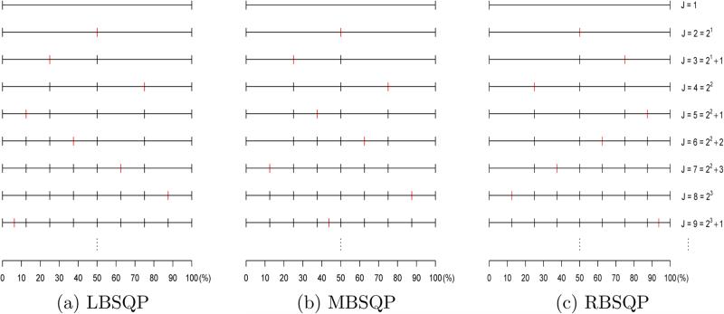
Figure 1 shows how the partition intervals are constructed based on LBSQP, MBSQP, and RBSQP. Notice that when J = 2^K, K = 1, 2, . . . , ESQP, LBSQP, MBSQP, and RBSQP yield the same partition. LBSQP, MBSQP, and RBSQP are desirable when there are more events at the beginning, in the middle, and at the end of the follow-up period, respectively. Another advantage of LBSQP, MBSQP, and RBSQP is that the resulting partitions are nested and, hence, the log-likelihood of the joint model increases in J when the longitudinal component remains fixed.

Figure 1.

An illustration of three bi-sectional partition methods.

2.3. The joint likelihood

We rewrite (1) as follows:

$${\mathit{y}}_i=W_i{({\theta }_i^{\top },{\gamma }^{\top })}^{\top }+{ϵ}_i,$$

where ${\mathit{y}}_i={(y_i\left(a_{i1}\right),\dots ,y_i\left(a_{i{m}_i}\right))}^{\top }$, $W_i={({(g{\left(a_{ij}\right)}^{\top },{\mathit{x}}_i{\left(a_{ij}\right)}^{\top })}^{\top },j=1,\dots ,m_i)}^{\top }$, and ${ϵ}_i={({ϵ}_i\left(a_{i1}\right),\dots ,{ϵ}_i\left(a_{i{m}_i}\right))}^{\top }\sim N(0,{\sigma }^2{I}_{m_i})$. The complete-data likelihood function of the longitudinal measures for the ith subject is given by

$$L(\gamma ,{\sigma }^2\mid {\mathit{y}}_i,W_i,{\theta }_i)=\frac{1}{{\left(2\pi {\sigma }^2\right)}^{\frac{m_i}{2}}}\exp \left\{-\frac{1}{2{\sigma }^2}{({\mathit{y}}_i-W_i{({\theta }_i^{\top },{\gamma }^{\top })}^{\top })}^{\top }({\mathit{y}}_i-W_i{({\theta }_i^{\top },{\gamma }^{\top })}^{\top })\right\},$$ (7)

for i = 1, . . . , n. Note that the density of θ_i is given by

$$f({\theta }_i\mid \theta ,\Omega )=\frac{{\mid \Omega \mid }^{-\frac{1}{2}}}{{\left(2\pi \right)}^{\frac{q+1}{2}}}\exp \left\{-\frac{1}{2}{({\theta }_i-\theta )}^{\top }{\Omega }^{-1}({\theta }_i-\theta )\right\}.$$ (8)

Let φ = (λ, β, α, γ, σ², θ, Ω). Using (2) (or (3)), (7), and (8), the observed-data likelihood function for (y_i, t_i, δ_i) for the ith subject is given by

$$L(\phi \mid {\mathit{y}}_i,t_i,{\delta }_i,{\mathit{z}}_i,W_i)=\int L(\lambda ,\beta ,\alpha \mid t_i,{\delta }_i,{\mathit{z}}_i,{\theta }_i,\mathit{g})L(\gamma ,{\sigma }^2\mid {\mathit{y}}_i,W_i,{\theta }_i)f({\theta }_i\mid \theta ,\Omega )d{\theta }_i,$$ (9)

where the complete-data likelihood function for the survival component is written as

$$L(\lambda ,\beta ,\alpha \mid t_i,{\delta }_i,{\mathit{z}}_i,{\theta }_i,\mathit{g})={\left[\lambda (t_i\mid {\lambda }_0,\beta ,\alpha ,{\theta }_i,\mathit{g}\left(t_i\right),{\mathit{z}}_i)\right]}^{{\delta }_i}\times \exp \left\{-{\int }_0^{t_i}\lambda (u\mid {\lambda }_0,\beta ,\alpha ,{\theta }_i,\mathit{g}\left(u\right),{\mathit{z}}_i)du\right\},$$ (10)

for i = 1, . . . , n. In (2) (or (3)), when β = 0 (or β = 0), the hazard function reduces to λ(t|λ₀, α, z_i) = λ₀(t) exp(${\alpha }^{\top }{\mathit{z}}_i$). In this case, we fit the survival data alone and the likelihood function in (10) for the ith subject reduces to

$$L_0(\lambda ,\alpha \mid t_i,{\delta }_i,{\mathit{z}}_i)={\left\{{\lambda }_0\left(t_i\right)\exp \left({\alpha }^{\top }{\mathit{z}}_i\right)\right\}}^{{\delta }_i}\exp \left[-\exp \left({\alpha }^{\top }{\mathit{z}}_i\right)\left\{{\int }_0^{t_i}{\lambda }_0\left(u\right)du\right\}\right].$$ (11)

Letting D_obs = {(y_i, t_i, δ_i, x_i, z_i), i = 1, . . . , n} denote the observed data, the joint likelihood for all subjects is given by

$$L(\phi \mid \mathit{g},D_{\mathrm{obs}})=\prod _{i=1}^{n}L(\phi \mid {\mathit{y}}_i,t_i,{\delta }_i,{\mathit{z}}_i,W_i).$$ (12)

2.4. AIC (BIC) decomposition and ΔAIC (ΔBIC)

Write φ₁ = (γ, σ², θ, Ω) and φ₂ = (λ, β, α). Let f(θ_i|y_i, W_i, φ₁) be the conditional density of the random effects θ_i given y_i, and also let L(φ₁|y_i, W_i) = ∫L(γ, σ²|y_i, W_i, θ_i)f(θ_i|θ, Ω)dθ_i, which is the likelihood function corresponding to the marginal distribution of y_i. Following Zhang et al. (2014), the joint likelihood given in (12) can be decomposed as

$$L(\phi \mid \mathit{g},D_{\mathrm{obs}})=L_{\mathrm{Long}}({\phi }_1\mid \mathit{g},D_{\mathrm{obs}})L_{\mathrm{Surv}\mid \mathrm{Long}}({\phi }_2\mid \mathit{g},{\phi }_1,D_{\mathrm{obs}}),$$ (13)

where $L_{\mathrm{Long}}({\phi }_1\mid \mathit{g},D_{\mathrm{obs}})={\prod }_{i=1}^{n}L({\phi }_1\mid {\mathit{y}}_i,W_i)$ and $L_{\mathrm{Surv}\mid \mathrm{Long}}({\phi }_2\mid \mathit{g},{\phi }_1,D_{\mathrm{obs}})={\prod }_{i=1}^n\int L({\phi }_2\mid t_i,{\delta }_i,{\mathit{z}}_i,{\theta }_i,\mathit{g})f({\theta }_i\mid {\mathit{y}}_i,W_i,{\phi }_1)d{\theta }_i$. Using (13), the decomposition of the total Akaike Information Criterion (AIC) (Akaike 1973) developed in Zhang et al. (2014) is given as

$$\mathrm{AIC}={\mathrm{AIC}}_{\mathrm{Long}}+{\mathrm{AIC}}_{\mathrm{Surv}\mid \mathrm{Long}},$$

where $\mathrm{AIC}=-2\log L(\widehat{\phi }\mid \mathit{g},D_{\mathrm{obs}})+2\dim \left(\phi \right)$, ${\mathrm{AIC}}_{\mathrm{Long}}=-2\log L_{\mathrm{Long}}({\widehat{\phi }}_1\mid \mathit{g},D_{\mathrm{obs}})+2\dim \left({\phi }_1\right)$, ${\mathrm{AIC}}_{\mathrm{Surv}\mid \mathrm{Long}}=-2\log L_{\mathrm{Surv}\mid \mathrm{Long}}({\widehat{\phi }}_2\mid \mathit{g},{\widehat{\phi }}_1,D_{\mathrm{obs}})+2\dim \left({\phi }_2\right)$, and $\widehat{\phi }$, ${\widehat{\phi }}_1$, and ${\widehat{\phi }}_2$ are the maximum likelihood estimates (MLEs) of φ, φ₁ and φ₂. Similarly, the total Bayesian Information Criterion (BIC) (Schwarz 1978) for the joint model can be decomposed into

$$\mathrm{BIC}={\mathrm{BIC}}_{\mathrm{Long}}+{\mathrm{BIC}}_{\mathrm{Surv}\mid \mathrm{Long}},$$

where BIC = AIC+dim(θ)(log n-2), BIC_Long = AIC_Long+dim(φ₁)(log n−2), BIC_Surv|Long = AIC_Surv|Long + dim(φ₂)(log n−2). Using the decompositions of AIC and BIC, Zhang et al. (2014) proposed two new model assessment criteria given by

$$\begin{array}{cc}\hfill \Delta \mathrm{AIC}=& {\mathrm{AIC}}_{\mathrm{Surv},0}-{\mathrm{AIC}}_{\mathrm{Surv}\mid \mathrm{Long}},\hfill \\ \hfill \Delta \mathrm{BIC}=& {\mathrm{BIC}}_{\mathrm{Surv},0}-{\mathrm{BIC}}_{\mathrm{Surv}\mid \mathrm{Long}},\hfill \end{array}$$

where

$$\begin{array}{cc}\hfill {\mathrm{AIC}}_{\mathrm{Surv},0}=& -2{\sum }_{i=1}^n\log L_0(\widehat{\lambda },\widehat{\alpha }\mid t_i,{\delta }_i,{\mathit{z}}_i)+2\dim (\lambda ,\alpha ),\hfill \\ \hfill {\mathrm{BIC}}_{\mathrm{Surv},0}=& -2{\sum }_{i=1}^n\log L_0(\widehat{\lambda },\widehat{\alpha }\mid t_i,{\delta }_i,{\mathit{z}}_i)+\dim (\lambda ,\alpha )\log n,\hfill \end{array}$$

and L₀(λ, α|t_i, δ_i, z_i) is defined by (11). The ΔAIC or ΔBIC measure the gain of the fit in the survival component due to the longitudinal data with a penalty for the additional parameters in the survival component of the joint model. The model with a large value of ΔAIC (ΔBIC) is more preferred.

3. The SAS macro JMFit

3.1. Design

The SAS macro JMFit has been developed to assess model fit in joint models of longitudinal and survival data. In fact, it can fit five models, including the two types of joint models with linear and quadratic trajectories, as well as the time-varying covariates model. The macro JMFit consists of five submacros, SPM1L, SPM1Q, SPM2L, SPM2Q, and TVC, corresponding to the five models, respectively. The MODEL argument of JMFit specifies one of the following five models to be fitted:

• SPM1L: SPM1 with Linear trajectory. The hazard function has the form

  $$\lambda (t\mid {\lambda }_0,\alpha ,\beta ,{\theta }_i,\mathit{g}\left(t\right),{\mathit{z}}_i)={\lambda }_0\left(t\right)\exp \{\beta ({\theta }_{0i}+{\theta }_{1i}t)+{\alpha }^{\top }{\mathit{z}}_i\}.$$
• SPM1Q: SPM1 with Quadratic trajectory. The hazard function has the form

  $$\lambda (t\mid {\lambda }_0,\alpha ,\beta ,{\theta }_i,\mathit{g}\left(t\right),{\mathit{z}}_i)={\lambda }_0\left(t\right)\exp \{\beta ({\theta }_{0i}+{\theta }_{1i}t+{\theta }_{2i}{t}^2)+{\alpha }^{\top }{\mathit{z}}_i\}.$$
• SPM2L: SPM2 with Linear trajectory. The hazard function has the form

  $$\lambda (t\mid {\lambda }_0,\alpha ,\beta ,{\theta }_i,\mathit{g}\left(t\right),{\mathit{z}}_i)={\lambda }_0\left(t\right)\exp \{{\beta }_1{\theta }_{0i}+{\beta }_2{\theta }_{1i}+{\alpha }^{\top }{\mathit{z}}_i\},$$

  where θ_0i and θ_1i are subject-level random intercept and random slope.
• SPM2Q: SPM2 with Quadratic trajectory. The hazard function has the form

  $$\lambda (t\mid {\lambda }_0,\alpha ,\beta ,{\theta }_i,\mathit{g}\left(t\right),{\mathit{z}}_i)={\lambda }_0\left(t\right)\exp \{{\beta }_1{\theta }_{0i}+{\beta }_2{\theta }_{1i}+{\beta }_3{\theta }_{2i}+{\alpha }^{\top }{\mathit{z}}_i\},$$

  where θ_0i, θ_1i, and θ_2i are random effects (i.e., random intercept, random slope, and random quadratic coefficient).
• TVC: Time-Varying Covariates model. The hazard function has the form

  $$\lambda (t\mid {\lambda }_0,\beta ,\alpha ,{\mathit{z}}_i,y_i\left(t\right))={\lambda }_0\left(t\right)\exp \{\beta y_i\left(t\right)+{\alpha }^{\top }{\mathit{z}}_i\},$$

  where y_i(t) = y_i(a_ij) for a_ij ≤ t < a_i,j+1 for j = 1, . . . , m_i, where a_i,mi+1 = ∞. Note that the TVC model is a“non-joint”model, and the use of this model has great potential for bias (Fisher and Lin 1999).

We provide the two versions of SPM1L, SPM1Q, SPM2L, and SPM2Q with the TS argument. If TS is missing or equal to 0, the joint model will be fit; while “TS=1” yields the corresponding two-stage model. Similar to the method in Tsiatis et al. (1995), (i) we first fit the linear mixed model specified in (1) to the longitudinal data alone and then obtain the estimates of θ_i, denoted by ${\widehat{\theta }}_i$; and (ii) we replace θ_i in (2) or (3) with the estimate ${\widehat{\theta }}_i$ at the second stage. The only difference between the joint model and the corresponding two-stage model is that θ_i in (2) or (3) is replaced with the estimate ${\widehat{\theta }}_i$. This two-stage approach may potentially lead to biased and inefficient estimates (Ibrahim et al. 2010).

The number of intervals J (≥ 1) for the piecewise constant baseline hazard function needs to be specified in the NPIECES argument. For the PARTITION argument, “1” represents “ESQP”, “2” represents “LBSQP”, “3” represents “MBSQP”, and “4” represents “RBSQP”.

JMFit automatically produces a rich text file (rtf) including five tables: (i) Number of Subjects; (ii) Fit Statistics; (iii) Survival Parameter Estimates (Survival Alone); (iv) Parameter Estimates; and (v) Hazard Ratios & λ Estimates.

3.2. Implementation details

If the observed longitudinal measures are sparse, the full trajectories of longitudinal measures might not be well estimated. For example, in the case of fitting a quadratic trajectory, the sign of the estimated second-order coefficient could be incorrect if the longitudinal measures were observed only within the first half of the follow-up period, leading to incorrect extrapolation when the observed progression time was far beyond the time of the last observed longitudinal measure.

Let t_max,i = max_1≤jmi{a_ij}. When t > t_max,i, y_i(t) is never observed and no longitudinal data are available to estimate the trajectory ${\theta }_i^{\top }\mathit{g}\left(t\right)$ for t > t_max,i. Under SPM1, the extrapolation of the trajectory ${\theta }_i^{\top }\mathit{g}\left(t\right)$ beyond t_max,i may lead to a survival component of the joint model that fits the survival data poorly. In addition, such an extrapolation also causes a severe convergence problem in the SAS NLMIXED (SAS Institute Inc. 2011b) procedure especially when t_max,i < < t_i for many subjects. To circumvent these issues, for SPM1, we modify the hazard function in (2) as

$$\lambda (t\mid {\lambda }_0,\alpha ,\beta ,{\theta }_i,\mathit{g},{\mathit{z}}_i)={\lambda }_0\left(t\right)\exp \{\beta {\theta }_i^{\top }\mathit{g}(t-{[t-t_{\max ,i}^{\ast }]}_{+})+{\alpha }^{\top }{\mathit{z}}_i\},$$ (14)

or

$$\lambda (t\mid {\lambda }_0,\alpha ,\beta ,{\theta }_i,\mathit{g},{\mathit{z}}_i)={\lambda }_0\left(t\right)\exp \{\beta {\theta }_i^{\top }\mathit{g}(t-{[t-t_{\max ,i}^{\ast }]}_{+})\times \frac{\tau -(t_{\max ,i}^{\ast }+{[t-t_{\max ,i}^{\ast }]}_{+})}{\tau -t_{\max ,i}^{\ast }}+{\alpha }^{\top }{\mathit{z}}_i\},$$ (15)

where ${[t-t_{\max ,i}^{\ast }]}_{+}=\max (t-t_{\max ,i}^{\ast },0)$, $t_{\max ,i}^{\ast }=t_{\max ,i}+w\times \max (t_i-t_{\max ,i},0)$, w(∈[0,1]) is the proportion of max(t_i − t_max,i,0), and τ = max_1≤i≤n{t_i}, which is the last follow-up survival time. If w = 0 (default), t_max,i will be the starting point of the modified extrapolation of the trajectory; while w = 1 implies that the trajectory extends to t_i with no t_max,i adjustment. This modification can also be applied to the TS model corresponding to SPM1L or SPM1Q. There are two arguments called TMAXI and WEIGHT. If TMAXI is missing or equal to 0, no t_max,i adjustment will be applied. If TMAXI=1, the t_max,i adjustment based on hazard function given in (14) will be applied with weight given in the WEIGHT argument, that is, the trajectory will become flat after $t_{\max ,i}^{\ast }$. If TMAXI=2, the t_max,i adjustment based on hazard function given in (15) will be applied with weight given in the WEIGHT argument, that is, starting at $t_{\max ,i}^{\ast }$, the trajectory will linearly go down to 0 at the last follow-up survival time. An “optimal” choice of weight w in conjunction with TMAXI option may be determined by either AIC_Surv|Long or BIC_Surv|Long. The purpose of defining t_max,i is that we create an extrapolation of the longitudinal measures so that the trajectory function can be well estimated. This extrapolation is needed when there are few longitudinal measures at later points. We note here that the t_max,i method corresponds to a “Prediction Carried Forward” approach, which may potentially induce bias in the estimation. We also note that this is not an issue for the SPM2, in which the hazard function is independent of g(t).

The OPTIONS argument allows users to specify options (e.g., integration method, optimization technique, and convergence criteria) that are available in the PROC NLMIXED statement. If OPTIONS is missing, JMFit will use adaptive Gaussian quadrature to approximate the integral of the likelihood over the random effects, perform a quasi-Newton optimization, and apply a relative gradient convergence criterion of 10⁻⁸. All the methods mentioned above are default methods in PROC NLMIXED. The Riemann integral is used to compute the cumulative hazard function for the trajectory models. Each time interval is divided into 200 subintervals.

A big challenge in fitting joint models using the SAS NLMIXED procedure is convergence. Poor initial values may lead to the failure of convergence in NLMIXED. To address this issue, we first fit the longitudinal data alone using the SAS MIXED procedure to obtain the estimates, $\widehat{\gamma }$, ${\widehat{\sigma }}^2$, $\widehat{\theta }$, $\widehat{\Omega }$, ${\widehat{\theta }}_i$, for the parameters in the longitudinal component of the joint model. Using (${\widehat{\theta }}_i$, i = 1, . . . , n) to replace (θ_i, i = 1, . . . , n) in (2) (or (3)), we fit the survival data alone to obtain the estimates, $\widehat{\beta }$, (or $\widehat{\beta }$), $\widehat{\alpha }$, and $\widehat{\lambda }$, for the parameters in the survival component of the joint model. Finally, these estimates are used as the initial values for the joint model.

JMFit does not exclude any longitudinal measures for the joint models. If one wishes to exclude the longitudinal measures observed after the survival time t_i, those longitudinal measures should be pre-excluded in the input longitudinal data for JMFit. “CAUTION: Longitudinal measures are observed after the survival time.” will be given at the end of the output file if there are any longitudinal measures observed after the survival time.

4. Examples

4.1. The EMPHACIS data

To illustrate how JMFit works, we use the data from a multicenter, randomized, single-blind, EMPHACIS lung cancer clinical trial (Evaluation of MTA in Mesothelioma in a Phase III Study with Cisplatin). The study drug was a multi-targeted antifolate (MTA) pemetrexed which was given in combination with cisplatin (the PEM/Cis arm), and the active-treatment comparator was cisplatin alone (the Cis arm). The treatment for both arms was structured as six 21-day cycles of therapy; patients receiving treatment benefit could receive additional cycles based on investigator discretion.

Malignant pleural mesothelioma is a rapidly progressing and highly symptomatic malignancy with a median survival time of 6 to 9 months. Accordingly, patient-reported assessments are important for evaluation of disease progression and patients’ response to therapy. In oncology, the patients’ importance ratings on the magnitude of progression-free survival improvement have been shown to depend on the severity of disease-related symptoms (Bridges et al. 2012). We analyzed the disease-specific patient-reported Lung Cancer Symptom Scales (LCSS) to evaluate the patient-level association of five instrument items, anorexia, cough, dyspnea, fatigue, and pain, with progression-free survival using EMPHACIS trial data.

We consider the same subset of the EMPHACIS data as in Zhang et al. (2014), which consists of 425 patients with at least one post-baseline value of each longitudinal measure and seven binary covariates, including therapy (1=pemetrexed/cisplatin and 0=cisplatin alone), race (1=white and 0=others), gender (1=male and 0=female), age (1=‘≥ 65’ and 0=‘< 65’), Karnofsky (1=‘90-100’ and 0=‘<90’), stage (1=stage I/II and 0=stage III/IV), and bf (1=full vitamin supplementation and 0=other). The detailed description of this study can be found in Zhang et al. (2014). By applying joint models in this study, we compare the longitudinal LCSS symptoms in terms of their contribution to the overall fit of survival data via ΔAIC and ΔBIC, which are computed using JMFit.

Suppose we fit the trajectory model with a linear trajectory and J = 3 for pain. Then we create two data sets named as “lcss_long_pain” and “lcss_surv_pain” for the macro JMFit's LONG and SURV options, respectively. The MODEL option is set to “SPM1L” and TS is set to 0. We assign 1 to TMAXI for t_max,i adjustment with WEIGHT=0. The NPIECES option is set to 3 and the PARTITION option is set to 2 for the LBSQP algorithm.

JMFit is called:

%JMFit(LONG = lcss_long_pain, SURV = lcss_surv_pain, MODEL = SPM1L, TS = 0, TMAXI = 1, WEIGHT = 0, NPIECES = 3, PARTITION = 2);

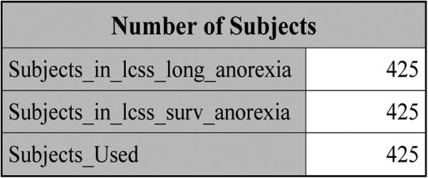
The rtf file “Output for pain under SPM1L with J = 3 (Partition=2).rtf” is generated by JMFit, which lists five tables. Table “Number of Subjects” given in Figure 2 shows that there are 425 patients in data sets lcss_long_pain and lcss_surv_pain, respectively, and 425 subjects are used, implying that the id's of the subjects in these two data sets match.

Figure 2.

The number of subjects for pain.

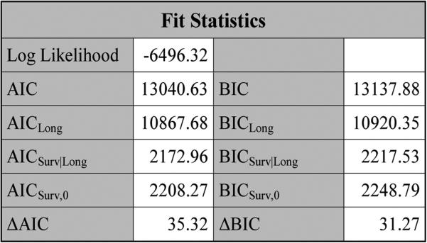
Figure 3 shows the“Fit Statistics”table, which consists of the log likelihood, AIC_Long (BIC_Long), AIC_Surv (BIC_Surv), and ΔAIC (ΔBIC). Inside the JMFit macro, PROC NLMIXED provides the log likelihood, AIC and BIC, and PROC IML (SAS Institute Inc. 2011a) is used to compute AIC_Long and BIC_Long.

Figure 3.

The fit statistics for pain under SPM1L with J = 3 based on LBSQP.

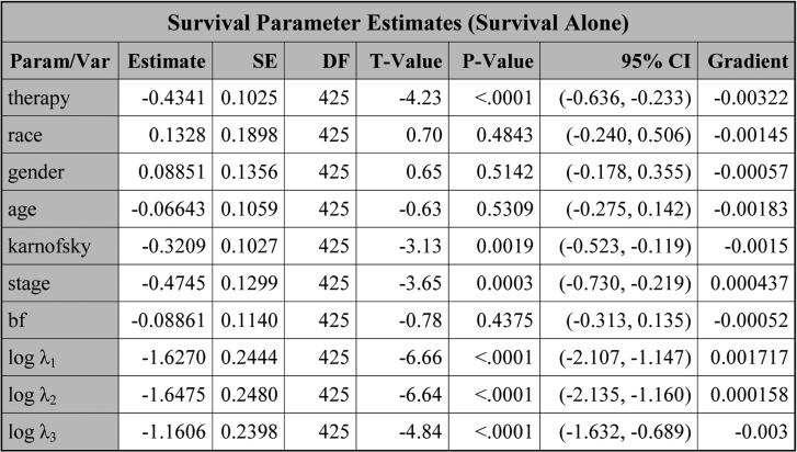
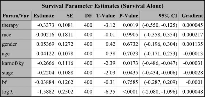
Next, the table, titled “Survival Parameter Estimates (Survival Alone)” shown in Figure 4, is obtained by fitting the survival data alone. For this table, the estimate, the standard error (SE), the degrees of freedom (DF), the t-value, the p-value, and the 95% confidence interval (CI) are all shown for each parameter. In addition, the gradient of the negative log-likelihood function is displayed, which can be used to check convergence of PROC NLMIXED. A small gradient implies better convergence. The largest absolute value of the gradients shown in Figure 4 is 0.00322, indicating good convergence of PROC NLMIXED.

Figure 4.

The estimates of the parameters obtained by (11) with J = 3 based on LBSQP.

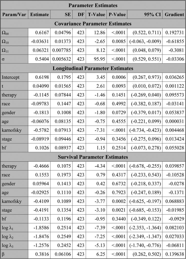
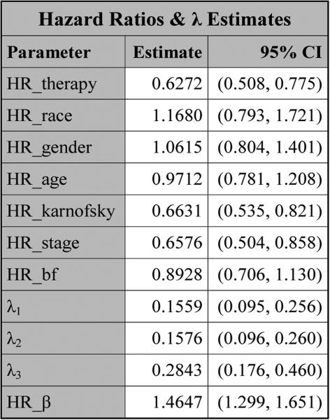
PROC NLMIXED produces the table titled “Parameter Estimates” in Figure 5, which consists of three subtables: “Covariance Parameter Estimates”, “Longitudinal Parameter Estimates”, and “Survival Parameter Estimates”. For each parameter in this table, the estimate, SE, DF, t value, p value, 95% CI, and gradient are all provided. The Subtable “Covariance Parameter Estimates” consists of the estimates of the three lower-triangle elements (Ω₀₀, Ω₁₀, Ω₁₁) of the random-effects covariance matrix as well as the estimate of the standard deviation (σ) for the error term. The estimates of the coefficients of the variables from the longitudinal component are shown in Subtable “Longitudinal Parameter Estimates”. In Subtable “Survival Parameter Estimates”, “Param/Var” lists all the names of the variables as well as the parameters from the survival component. In this subtable, log λ₁, log λ₂, and log λ₃ are the natural logarithms of the piecewise baseline hazards for the three intervals, respectively. The hazard ratios of the covariates and β as well as the estimates of λ are shown in Figure 6. From Figure 5, we see that therapy has p-values of 0.1451 and <.0001 in the longitudinal and survival submodels, respectively, indicating that therapy is not statistically significant at the 0.05 level in the longitudinal submodel and it is highly significant in the survival submodel. Also, from Figure 6, the estimated hazard ratio of therapy in the survival model is 0.6272 with a 95% CI of (0.508, 0.775), implying that the treatment reduces the risk of disease progression by about 37%. From Figure 5, we also see that (i) karnofsky is highly significant in both the longitudinal and survival submodels and (ii) the other significant variables in the survival submodel include the coefficient β corresponding to the linear trajectory and stage. A significant coefficient β indicates that pain is highly associated with disease progression.

Figure 5.

The estimates of the parameters for pain under SPM1L with J = 3 based on LBSQP.

Figure 6.

The hazard ratios and λ estimates for pain under SPM1L with J = 3 based on LBSQP.

From the “Fit Statistics” tables in Figure 3 and Figure 7, we see that pain had the largest values of ΔAIC and ΔBIC and cough had the smallest values of ΔAIC and ΔBIC, which indicate that pain led to the most gain in fitting the PFS data while cough had the least contribution to the fit of the PFS data.

Figure 7.

The fit statistics for anorexia, cough, dyspnea, and fatigue under SPM1L with J = 3 based on LBSQP.

Since ΔAIC = AIC_Surv,0 − AIC_Surv|Long, both AIC_Surv,0 and AIC_Surv|Long change when J changes. Thus, the “best J” based on ΔAIC may not necessarily lead to the best survival submodel or the best joint model. As an illustration, Table 1 shows the values of AIC_Surv|Long and ΔAIC for pain under SPM1L with different partition algorithms and different J's. From Table 1, we see that (i) J = 7 (or J = 6) is the “best” choice according to ΔAIC; (ii) J = 2 is the “best” one based on AIC_Surv|Long; and (iii) the values of AIC_Surv|Long are 2175.29, 2175.29, and 2175.60 for LBSQP, MBSQP, and RBSQP when J = 7, which are much larger than those when J = 2. Since our goal is to fit the joint model to both the longitudinal data and the survival data, it is more appropriate to use AIC_Surv|Long to determine the number of intervals for the piecewise constant baseline hazard function.

Table 1.

AIC_Surv|Long's and ΔAIC's for pain under SPM1L with different partition algorithms and different J's.

J	AICSurv|Long			ΔAIC
	LBSQP	MBSQP	RBSQP	LBSQP	MBSQP	RBSQP
1	2200.94	2200.94	2200.94	24.87	24.87	24.87
2	2170.94	2170.94	2170.94	35.35	35.35	35.35
3	2172.96	2172.96	2172.90	35.32	35.32	34.84
4	2174.91	2174.91	2174.91	34.81	34.81	34.81
5	2176.53	2174.36	2176.84	34.66	35.04	34.68
6	2175.98	2173.66	2176.15	34.89	35.72	35.36
7	2175.29	2175.29	2175.60	35.57	35.57	35.59
8	2177.22	2177.22	2177.22	35.44	35.44	35.44

Table 2 shows the values of AIC_Surv|Long for cough and pain under SPM1L with t_max,i adjustments using different w's. We can see from Table 2 that, among the five values of w, for both t_max,i adjustments, cough and pain have the smallest values of AIC_Surv|Long at w = 0.25 and 0, respectively. For cough, the two t_max,i adjustments result in similar values of AIC_Surv|Long; and for pain, TMAXI=2 slightly outperforms TMAXI=1. In addition, both cough and pain have the largest values of AIC_Surv|Long at w = 1, indicating that the full trajectories were not well estimated.

Table 2.

AIC_Surv|Long's for cough and pain under SPM1L with t_max,i adjustments using different w's.

w	Cough		Pain
	TMAXI=1	TMAXI=2	TMAXI=1	TMAXI=2
0	2200.97	2200.88	2170.94	2168.33
0.25	2200.48	2200.74	2172.84	2171.65
0.5	2201.71	2201.51	2177.09	2175.40
0.75	2204.21	2203.63	2182.34	2180.72
1a	2206.68	2206.68	2186.46	2186.46

^aNo t_max,i adjustment

4.2. A simulated data example

Since we do not have permission to distribute the EMPHACIS dataset used in Section 4.1 publicly, we consider a simulated data example, in which the simulated data can be downloaded directly from the journal's website.

We generated a simulated data set with n = 400 subjects as follows. First, the time points (a_ij's) at which the longitudinal measures were taken were fixed at (0, 21, 42, 63, 84, 105, 126)/30.4375. For each subject, we generated seven binary covariates, (x_i1, . . . , x_i7), independently from Bernoulli distributions with success probabilities (i.e., P(x_ij = 1), j = 1, . . . , 7)) 0.49, 0.92, 0.81, 0.49, 0.38, 0.56, and 0.74, respectively. These proportions were estimated from the EMPHACIS data, corresponding to the covariates treatment, race/ethnicity, gender, age, Karnofsky status, baseline stage of disease, and vitamin supplementation, respectively. Second, we simulated the longitudinal trajectory as

$${\mu }_i\left(a_{ij}\right)=({\theta }_0+{\theta }_{0i})+({\theta }_1+{\theta }_{1i})a_{ij}+\gamma {\mathit{x}}_i,$$

where θ₀ = 0.62, θ₁ = 0.04, $\gamma ={(-0.11,-0.10,-0.18,-0.06,-0.58,-0.09,0.10)}^{\top }$, and ${({\theta }_{0i},{\theta }_{1i})}^{\top }\sim N(0,\left(\begin{array}{cc}\hfill 0.62\hfill & \hfill -0.04\hfill \\ \hfill -0.04\hfill & \hfill 0.06\hfill \end{array}\right))$. Finally, we generated the longitudinal data from a N(μ_i(a_ij), σ²) distribution with σ = 0.54 and $t_i^{\ast }$ as

$$t_i^{\ast }=-\frac{\log (1-U)}{\lambda \exp \{{\beta }_1({\theta }_0+{\theta }_{0i})+{\beta }_2({\theta }_1+{\theta }_{1i})+\alpha {\mathit{x}}_i\}},$$

where $\alpha ={(-0.36,0.15,0.04,-0.003,-0.33,-0.38,-0.07)}^{\top }$, β₁ = 0.26, β₂ = 1.17, λ = exp(−1.67), and U ~ U(0,1). This longitudinal dataset is denoted by D_Long. Note that the values of the parameters were obtained by fitting SPM2L to the EMPHACIS data in which the longitudinal measure corresponds to pain. The censoring time C_i was generated from an exponential distribution with mean 50, and the right-censoring percentage was about 12%. The failure time and censoring indicator were calculated as $t_i=\min \{t_i^{\ast },C_i\}$ and ${\delta }_i=1\{t_i^{\ast }\le C_i\}$, where 1{A} denotes the indicator function such that 1{A} = 1 if A is true and 0 otherwise. This survival dataset is denoted by D_Surv.

We also generated three additional sets of longitudinal data, with longitudinal trajectories simulated from

$${\mu }_{\ell i}\left(a_{ij}\right)=({\theta }_0+{\theta }_{0i}+{\tau }_{\ell 0i})+({\theta }_1+{\theta }_{1i}+{\tau }_{\ell 1i})a_{ij}+\gamma {\mathit{x}}_i,$$

where (i) ${({\tau }_{10i},{\tau }_{11i})}^{\top }\sim N(0,\left(\begin{array}{cc}\hfill {0.1}^2\hfill & \hfill 0\hfill \\ \hfill 0\hfill & \hfill {0.1}^2\hfill \end{array}\right))$; (ii) ${({\tau }_{20i},{\tau }_{21i})}^{\top }\sim N(0,\left(\begin{array}{cc}\hfill {0.5}^2\hfill & \hfill 0\hfill \\ \hfill 0\hfill & \hfill {0.5}^2\hfill \end{array}\right))$; and (iii) ${({\tau }_{30i},{\tau }_{31i})}^{\top }\sim N(0,\left(\begin{array}{cc}\hfill 1\hfill & \hfill 0\hfill \\ \hfill 0\hfill & \hfill 1\hfill \end{array}\right))$. Then the longitudinal data were generated from a N(μ_ℓi(a_ij), σ²) distribution with σ = 0.54 for ℓ = 1, 2, 3. These three additional sets of longitudinal data were coupled with the same survival times as in D_Long + D_Surv to form three additional data sets. These resulting data sets are denoted by D_Long1 + D_Surv, D_Long2 + D_Surv, and D_Long3 + D_Surv. This simulation setting is similar to Simulation III in Zhang et al. (2014) except for the six additional covariates.

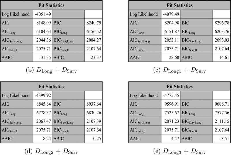
Figure 8 shows the fit statistics for D_Long + D_Surv, D_Long1 + D_Surv, D_Long2 + D_Surv, and D_Long3 + D_Surv, respectively, using JMFit. We see from Figure 8 that D_Long + D_Surv has the largest values of ΔAIC and ΔBIC.

Figure 8.

The fit statistics for D_Long + D_Surv, D_Long1 + D_Surv, D_Long2 + D_Surv, and D_Long3 + D_Surv under SPM2L.

The rest of the output for D_Long + D_Surv are provided in Appendix B. The output for D_Longℓ+D_Surv (ℓ = 1, 2, 3) are omitted here for brevity.

5. Concluding remarks

The JMFit SAS macro fits the joint models for longitudinal and survival data. The piecewise exponential constant hazard model is assumed for the baseline hazard function. The time-axis is partitioned into J intervals, which are constructed by four algorithms, namely, ESQP, LBSQP, MBSQP, and RBSQP. JMFit allows users to specify the number of intervals J and the partition method. Five models, including SPM1L, SPM1Q, SPM2L, SPM2Q, and TVC, are implemented in JMFit. This SAS macro also computes AIC, BIC, ΔAIC, ΔBIC, and the estimates of the parameters in the joint model. The computational time of JMFit depends on which of SPM1L, SPM1Q, SPM2L, SPM2Q, or TVC is chosen and how big the dataset is. For the example given in Section 4.1, it took 42 seconds to fit SPM1L with J = 3 based on LBSQP for pain on a Dell PC with an Intel i5 processor, 3.30 GHz CPU, and 8 GB of memory. On the same PC, it only took 10 to 11 seconds to fit SPM2L to each of the simulated datasets illustrated in Section 4.2.

The JMFit SAS macro provides two versions for SPM1L, SPM1Q, SPM2L, and SPM2Q with the TS argument, with “TS=1” yielding the corresponding two-stage model. Comparing these models with TS missing or equal to 0, for the two-stage models, (i) we first fit (1) to the longitudinal data alone and obtain the estimates of θ_i, denoted by ${\widehat{\theta }}_i$; and (ii) we then use ${\widehat{\theta }}_i$ in (2) and (3). The TS models are also substantially different than the TVC model since the TS models do not require the LOCF assumption.

The current version of the JMFit SAS macro only fits linear and quadratic models for the longitudinal outcome and the piecewise constant baseline hazard function for the survival submodel. In the joint modeling framework, other dependence structures, such as dependence through the derivatives of the trajectory function or interactions with covariates as well as spline approximations to the baseline hazard could be assumed. In addition, other trajectory functions may be more appropriate to model the time effect on the longitudinal outcomes in certain applications. These additional features could be built in the JMFit macro in a future release.

Finally, we note that the EMPHACIS dataset used in this paper is proprietary and cannot be distributed publicly. However, the simulated datasets D_Surv, D_Long, D_Long1, D_Long2, and D_Long3 are available for downloading from the journal website.

A. The macro JMFit

The SAS macro JMFit as well as the five submacros should be stored in a folder named “jmfit”. Then JMFit can be accessed by including the following lines:

filename jmfit “directory of the file JMFit”;
%include jmfit(JMFit.sas);
%JMFit(LONG=, SURV=, MODEL=, TS=, TMAXI=, WEIGHT=, NPIECES=, PARTITION=, OPTIONS=, INITIAL=, OUTPUT=);

Inputs for JMFit

LONG: Data set with the first three columns, SID (subject ID), Y (longitudinal measure), A (time at which Y was taken), and additional columns for covariates (X_L1-X_Lp), where SID, Y, and A should be arranged in the first, second, and third columns, and X_L1, ···, X_Lp should be placed after column 3, which can be enforced in SAS by using the “retain” command. Note that X_L1, ..., X_Lp can be time-dependent or baseline covariates. Required.

SURV: Data set with the first three columns, SID, survival time (T), censoring indicator (delta) (1 = death and 0 = censored), and additional columns for covariates (X_S1-X_Sq), where SID, T, and delta should be arranged in the first, second, and third columns, and X_S1, . . . , X_Sq should be placed after column 3. Required.

MODEL: Model specification. Required. One of

1. SPM1L: Shared Parameter Model 1 with Linear trajectory.

2. SPM1Q: Shared Parameter Model 1 with Quadratic trajectory.

3. SPM2L: Shared Parameter Model 2 with Linear trajectory.

4. SPM2Q: Shared Parameter Model 2 with Quadratic trajectory.

5. TVC: Time-Varying Covariates Model.

TS: Indicates whether to implement the model specified in the MODEL argument or the corresponding two-stage model. If 0 (default), the model specified in the MODEL argument will be fit. If 1, the corresponding two-stage model will be fit instead. It only works for SPM1L, SPM1Q, SPM2L, and SPM2Q.

TMAXI: t_max,i adjustment to the model specified in the MODEL argument. If 0 (default), no t_max,i adjustment will be applied. If 1, the trajectory will become flat after $t_{\max ,i}^{\ast }=t_{\max ,i}+\mathrm{WEIGHT}\times \max (t_i-t_{\max ,i},0)$. If 2, starting at $t_{\max ,i}^{\ast }$, the trajectory will linearly go down to 0 at the last follow-up survival time. It only works for SPM1L and SPM1Q.

WEIGHT: The proportion (∈ [0, 1]) of max(t_i − t_max,i, 0). If 0 (default), the starting point of the modified extrapolation of the trajectory is t_max,i. If 1, the trajectory extends to t_i with no t_max,i adjustment. It only works when TMAXI=1 or TMAXI=2.

NPIECES: Number of intervals J (≥ 1) for the piecewise constant baseline hazard function.

Required.

PARTITION: Algorithm for constructing the partition of the time axis. Required. One of

• (i)1: Equally-Spaced Quantile Partition (ESQP).
• (ii)2: Left Bi-Sectional Quantile Partition (LBSQP).
• (iii)3: Middle Bi-Sectional Quantile Partition (MBSQP).
• (iv)4: Right Bi-Sectional Quantile Partition (RBSQP).

OPTIONS: Allows users to specify options that are available in the PROC NLMIXED statement. For example, “OPTIONS=%str(QPOINTS=5 TECH=CONGRA ABSGCONV=0.0001)” specifies Gaussian quadrature with five quadrature points for approximating the integral of the likelihood over the random effects, the conjugate-gradient optimization, and an absolute gradient convergence criterion of 0.0001.

INITIAL: Allows users to set their own initial values. JMFit will automatically generate the starting values for the model parameters and these initial values will be stored in the data set “_initial”. Since the order of the parameters is very important when calculating AIC_Long and BIC_Long, users are recommended to change the initial values in “_initial” and then rename “_initial”.

OUTPUT: Name of the output rich text file (rtf). One can also specify the directory in which the file will be put. For example, the output file named “myoutput” will be stored in “C:\ . . . ” by “%JMFit(..., OUTPUT = C: \. . . \myoutput);” If OUTPUT is not specified, the file will be indexed by the name of Y from LONG and the model's name.

• Note 1: (i) The name of the SID variable in LONG should be the same as that of the SID variable in SURV; (ii) A and T should be in the same unit of time (month preferred); (iii) the categorical covariates must be coded as dummy variables; and (iv) the SAS macro allows for any numbers of covariates for both components of the joint model and the covariates for the longitudinal component can be totally different from those for the survival component.

• Note 2: (i) “ERROR: Not enough memory to generate code.” This might occur if J is too big; (ii) a too long path for the OUTPUT may lead to an error; (iii) the macro is assuming “options validvarname=v7;” for valid variable names that can be processed in SAS; and (iv) the calculations of AIC_Long and BIC_Long require the IML Procedure.

• Note 3: No missing values are allowed in both data sets.

Output for JMFit

The macro automatically produces an rtf file indexed by the name of Y from LONG and the model's name. The rtf file includes five tables: (i) Number of Subjects; (ii) Fit Statistics; (iii) Survival Parameter Estimates (Survival Alone); (iv) Parameter Estimates; and (v) Hazard Ratios & λ Estimates.

Note: The construction of the Parameter Estimates table is different for each model. For SPM1L, SPM1Q, SPM2L, and SPM2Q, it consists of three subtables: “Covariance Parameter Estimates”, “Longitudinal Parameter Estimates”, and“Survival Parameter Estimates”; for the TS model corresponding to SPM1L, SPM1Q, SPM2L, or SPM2Q, there are two tables: “Longitudinal Parameter Estimates (Stage I)” and “Survival Parameter Estimates (Stage II)”; and for the TVC model, there is only one table named“Parameter Estimates”.

B. Output for the simulated data D_Long + D_Surv under SPM2L

Figure 9.

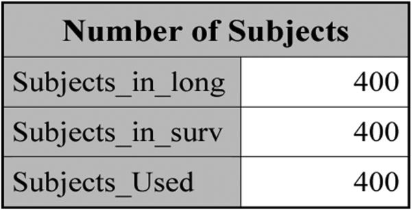
The number of subjects for D_Long + D_Surv.

Figure 10.

The estimates of the parameters obtained by fitting the survival data alone for D_Long + D_Surv.

Figure 11.

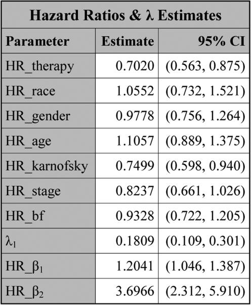
The hazard ratios and λ estimates for D_Long + D_Surv under SPM2L.

Figure 12.

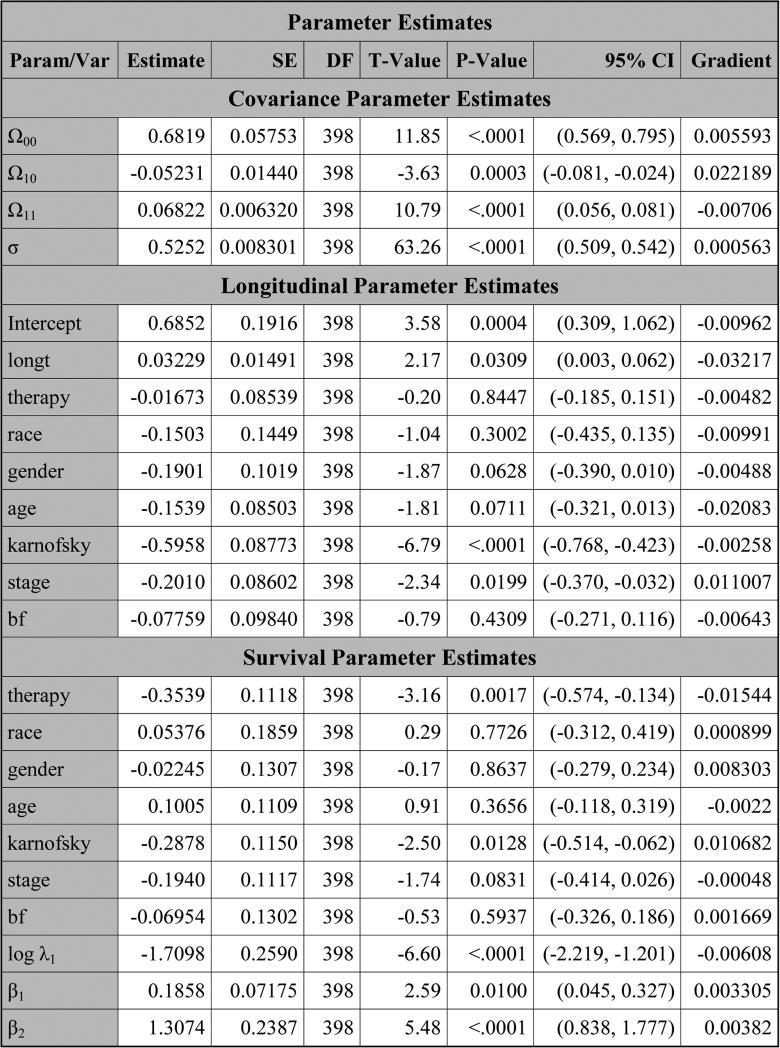
The estimates of the parameters for D_Long + D_Surv under SPM2L.

References

- Akaike H. Information Theory and an Extension of the Maximum Likelihood Principle. In: Petrov BN, Csaki F, editors. Proceedings of the Second International Symposium on Information Theory. Akademiai Kiado; Budapest: 1973. pp. 267–281. [Google Scholar]
- Bridges JFP, Mohamed AF, Finnern HW, Woehl A, Hauber AB. Patients’ Preferences for Treatment Outcomes for Advanced Non-Small Cell Lung Cancer: A Conjoint Analysis. Lung Cancer. 2012;77:224–231. doi: 10.1016/j.lungcan.2012.01.016. [DOI] [PubMed] [Google Scholar]
- Crowther MJ. STJM: Stata Module to Fit Shared Parameter Joint Models of Longitudinal and Survival Data. 2012 URL http://econpapers.repec.org/software/bocbocode/s457502.htm/
- Crowther MJ, Abrams KR, Lambert P. Joint Modeling of Longitudinal and Survival Data. The Stata Journal. 2013;13:165–184. [Google Scholar]
- Fisher LD, Lin D. Time-Dependent Covariates in the Cox Proportional-Hazards Regression Model. Annual Review of Public Health. 1999;20:145–157. doi: 10.1146/annurev.publhealth.20.1.145. [DOI] [PubMed] [Google Scholar]
- Ibrahim JG, Chen MH, Sinha D. Bayesian Survival Analysis. Springer-Verlag; New York: 2001. [Google Scholar]
- Ibrahim JG, Chu H, Chen LM. Basic Concepts and Methods for Joint Models of Longitudinal and Survival Data. Journal of Clinical Oncology. 2010;28:2796–2801. doi: 10.1200/JCO.2009.25.0654. [DOI] [PMC free article] [PubMed] [Google Scholar]
- Philipson P, Sousa I, Diggle P, Williamson P, Kolamunnage-Dona R, Henderson R. joineR: Joint Modelling of Repeated Measurements and Time-to-Event Data. R package version 1.0-3. 2012 URL http://cran.r-project.org/web/packages/joineR/index.html.
- SAS Institute Inc . SAS/IML Software, Version 9.3. Cary, NC: 2011a. URL http://www.sas.com/ [Google Scholar]
- SAS Institute Inc . SAS/STAT Software, Version 9.3. Cary, NC: 2011b. URL http://www.sas.com/ [Google Scholar]
- Proust-Lima C, Philipps V, Diakite A, Liquet B. lcmm: Estimation of Extended Mixed Models Using Latent Classes and Latent Processes. R package version 1.6-4. 2014 URL http://cran.r-project.org/web/packages/lcmm/index.html.
- Rizopoulos D. JM: An R Package for the Joint Modelling of Longitudinal and Time-to-Event Data. Journal of Statistical Software. 2010;35:1–33. [Google Scholar]
- Rizopoulos D. JM: Joint Modeling of Longitudinal and Survival Data. R package version 1.1-0. 2012 URL http://rwiki.sciviews.org/doku.php?id=packages:cran:jm.
- Rizopoulos D. JMbayes: Joint Modeling of Longitudinal and Time-to-Event Data under a Bayesian Approach. R package version 0.5-3. 2014 URL http://cran.r-project.org/web/packages/JMbayes/index.html.
- Schwarz G. Estimating the Dimension of a Model. The Annals of Statistics. 1978;6:461–464. [Google Scholar]
- Tsiatis AA, DeGruttola V, Wulfsohn MS. Modelling the Relationship of Survival to Longitudinal Data Measured with Error. Applications to Survival and CD4 Counts in Patients with AIDS. Journal of the American Statistical Association. 1995;90:27–37. [Google Scholar]
- Zhang D, Chen MH, Ibrahim JG, Boye ME, Wang P, Shen W. Assessing Model Fit in Joint Models of Longitudinal and Survival Data with Applications to Cancer Clinical Trials. Statistics in Medicine. 2014 doi: 10.1002/sim.6269. doi:10.1002/sim.6269. [DOI] [PMC free article] [PubMed] [Google Scholar]