

Abstract
Hydrophobic hydration plays a key role in a vast variety of biological processes, ranging from the formation of cells to protein folding and ligand binding. Hydrophobicity scales simplify the complex process of hydration by assigning a value describing the averaged hydrophobic character to each amino acid. Previously published scales were not able to calculate the enthalpic and entropic contributions to the hydrophobicity directly. We present a new method, based on Molecular Dynamics simulations and Grid Inhomogeneous Solvation Theory, that calculates hydrophobicity from enthalpic and entropic contributions. Instead of deriving these quantities from the temperature dependence of the free energy of hydration or as residual of the free energy and the enthalpy, we directly obtain these values from the phase space occupied by water molecules. Additionally, our method is able to identify regions with specific enthalpic and entropic properties, allowing to identify so-called “unhappy water” molecules, which are characterized by weak enthalpic interactions and unfavorable entropic constraints.
Introduction
Hydrophobic interactions are among the most important driving forces in nature, e.g. responsible for the separation of water and oil, the function of detergents, distribution of minerals in the earth’s crust, and many more.1,2 In biology, they determine the structure of proteins and cells as well as the self-assembly of membranes.3,4 Furthermore, the hydrophobic effect plays a key role in ligand binding processes and needs to be accounted for in drug design.5,6 In all these systems, apolar groups tend to cluster together in a polar liquid, like water, to minimize the surface between groups of different polarity.7 Investigation of the hydrophobic character of compounds is a complex research field because size, shape, and positions of chemical groups have to be taken into account for a detailed understanding.8,9
A common way to simplify the solvation problem for biomolecules is the use of hydrophobicity scales. These scales assign a value to each amino acid, which describes the relative averaged hydrophobic character in comparison to the other amino acids. A vast variety of different scales are discussed in the literature, which are based on various theoretical and experimental methods.10−13 Hydrophobicity scales have been widely used for the prediction of protein secondary structures, membrane regions, antigenic sites, and interior-exterior regions.10,14 However, they have two major drawbacks: first, they describe the averaged hydrophobic character over the whole amino acid and a spatial resolution is not available. The hydrophobicity of a binding pocket may not be uniform, and, therefore, the identification of regions which are especially hydrophobic or hydrophilic is of interest. The displacement of water molecules from these areas into the bulk can lead to significant changes in the free energy of binding. Second, none of the reported methods can directly measure entropic contributions to the hydration process. Methods based on the distribution coefficient – or the free energy of transfer – between two different phases cannot evaluate the entropic contribution directly but only estimate it from the temperature dependence of the free energy or via the difference of the free energy and the enthalpy.15,16 Thus, it is not possible to draw a conclusion about the water dynamics, and a detailed understanding of the entropic effects cannot be reached. This is one of the reasons why – compared to the structural and enthalpic effects of hydration – little is known about the water dynamics and entropic effects around a solute.17
Although many different models are published,18−23 trying to explain the entropic contributions to hydration, especially the extent of the deceleration and entropy gain in the proximity of a solute, is still discussed controversially. Dating back to 1945, Frank and Evans18 were the first to address this issue when they proposed their visionary “Iceberg” model. They suggested that a water cage is formed around a solute in a similar way as it is found in ice or clathrates. This is achieved by orientating the hydrogen bonds tangentially to the solute surface, resulting in a slower reorientation and translation than in bulk.19,24 These restrictions reduce the phase space, which water molecules can occupy in the hydration shells of the solute, resulting in a decrease of entropy.9,17 Due to the strong enthalpic interactions between the solvent and the solute the movement of water molecules around hydrophilic groups is even more restricted. This effect is also known as entropy-enthalpy-compensation and has its origin in the strong electrostatic interactions of polar groups and a polar solvent.25 The increased ordering around solvated molecules can be understood as an entropy penalty for the enthalpic interaction. Although the kinetics of water molecules are slowed down comparable to water in the ice phase, it still remains in a liquidlike structure.26−28 Galamba proposed that these water molecules behave similarly to water molecules at lower temperatures.29 Water dynamics in the solvation process were also analyzed by a variety of experimental techniques and simulations, leading to different interpretations of the results.30−69 The entropic behavior of water molecules in response to different nonpolar, polar, and charged solutes is still elusive, making it one of the remarkable varieties of water properties, which are not completely understood.
Therefore, computer simulations can help to obtain a detailed molecular description of solvation and explain the different thermodynamic contributions to this process. An atomistic understanding is crucial to comprehend the process of solvation in detail. Different theoretical strategies have been reported to describe the effect of hydrophobic interactions, especially in biomolecules. Most of the earlier studies are based on simplified solvent models, described by linear response theory, causing errors in calculations of dipolar solvents.35 More recent reports investigated the size effect of a spherical symmetric solute, the influence of chain lengths on hydrophobicity, and the temperature behavior of hydration properties.36,37 Huggins and Payne reported the hydration free energies for six small molecules calculated with inhomogeneous solvation theory (IST) and thermodynamic integration (TI). Their study revealed a good agreement between the two methods, but the entropy term (−TΔS) in IST calculations is generally overestimated.38 Furthermore, the role of the hydrophobic effect for the behavior of proteins and amino acids has been explored by investigating thermodynamic properties around a set of noncharged amino acids side chain analogues using thermodynamic integration and hydrogen bond analysis.39−41 However, further work showed that the backbone of the amino acid side chain has a significant influence on the thermodynamic properties of the side chain solvation. Therefore, hydrophobic properties of side chain analogues may differ from those of amino acids, including the backbone atoms.15,42,43
In this study, the hydrophobicity of the 20 canonical amino acids is investigated. Amino acid models include the backbone, which has shown to be essential to obtain reliable results. Molecular Dynamics simulations and grid inhomogeneous solvation theory (GIST) are used to simulate and analyze the solvation of amino acids at an atomistic scale. Based on the interaction free energy of amino acids with water molecules we propose a method to calculate hydrophobicity, which allows a direct distinction between enthalpic and entropic contributions. Entropic contributions are obtained directly from the phase space, which water can occupy. We also investigate the spatial resolution of the solvation process, which our method can provide. Dissection of spatially resolved entropic and enthalpic contributions provides additional insight into the entropic behavior of water molecules around a solute.
Computational Methods
Grid Inhomogeneous Solvation Theory
In this section a very brief introduction to the concept of Grid Inhomogeneous Solvation Theory (GIST) developed by Gilson and co-workers is provided. For a more detailed description of GIST we refer to their papers.44,45
Most general, the free energy of solvation for a molecule ΔGSolv can be written as
| 1 |
It is defined as the integral over the free energy of the molecule ΔGSolv(q) with the solute being constrained to configuration q times the probability p(q) to find the solute in state q. For GIST calculations, the molecule is restricted to one single conformation. The impact of other conformations can be accounted for by using multiple GIST calculations on all relevant conformations. In the following, for the sake of simplicity, it is assumed that only one relevant conformation exists. The theory can simply be extended to multiple configurations using eq 1.
The free energy of solvation ΔGSolv can be written as the difference between the solvation enthalpy ΔESolv and the solvation entropy ΔSSolv multiplied by the temperature T:
| 2 |
The underlying idea behind inhomogeneous solvation theory is to transform integrals over molecular coordinates to integrals over distribution functions (one-body, two-body, three-body, correlation functions etc.). Based on these functions it is possible to approximate thermodynamic quantities. GIST uses a grid to discretize the analytical expressions usually used in inhomogeneous solvation theory. Thermodynamic quantities are calculated as discrete values from the stored trajectory frames at every grid point. The solvation enthalpy ΔESolv consists of two terms as shown in eq 3, the interaction between the solvent and the solute, from now on denoted as solute-water interaction ΔESW, and the changes in the enthalpic interaction between the solvent molecules due to the presence of the solute in contrast to the unperturbed water, summarized in ΔEWW.
| 3 |
Both terms are calculated for each voxel of the grid. The solute-water interaction is the interaction of all water molecules in the voxel with the solute molecule, averaged over the complete simulation time. The energy calculation is based on the used simulation force field. In our case this is the AMBER force field46 and an TIPXP solvent model (X = 3,4,5). Similarly, the water–water enthalpy captures the interaction of all water molecules in the voxel with all other water molecules in the simulated system, again averaged over the whole simulation time. The solvation entropy ΔSSolv is approximated by two computational affordable and intuitive terms: the translational ΔStrans and the orientational part ΔSorient of the entropy.
| 4 |
The water–water correlations are neglected, hence, the integrals depend only on the coordinates of one water molecule. The contributions of higher order terms are considered to be small compared to the first order term and slow down the convergence so that longer simulation times would be required.47
The distribution of the water molecules can be written as a function of the position of the oxygen atom of the water molecule in three-dimensional space r and of the orientation of the water molecule ω. Therefore, the water distribution gSW(r,ω) is dependent on two variables. This function can be rewritten as a function gSW(r) only depending on the position r of the water molecule and an orientational part depending solely on ω, with a fixed r value as condition gSW(ω|r), shown in eq 5.
| 5 |
This spliced function can be used to split the approximated entropy into an orientational and a translational term. The translational part depends only on the position of the water molecule in space and can be calculated according to eq 6
| 6 |
where ρ is the number density of the water model. A uniform distribution with the same density of water molecules in every voxel (gSW(r) = 1 for all voxels) is characteristic for a low ordered system with high entropy. If the system shows differences in the density the entropy gets lower (more ordered water structure, gSW(r) ≠ 1). Pure water without any solute has a uniform distribution and serves as reference state. For this reason, all results can be compared to this state. Presented thermodynamic values denote the difference between the observed state and the unperturbed water reference.
The orientational part of the entropy is described by eqs 7 and 8 and describes whether the water molecules in a voxel are found in a similar orientation ω
| 7 |
| 8 |
where gSW(r) is the translational part of the water density, K is a normalization factor, and gSW(ω|r) is the part of the water density distribution gSW(r,ω) depending only on the orientation ω of the water molecule. It is assumed that the orientation of the water is independent of the water position in the voxel. Again, a uniform distribution accounts for low ordering and a high entropy value. In unperturbed/pure water, the individual molecules do not have a preferred orientation but show random orientation.
To summarize, ΔGSolv gives a value for the change in the free energy when the molecule is transferred from the vacuum with no interaction partner to the liquid phase. The free energy consists of the solute-water enthalpy and the water–water enthalpy, as well as the translational and the orientational entropy of the water molecules. In contrast to previously published theoretical studies, the described method calculates the entropy directly from the phase space that water molecules occupy. Other methods like TI usually calculate the entropy as the difference between free energy and enthalpy or use multiple simulations at different temperatures to calculate the entropy due to the temperature dependence of the free energy.
Simulation Details
All 20 canonical amino acids were capped with an N-terminal acetyl and a C-terminal amide group (ACE-X-NME) and solvated in an octahedral box using the AmberTools package.46 The minimum distance between the box edge and the protein was set to 12 Å, resulting in a system with approximately 2000 water molecules. As the water model is known to heavily influence the obtained thermodynamic properties, several water models were used in this study to investigate their impact on hydrophobicity.48 We used the three most common water models in the AMBER package TIP3P,49 TIP4P,49 and TIP5P.50
Arginine and lysine were simulated with a positive charge; glutamate and aspartate were assigned a negative charge. Histidine was simulated as positive and neutral species. For the neutral species we took the average of the two possible states. The backbone was constrained in the same conformation for all amino acids to eliminate the effects of backbone conformations. We choose the most abundant backbone conformation of an unrestrained alanine simulation as our reference geometry. The side chains were set up randomly and allowed to move during the equilibration phase and were restrained during the production run as it is required for the GIST analysis.
Equilibration of the systems was performed according to the established protocol of Wallnöfer et al.51 After equilibration every capped amino acid was simulated in a NPT ensemble for 200 ns. Langevin thermostat was used to keep the temperature at 300 K. The pressure of 1 bar was kept by using an isotropic implementation of the Berendsen barostat. The time step was set to 2 fs, and coordinates were saved every 10 ps.
Simulation time and duration between two snapshots were chosen after a convergence analysis of the thermodynamic properties obtained with GIST. Even though for alanine a 50 ns simulation with 5000 snapshots is sufficient for the GIST analysis, to ensure the convergence for all amino acids the simulation time was extended to 200 ns with 10 000 simulation snapshots. These values are also far beyond the limits suggested in the Amber14 manual.46 The grid spacing was set to 0.5 Å. All grid points within 4 Å of the solute were used to determine the thermodynamic properties of the hydrating water molecules (density-weighted integration). A higher cutoff increases the signal-to-noise ratio and is therefore not practicable. To increase the accuracy of the results and estimate the error correctly the calculations were repeated three times with different initial coordinates for the side chains. The backbone was always restrained to the same conformation. The standard deviation of three runs and the mean were calculated.
Results
Molecular Dynamics simulations of amino acids surrounded by water molecules were performed to calculate thermodynamic properties of the solvation process of these amino acids on a grid around the solute. The results for the free energy, the total enthalpy, and the overall entropy are reported in Table 1 for the three different water models TIP3P, TIP4P, and TIP5P. In the Supporting Information, tables including further decomposition of the enthalpy in solute-water and water–water enthalpy are provided. Additionally, the values for the orientational and translational part of the entropy are summarized for all amino acids and water models.
Table 1. Thermodynamic Quantities: Free Energy, Enthalpy, and Entropy for All 20 Amino Acids Calculated with the Amber Force Field and Three Water Modelsa.
| water
model |
|||||||||
|---|---|---|---|---|---|---|---|---|---|
| TIP3P |
TIP4P |
TIP5P |
|||||||
| amino acid | ΔH | –TΔS | ΔG | ΔH | –TΔS | ΔG | ΔH | –TΔS | ΔG |
| ASP(−) | –80.5 ± 0.3 | 26.4 ± 0.0 | –54.2 ± 0.3 | –82.8 ± 4.2 | 29.2 ± 0.1 | –53.5 ± 4.1 | –67.0 ± 2.8 | 25.3 ± 0.1 | –41.7 ± 2.7 |
| GLU(−) | –78.3 ± 1.9 | 27.7 ± 0.2 | –50.6 ± 1.7 | –85.9 ± 1.3 | 30.6 ± 0.1 | –55.2 ± 1.1 | –68.6 ± 1.6 | 26.5 ± 0.1 | –42.1 ± 1.6 |
| LYS(+) | –66.1 ± 2.5 | 22.8 ± 0.7 | –43.4 ± 1.9 | –63.0 ± 0.9 | 23.5 ± 0.2 | –39.5 ± 0.7 | –69.0 ± 0.6 | 25.6 ± 0.4 | –43.3 ± 0.3 |
| ARG(+) | –64.7 ± 2.1 | 24.1 ± 0.5 | –40.7 ± 1.6 | –62.8 ± 0.5 | 24.5 ± 0.3 | –38.3 ± 0.4 | –72.1 ± 1.9 | 29.4 ± 0.6 | –42.8 ± 1.5 |
| HIS(+) | –57.7 ± 1.6 | 21.5 ± 0.3 | –36.2 ± 1.3 | –56.0 ± 0.7 | 22.5 ± 0.2 | –33.5 ± 0.7 | –60.2 ± 2.8 | 24.3 ± 0.5 | –35.9 ± 2.3 |
| GLN | –35.8 ± 1.1 | 20.6 ± 0.4 | –15.2 ± 0.7 | –34.7 ± 0.8 | 21.7 ± 0.1 | –12.9 ± 0.8 | –35.9 ± 0.5 | 23.2 ± 0.2 | –12.7 ± 0.6 |
| HIS | –36.0 ± 1.0 | 21.1 ± 0.2 | –14.9 ± 0.8 | –34.5 ± 1.2 | 22.2 ± 0.4 | –12.3 ± 0.8 | –32.3 ± 2.1 | 22.4 ± 0.8 | –9.9 ± 1.3 |
| ASN | –33.8 ± 4.0 | 19.1 ± 0.9 | –14.7 ± 3.2 | –33.5 ± 3.1 | 20.4 ± 0.7 | –13.1 ± 2.5 | –37.1 ± 0.9 | 22.6 ± 0.3 | –14.5 ± 1.0 |
| SER | –28.0 ± 1.2 | 15.6 ± 0.1 | –12.4 ± 1.1 | –29.3 ± 2.7 | 16.7 ± 0.8 | –12.7 ± 2.0 | –30.0 ± 2.8 | 17.1 ± 1.2 | –12.9 ± 1.5 |
| TYR | –32.4 ± 2.1 | 20.2 ± 0.3 | –12.2 ± 1.9 | –31.3 ± 0.8 | 21.9 ± 0.6 | –9.4 ± 0.3 | –32.7 ± 1.7 | 22.0 ± 0.5 | –10.7 ± 1.1 |
| TRP | –33.8 ± 0.5 | 22.3 ± 0.2 | –11.5 ± 0.4 | –32.3 ± 0.4 | 23.9 ± 0.2 | –8.4 ± 0.3 | –29.1 ± 2.5 | 23.0 ± 0.5 | –6.0 ± 2.0 |
| THR | –27.1 ± 1.1 | 16.7 ± 0.4 | –10.3 ± 0.9 | –27.1 ± 0.2 | 18.0 ± 0.2 | –9.1 ± 0.2 | –27.6 ± 0.4 | 18.3 ± 0.0 | –9.4 ± 0.4 |
| MET | –27.6 ± 0.6 | 18.1 ± 0.1 | –9.5 ± 0.5 | –25.7 ± 1.7 | 19.5 ± 0.3 | –6.2 ± 1.4 | –23.9 ± 0.7 | 18.9 ± 0.2 | –5.0 ± 0.6 |
| PHE | –29.1 ± 0.1 | 19.9 ± 0.2 | –9.2 ± 0.1 | –25.2 ± 2.2 | 20.9 ± 0.4 | –4.3 ± 1.8 | –26.6 ± 0.7 | 21.0 ± 0.5 | –5.6 ± 0.2 |
| CYS | –23.9 ± 2.0 | 15.3 ± 0.4 | –8.5 ± 1.7 | –22.3 ± 1.0 | 16.3 ± 0.3 | –6.0 ± 0.8 | –24.2 ± 1.9 | 16.1 ± 0.1 | –8.1 ± 1.8 |
| GLY | –22.4 ± 0.4 | 14.0 ± 0.1 | –8.4 ± 0.4 | –21.6 ± 0.2 | 14.8 ± 0.1 | –6.8 ± 0.2 | –20.5 ± 0.0 | 14.6 ± 0.1 | –5.9 ± 0.0 |
| ALA | –22.5 ± 0.8 | 14.8 ± 0.1 | –7.7 ± 0.7 | –22.0 ± 0.5 | 15.8 ± 0.2 | –6.3 ± 0.4 | –21.3 ± 0.7 | 15.8 ± 0.2 | –5.5 ± 0.5 |
| ILE | –25.4 ± 0.5 | 18.1 ± 0.1 | –7.3 ± 0.6 | –25.4 ± 0.2 | 19.7 ± 0.1 | –5.7 ± 0.2 | –24.4 ± 0.5 | 19.7 ± 0.4 | –4.7 ± 0.4 |
| VAL | –24.5 ± 0.8 | 17.2 ± 0.3 | –7.3 ± 0.5 | –24.2 ± 0.1 | 18.4 ± 0.1 | –5.8 ± 0.1 | –22.4 ± 0.3 | 17.9 ± 0.3 | –3.0 ± 2.2 |
| LEU | –24.9 ± 0.7 | 17.8 ± 0.3 | –7.1 ± 0.5 | –24.9 ± 0.1 | 19.4 ± 0.2 | –5.5 ± 0.1 | –22.9 ± 0.3 | 18.7 ± 0.2 | –4.2 ± 0.1 |
| PRO | –22.9 ± 0.8 | 16.0 ± 0.2 | –6.9 ± 0.6 | –21.6 ± 0.7 | 16.8 ± 0.2 | –4.8 ± 0.5 | –19.6 ± 0.3 | 16.1 ± 0.1 | –3.5 ± 0.3 |
Values are given in kcal/mol.
The amino acids in Table 1 are ordered according to the calculated value for the free energy using the TIP3P water model. Table 1 indicates the gain in free energy when the molecule is transferred from the vacuum to the liquid phase. The free energy directly correlates with the hydrophilicity/hydrophobicity of the given molecule. Vacuum is from a theoretical point of view an ideal reference, because no interactions with other molecules have to be considered. Nevertheless, it should be mentioned that in practice other references, for example, apolar solvents, are much more relevant, and this will be discussed in more detail in the Discussion section.
Table 1 shows that the free energy and the enthalpy values are three to five times larger for charged residues than for noncharged residues. These high values can be explained as GIST is measuring the solvation free energy, enthalpy, and entropy of the compound with water. The high point charges of charged residues lead to high enthalpic interactions with the solvent, inducing also more negative (low) entropy due to entropy-enthalpy compensation. The reported values for charged residues cannot be directly compared to the values for other amino acids because these compounds are not charged in vacuum or an apolar solvent. To compare these values with experimental measured solvation energies, the formation of the ion pair, the gas phase basicity or acidity, and the solvation of the additional counterion have to be included.52 The free energies for the formation of the ion pairs are high (>300 kcal/mol) in comparison to the values for the solvation.53 As the consideration of these high values would also lead to high errors in the calculated values, this analysis is omitted. Therefore, it should be emphasized that the presented values state how large the influence/interaction of the molecules is on/with the surrounding water. This is also an interesting property for charged residues, although it is not a direct measurement of hydrophobicity for these amino acids.
For uncharged residues, the calculated values can be compared to the energy gain obtained for transferring a molecule from the gas phase into water – assuming that the interaction energy in the gas phase is neglectable compared to the interaction energy in the liquid phase. For charged residues this assumption is not valid, due to the ion pair formation in the gas phase. Charged residues are therefore analyzed separately.
For the positively charged residues arginine, histidine, and lysine all three water models (TIP3P, TIP4P, and TIP5P) yield very similar results. In contrast, substantial differences of around 10 kcal between the enthalpic interaction for the negative charged residues glutamate and aspartate are observed. For these residues a significantly higher enthalpy and free energy value is found for the TIP5P water model in comparison to TIP3P and TIP4P.
To investigate the differences of these water models for the uncharged amino acids, the values for two different water models are plotted against each other. The free energy, the enthalpy, and the entropy of all noncharged residues (including histidine) are shown in Figure 1.
Figure 1.

Correlation of the free energy (upper row), enthalpy (middle), and entropy (bottom) for the three water models (TIP3P, TIP4P, TIP5P) are depicted. Values plotted for uncharged amino acids only and labeled with one letter amino acid codes.
For the noncharged side chains the free energy is lower (more negative) for the TIP3P water model compared to the TIP4P and TIP5P water models. The TIP4P and TIP5P models show very similar results, and no obvious trend can be obtained from the simulation data. From the splitting of the free energy in enthalpy and entropic contributions we see that the enthalpy is very similar for all three water models. Differences between TIP3P and TIP4P/TIP5P stem from the entropy: TIP3P shows smaller (less positive) values for the entropy term (−TΔS) of the surrounding water molecules. A lower value in the term −TΔS, which is shown in Figure 1, corresponds to a higher (less negative) entropy value ΔS. Thus, TIP3P shows a lower ordering compared to TIP4P and TIP5P, which are similar to each other. From our point of view it is quite surprising that the choice of the water model has only minor influence on the results for almost all amino acids.
Discussion
The results of Figure 1 demonstrate that the solvation entropy for TIP3P is less negative than for the other investigated water models, and so water molecules show a lower ordering in comparison to TIP4P and TIP5P. A possible explanation for this behavior is that the electrostatics is modeled differently in the TIP3P water model.49,50 The higher charges of TIP4P compared to TIP3P lead to a decrease in entropy (more negative values for ΔS, more positive values for the term −TΔS) and to an increase of order in the hydration layers, respectively. This is also evident for the entropy values obtained for the charged amino acids in Table 1. In TIP5P, the negative charge is distributed over two interaction sites, which mimic the lone pairs of the oxygen atom. Therefore, positive charges will always be found next to these lone pairs and will not be distributed around the negatively charged “hemisphere” of the water molecule, when the Coulomb and van der Waals interaction centers are identical. This directional interaction is responsible for the more negative entropy. As the reference state for all water models is the uniform distribution, more negative entropy values lead to a more pronounced change in the solvation entropy. Therefore, the solvation entropy is more negative, and we find higher ordering of the water molecules.
Due to the high relevance for various research fields a broad spectra of hydrophobicity scales is known in the literature.54−58 To evaluate the performance of our hydrophobicity scale, we compare it to a set of well-established hydrophobicity scales. One of the most prominent hydrophobicity scales is published by Kyte and Doolittle.54 It is based on an amalgam of experimental measurements and is ideally suited to benchmark our method against experimental data (see Figure 2). In Kyte and Doolittle’s scale the apolar reference phase is a hypothetical neutral, isotropic, noninteracting solvent. Therefore, they used information on buried side chains in proteins and water-vapor transfer free energies as their reference solvent does not exist.
Figure 2.
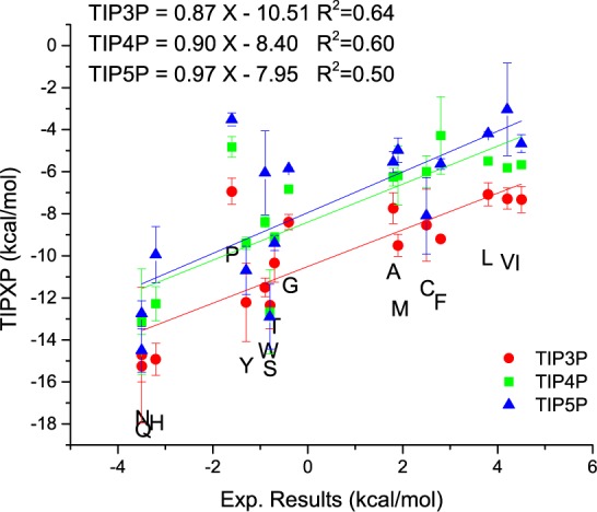
Free energy of solvation obtained with GIST compared to the hydrophobicity values from Kyte and Doolittle. Equations for the linear regression are given in the top left corner.
Figure 2 shows the free energy calculated with the presented method (y-axis) plotted against the values reported by Kyte and Doolittle (x-axis). The correlation between the two different scales is indicated by linear regression (R2-values > 0.50). Absolute values cannot be compared as the hydration of the backbone and the capping groups are also included in our scale. As the backbone and capping groups are always constraint to the same conformation the contribution to the thermodynamic quantities is nearly constant for all amino acids. This constant contribution to the free energy of hydration is responsible for the relative high value of the intercept. The results for glycine (G) and proline (P) differ from the experimental values. Most likely this arises because the distinction between side chain and backbone cannot be made as easily as for all other amino acids. When we exclude these two amino acids from the linear regression, we obtain R2-values between 0.74 and 0.92.
Again, our approach describes the transfer of a molecule from the vacuum to the aqueous phase. Although the distribution coefficients of molecules between the aqueous and the gas phase are an interesting molecular property, most of the frequently used scales describe the transfer of a molecule between an apolar environment, like octanol or a membrane, and a polar solvent like water.
Despite the fact that our scale neglects the interactions in the apolar solvent, the results are in a very good agreement with those of Kyte and Doolittle for nearly all amino acids. This finding is little surprising when looking at Kyte and Doolittle’s reference phase in more detail: This is an apolar, neutral, noninteracting solvent and only show van der Waals interactions. When an apolar molecule is solvated by this ideal apolar solvent, the surface area between apolar solvent molecules is reduced by the same amount as the surface area between the solute and the solvent molecules grows. As a first approximation we can assume that van der Waals interactions are similar between solute and solvent and between solvent molecules in an ideal apolar solvent. Therefore, the free energy of solvation in an ideal apolar solvent is negligible. Corrections of the obtained results with a term proportional to the solvent accessible surface area to account for the dispersion energy were found to be very small (<0.2 kcal/mol). As they could not significantly improve the results, we conclude that our assumption is valid: the free energy in an ideal apolar solvent is small compared to the free energy of solvation in a polar solvent.
From the free energy values it is not possible to identify which water model performs best. TIP3P has the highest correlation with experimental data, whereas the correct slope of nearly 1.0 is found for TIP5P.
Besides the hydrophobicity scale of Kyte and Doolittle a number of other scales exist. These scales are based on different experimental and bioinformatic measurements. Despite the variety of hydrophobicity scales, our proposed scale is the only one that focuses on the interactions between amino acids and their surrounding water molecules. For the sake of comparison Table 2 shows our hydrophobicity scale rank ordered for all 20 canonical amino acids and a selection of other published hydrophilicity scales.54−59 As all water models yield very similar results, resulting in the same rank order only the TIP3P based scale is depicted here.
Table 2. Rank Ordered Hydrophobicity Scale Proposed in This Work (GIST-TIP3P) in Comparison to Previously Published Hydrophobicity Scales.

The hydrophobicity scale of this work is in concordance with previously published scales. For all scales charged residues are found at the top end of the scale, as they are the most hydrophilic ones. The order of positive and negative charged residues are switched compared to all other scales. A possible reason is that the formation of the ion pair is neglected and solvation energies are reported. Also, the result for proline is different in our scale, but this can be explained with the unique property of proline: it has two chemical bonds connecting side chain and backbone. Therefore, it exerts a different influence of the backbone, which is most likely responsible for the deviation.
As mentioned above, one of the key advantages of our method is that the entropy can be obtained directly from a single simulation. As the hydrophobicity values from the previous paragraph cannot be split into an entropic and enthalpic part, our entropy and enthalpy results are compared to the experimental values (free energy, enthalpy, and entropy of hydration for the amino acid side chains) published by Privalov et al.60,61 (see Figure 3). Their reported values are based on the measurement of distribution coefficients of molecules between the aqueous phase and the gas phase.
Figure 3.

Free energy, enthalpy, and entropy values for all uncharged amino acids obtained with the GIST approach (y-axis) plotted against the experimentally obtained values (x-axis). The experimental values are free energies, enthalpy, and entropy of hydration reported by Privalov et al. Values are given in kcal/mol, and the equations for the linear regression are shown in the top left corner of every graph.
For nearly all amino acids free energies from theory and experiment agree well with each other (Pearson correlation coefficient between 0.96 and 0.82). Only for tryptophan differences between experiment and theory are found. For the enthalpic values the agreement is even better (Pearson correlation coefficient >0.94). Thus, we conclude that the different water models treat enthalpic effects similarly and accurately. Comparing experimental and theoretical entropy values reveal interesting differences. Especially for the aromatic amino acids (tryptophan W, tyrosine Y, phenylalanine F, and histidine H) calculated entropies are up to 5 kcal/mol higher than experimental values. The employed force field seems to overestimate the entropic penalty for solvation of aromatic rings. As tryptophan is the largest aromatic amino acid this overestimation is most likely the reason for the deviation between experimental and calculated ΔG. The difference could probably also be an artifact arising from too high point charges in the water models. To compensate for polarization occurring in real water the charges are set to higher values than they would occur in the isolated molecules or when water is surrounded by an apolar environment. With higher charges the entropy change gets underestimated because high charges will order water molecules in a more defined way. The mismatch between experimental and theoretical values is similar for all three tested water models. Polarizable water models could potentially improve this estimation.
The most common way to theoretically estimate thermodynamic properties of amino acid side chains is thermodynamic integration (TI). Similar to the described method, TI calculates the free energy gained by introducing/changing a group of the solute in solvent compared to the same transformation in the vacuum phase. From this point of view it is expected that TI results are very similar to the GIST-based results. Figure 4 shows a comparison of our results to the results obtained by Hajari with TI.15
Figure 4.

Free energy, enthalpy and entropy values for all uncharged amino acids obtained with the GIST approach (y-values) with respect to the values obtained by Hajari15 (x-values) with thermodynamic integration. The values of the linear regression for every water model are given in the top left corner.
The results from Hajari were obtained with the GROMOS 53A6 force field62 and the SPC63 water model. Despite the slightly different force field, the results are still in very good agreement with each other. The constant offset can be attributed to the contribution of the backbone atoms or differences due to conformational entropy of the solute. Especially for the TIP3P water model, results are nearly the same as with TI and the SPC water model, which is little surprising because the SPC and the TIP3P water models are very similar. Both water models are three-site water models with very similar properties. The differences in the results for the other two water models very likely arise from the different treatment of electrostatics. The good agreement suggests that both techniques TI and our GIST based hydrophobicity are capable of describing the change in free energy due to the solvation process and are equally correct (Similar results are also obtained for the enthalpy and entropy values.). We once more want to remind the reader that the presented scale includes an offset due to the inclusion of the backbone solvation. Therefore, only the relative values can be compared. Interestingly, we obtain slope values higher than 1.0 for the entropy. We would have expected values lower than 1.0 because GIST is neglecting higher order entropy terms. This may indicate that higher order entropy terms are small compared to the first order term and is in line with the results by Higgins et al., who stated that entropy is overestimated by IST calculations.38 While both TI and the presented hydrophobicity scale agree well with each other, our approach can obtain the entropy directly from the phase space water can occupy. Therefore, only one simulation is necessary to get the solvation entropy (for a rigid solute). For TI on the other hand, entropic changes are typically derived indirectly from the temperature dependence of the free energy (using multiple simulations at different temperatures) as done by Hajari et al.15 or via the difference of the free energy and the enthalpy. While Hajari et al. used 26 or more λ-values, 6 different temperatures, simulating every window for 5 ns, resulting in a total simulation time of ≥600 ns, we only needed 200 ns of simulation time (potentially even less without significant loss of accuracy).
Being able to measure entropic and enthalpic contributions allows a closer look at frequently discussed entropy-enthalpy compensation, the negative correlation between entropy and enthalpy of hydration. This negative correlation is also found in our theoretical calculations, as one may see in Figure 5: more negative values for the enthalpy, i.e., favorable enthalpic interactions are accompanied by high values for −TΔS, and thus an entropic penalty.
Figure 5.

Entropy-enthalpy compensation for uncharged amino acids obtained by the approach presented in this work: TIP3P (left), TIP4P (middle), TIP5P (right). Entropy is reported as −TΔS.
Although a negative correlation of the entropy and enthalpy is found overall, it is conspicuous that for all three water models polar amino acids tend to be found below the regression curve and apolar amino acids are found above. It may indicate that for polar amino acids the entropy-enthalpy compensation is rather small. The polar amino acids experience a smaller entropic penalty compared to apolar amino acids. Either this can be attributed to the simplistic treatment of electrostatics or entropy-enthalpy compensation is more pronounced at apolar surfaces. Alternatively, the shape of the apolar residues may lead to a different offset in the regression. The slope of the regressions for all water models ranges between 0.4 and 0.6 indicating that around half of the enthalpic interaction is compensated by entropy. It indicates that enthalpy and entropy are not perfectly correlated in simulations. Therefore, just looking at enthalpic values and neglecting the entropy can be misleading. Also, the entropy term (−TΔS) is in the same order of magnitude as the enthalpy, resulting in a significant contribution of the entropy to the free energy, which cannot be neglected.
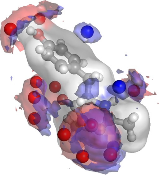
Our GIST based hydrophobicity scale provides not only entropy and enthalpy of solvation but also a spatial resolution of these quantities allowing for new insights into the hydrophobic character of amino acids side chains. It is possible to identify groups and/or functionalities that increase or decrease the hydration free energy. The implications of this are illustrated at the example of four amino acids depicted in Figure 6: it shows the spatial resolution of hydrophobicity obtained by analyses of the water environment around the amino acids.
Figure 6.
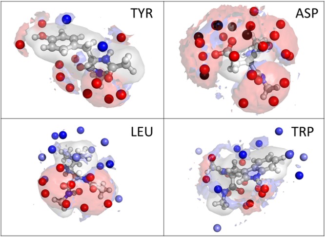
Representative examples of the spatial analysis of hydrophobicity around the four amino acids, tyrosine, aspartate, leucine, and tryptophan, with the presented method. Red areas show enthalpically favored water regions; blue areas show regions of low entropy (unfavorable). Red spheres represent maximum likelihood water positions with a negative contribution to the free energy (happy water molecules), whereas blue spheres show water positions with a positive (unfavorable) contribution (unhappy water molecule). Black spheres represent water positions with very high (>4 kcal/mol) negative contribution to the free energy (very happy water).
In Figure 6 red regions symbolize enthalpically favored positions for water molecules, whereas blue regions show entropic unfavorable positions. Almost all entropic unfavorable regions have their origin in a high enthalpic binding, known as the previous discussed entropy-enthalpy compensation. For tyrosine one position on top of the phenyl ring can be identified with a positive contribution to the free energy of hydration. This position shows entropically unfavorable behavior which is not compensated by additional enthalpic interactions. For aspartate very strong enthalpic interactions are found due to the charged group. Leucine and tryptophan show almost only positive contributions to the solvation free energy (visualized with blue spheres), which is expected for apolar amino acids. The interaction of the backbone is similar for all amino acids and show mostly negative contributions to the free energy. The presented examples show that this method produces reasonable results for all amino acids and can therefore also be used to analyze polypeptides and proteins. This provides a tool to predict the positions of water molecules and allows us to estimate the binding energy of these water molecules at protein surfaces or in pockets. Replacing loosely bound water molecules in proteins by a ligand can result in a significantly gain of binding free energy. Therefore, our methodology can be used in drug design studies to analyze the hydrophobicity of the binding site and to predict the change in free energy when bound waters are released into bulk and/or replaced by an inhibitor.
Conclusion
Enthalpic and entropic contributions to hydrophobicity of amino acid side chains were calculated by inhomogeneous solvation theory using a grid based approach. A hydrophobicity scale is presented, allowing for the determination of the thermodynamic properties for all 20 canonical amino acids. The presented scale based on interaction free energies can be especially helpful in cases, where the interaction energy between solute and solvent and/or the mobility of the solvent molecules is the variable of interest, e.g. for ice nucleation.64,65
For uncharged polar and apolar amino acids a good agreement with previously published experimental and theoretical hydrophobicity values was found. Therefore, the scale can also be used to determine the free energy for the transfer of a molecule from a polar to an apolar solvent. Our results also agree well with thermodynamic integration studies. However, the advantages of the GIST approach are (i) that it is possible to obtain with only one simulation the thermodynamic properties of interest resulting in shorter simulation time and (ii) that the entropy is calculated directly from the occupied phase space and not derived from multiple simulations. This allows us to analyze the spatial resolution of solvation thermodynamics as well as the individual contributions to it.
Comparison with experimental values showed a weakness of state-of-the-art water models and nonpolarizable force field calculations. The entropic effects are not described equally well as the enthalpic contributions. Especially for very apolar environments like aromatic side chains the charges of the water model are too high,66 and therefore the entropy penalty of solvation is overestimated. Nevertheless, the presented study showed that GIST is a valid approach to determine thermodynamic properties, especially relative differences in free energies and enthalpies, of amino acids. We conclude that our findings could be generalized, and our methodology may also be applied for the description of protein surfaces.
An additional advantage of the described method is the possibility to locate the differences in the thermodynamic properties of water molecules around the solute. This is probably only of minor importance when free energies for the transition of amino acids from water to octanol or to the gas phase are investigated but could be of interest when the method is used to investigate biomolecules70 as possible drug targets. It is very well-known that the hydration of binding sites plays a significant role in the binding processes of biomolecules.67,68 This study validates the GIST approach to describe thermodynamic changes in the water due to the presence of amino acids. Therefore, it is possible to identify areas of unfavorable bound waters. This information can be used improve the ligand binding by replacing so-called unhappy waters.
Acknowledgments
The authors thank the Austrian Science Fund (FWF) for funding of project P 23051.
Glossary
ABBREVIATIONS
- GIST
Grid Inhomogeneous Solvation Theory
- IST
Inhomogeneous Solvation Theory
- TI
Thermodynamic Integration
Supporting Information Available
The Supporting Information is available free of charge on the ACS Publications website at DOI: 10.1021/acs.jctc.6b00422.
Further decomposition of calculated thermodynamic properties: The total enthalpy is split in the interaction between the solute and the water and an enthalpy part describes the distortion of the water–water interactions. The entropy is split into an orientational and a translational part (PDF)
Author Contributions
The manuscript was written through contributions of all authors. All authors have given approval to the final version of the manuscript.
The authors declare no competing financial interest.
Supplementary Material
References
- Ben-Amotz D.; Underwood R. Unraveling Water’s Entropic Mysteries: A Unified View of Nonpolar, Polar, and Ionic Hydration. Acc. Chem. Res. 2008, 41 (8), 957–967. 10.1021/ar7001478. [DOI] [PubMed] [Google Scholar]
- Ball P. Water as an active constituent in cell biology. Chem. Rev. 2008, 108 (1), 74–108. 10.1021/cr068037a. [DOI] [PubMed] [Google Scholar]
- Kauzmann W. Some factors in the interpretation of protein denaturation. Adv. Protein Chem. 1959, 14, 1–63. 10.1016/S0065-3233(08)60608-7. [DOI] [PubMed] [Google Scholar]
- Lumry R.; Eyring H. Conformation Changes of Proteins. J. Phys. Chem. 1954, 58 (2), 110–120. 10.1021/j150512a005. [DOI] [Google Scholar]
- Beuming T.; Che Y.; Abel R.; Kim B.; Shanmugasundaram V.; Sherman W. Thermodynamic analysis of water molecules at the surface of proteins and applications to binding site prediction and characterization. Proteins: Struct., Funct., Genet. 2012, 80 (3), 871–883. 10.1002/prot.23244. [DOI] [PubMed] [Google Scholar]
- Ladbury J. E. Just add water! The effect of water on the specificity of protein-ligand binding sites and its potential application to drug design. Chem. Biol. 1996, 3 (12), 973–980. 10.1016/S1074-5521(96)90164-7. [DOI] [PubMed] [Google Scholar]
- Chandler D. Interfaces and the driving force of hydrophobic assembly. Nature 2005, 437 (7059), 640–647. 10.1038/nature04162. [DOI] [PubMed] [Google Scholar]
- Bakker H. J. Physical chemistry: Water’s response to the fear of water. Nature 2012, 491 (7425), 533–535. 10.1038/491533a. [DOI] [PubMed] [Google Scholar]
- Davis J. G.; Gierszal K. P.; Wang P.; Ben-Amotz D. Water structural transformation at molecular hydrophobic interfaces. Nature 2012, 491 (7425), 582–585. 10.1038/nature11570. [DOI] [PubMed] [Google Scholar]
- Kovacs J. M.; Mant C. T.; Hodges R. S. Determination of intrinsic hydrophilicity/hydrophobicity of amino acid side chains in peptides in the absence of nearest-neighbor or conformational effects. Biopolymers 2006, 84 (3), 283–297. 10.1002/bip.20417. [DOI] [PMC free article] [PubMed] [Google Scholar]
- Mant C. T.; Kovacs J. M.; Kim H.-M.; Pollock D. D.; Hodges R. S. Intrinsic amino acid side-chain hydrophilicity/hydrophobicity coefficients determined by reversed-phase high-performance liquid chromatography of model peptides: Comparison with other hydrophilicity/hydrophobicity scales. Biopolymers 2009, 92 (6), 573–595. 10.1002/bip.21316. [DOI] [PMC free article] [PubMed] [Google Scholar]
- Mazzé F. M.; Fuzo C. A.; Degrève L. A new amphipathy scale: I. Determination of the scale from molecular dynamics data. Biochim. Biophys. Acta, Proteins Proteomics 2005, 1747 (1), 35–46. 10.1016/j.bbapap.2004.09.019. [DOI] [PubMed] [Google Scholar]
- Sandberg L.; Edholm O. Calculated Solvation Free Energies of Amino Acids in a Dipolar Approximation. J. Phys. Chem. B 2001, 105 (1), 273–281. 10.1021/jp002110y. [DOI] [Google Scholar]
- MacCallum J. L.; Tieleman D. P. Hydrophobicity scales: a thermodynamic looking glass into lipid–protein interactions. Trends Biochem. Sci. 2011, 36 (12), 653–662. 10.1016/j.tibs.2011.08.003. [DOI] [PubMed] [Google Scholar]
- Hajari T.; van der Vegt N. F. A. Solvation thermodynamics of amino acid side chains on a short peptide backbone. J. Chem. Phys. 2015, 142 (14), 144502. 10.1063/1.4917076. [DOI] [PubMed] [Google Scholar]
- Peter C.; Oostenbrink C.; van Dorp A.; van Gunsteren W. F. Estimating entropies from molecular dynamics simulations. J. Chem. Phys. 2004, 120 (6), 2652–2661. 10.1063/1.1636153. [DOI] [PubMed] [Google Scholar]
- Laage D.; Stirnemann G.; Hynes J. T. Why Water Reorientation Slows without Iceberg Formation around Hydrophobic Solutes. J. Phys. Chem. B 2009, 113 (8), 2428–2435. 10.1021/jp809521t. [DOI] [PubMed] [Google Scholar]
- Frank H. S.; Evans M. W. Free Volume and Entropy in Condensed Systems III. Entropy in Binary Liquid Mixtures; Partial Molal Entropy in Dilute Solutions; Structure and Thermodynamics in Aqueous Electrolytes. J. Chem. Phys. 1945, 13 (11), 507–532. 10.1063/1.1723985. [DOI] [Google Scholar]
- Ishihara Y.; Okouchi S.; Uedaira H. Dynamics of hydration of alcohols and diols in aqueous solutions. J. Chem. Soc., Faraday Trans. 1997, 93 (18), 3337–3342. 10.1039/a701969f. [DOI] [Google Scholar]
- Bagchi B. Water Dynamics in the Hydration Layer around Proteins and Micelles. Chem. Rev. 2005, 105 (9), 3197–3219. 10.1021/cr020661+. [DOI] [PubMed] [Google Scholar]
- Makarov V. A.; Feig M.; Andrews B. K.; Pettitt B. M. Diffusion of Solvent around Biomolecular Solutes: A Molecular Dynamics Simulation Study. Biophys. J. 1998, 75 (1), 150–158. 10.1016/S0006-3495(98)77502-2. [DOI] [PMC free article] [PubMed] [Google Scholar]
- Brooks C. L.; Karplus M. Solvent effects on protein motion and protein effects on solvent motion. J. Mol. Biol. 1989, 208 (1), 159–181. 10.1016/0022-2836(89)90093-4. [DOI] [PubMed] [Google Scholar]
- Bizzarri A. R.; Cannistraro S. Molecular Dynamics of Water at the Protein–Solvent Interface. J. Phys. Chem. B 2002, 106 (26), 6617–6633. 10.1021/jp020100m. [DOI] [Google Scholar]
- Yoshida K.; Ibuki K.; Ueno M. Pressure and temperature effects on 2H spin-lattice relaxation times and 1H chemical shifts in tert-butyl alcohol- and urea-D2O solutions. J. Chem. Phys. 1998, 108 (4), 1360–1367. 10.1063/1.475509. [DOI] [Google Scholar]
- Lumry R.; Rajender S. Enthalpy-entropy compensation phenomena in water solutions of proteins and small molecules: a ubiquitous property of water. Biopolymers 1970, 9 (10), 1125–1227. 10.1002/bip.1970.360091002. [DOI] [PubMed] [Google Scholar]
- Rezus Y. L. A.; Bakker H. J. Observation of immobilized water molecules around hydrophobic groups. Phys. Rev. Lett. 2007, 99 (14), 148301. 10.1103/PhysRevLett.99.148301. [DOI] [PubMed] [Google Scholar]
- Guillot B.; Guissani Y. A computer simulation study of the temperature dependence of the hydrophobic hydration. J. Chem. Phys. 1993, 99 (10), 8075–8094. 10.1063/1.465634. [DOI] [Google Scholar]
- Lee B. Enthalpy-entropy compensation in the thermodynamics of hydrophobicity. Biophys. Chem. 1994, 51 (2–3), 271–278. 10.1016/0301-4622(94)00048-4. [DOI] [PubMed] [Google Scholar]
- Galamba N. Water’s Structure around Hydrophobic Solutes and the Iceberg Model. J. Phys. Chem. B 2013, 117 (7), 2153–2159. 10.1021/jp310649n. [DOI] [PubMed] [Google Scholar]
- Titantah J. T.; Karttunen M. Long-Time Correlations and Hydrophobe-Modified Hydrogen-Bonding Dynamics in Hydrophobic Hydration. J. Am. Chem. Soc. 2012, 134 (22), 9362–9368. 10.1021/ja301908a. [DOI] [PubMed] [Google Scholar]
- Rossato L.; Rossetto F.; Silvestrelli P. L. Aqueous Solvation of Methane from First Principles. J. Phys. Chem. B 2012, 116 (15), 4552–4560. 10.1021/jp300774z. [DOI] [PubMed] [Google Scholar]
- Bakulin A. A.; Pshenichnikov M. S.; Bakker H. J.; Petersen C. Hydrophobic Molecules Slow Down the Hydrogen-Bond Dynamics of Water. J. Phys. Chem. A 2011, 115 (10), 1821–1829. 10.1021/jp107881j. [DOI] [PubMed] [Google Scholar]
- Qvist J.; Halle B. Thermal Signature of Hydrophobic Hydration Dynamics. J. Am. Chem. Soc. 2008, 130 (31), 10345–10353. 10.1021/ja802668w. [DOI] [PubMed] [Google Scholar]
- Wachter W.; Buchner R.; Hefter G. Hydration of Tetraphenylphosphonium and Tetraphenylborate Ions by Dielectric Relaxation Spectroscopy. J. Phys. Chem. B 2006, 110 (10), 5147–5154. 10.1021/jp057189r. [DOI] [PubMed] [Google Scholar]
- Huber R. G.; Fuchs J. E.; von Grafenstein S.; Laner M.; Wallnoefer H. G.; Abdelkader N.; Kroemer R. T.; Liedl K. R. Entropy from State Probabilities: Hydration Entropy of Cations. J. Phys. Chem. B 2013, 117 (21), 6466–6472. 10.1021/jp311418q. [DOI] [PMC free article] [PubMed] [Google Scholar]
- Åqvist J.; Hansson T. On the Validity of Electrostatic Linear Response in Polar Solvents. J. Phys. Chem. 1996, 100 (22), 9512–9521. 10.1021/jp953640a. [DOI] [Google Scholar]
- Gallicchio E.; Kubo M. M.; Levy R. M. Enthalpy-Entropy and Cavity Decomposition of Alkane Hydration Free Energies: Numerical Results and Implications for Theories of Hydrophobic Solvation. J. Phys. Chem. B 2000, 104 (26), 6271–6285. 10.1021/jp0006274. [DOI] [Google Scholar]
- Paschek D. Temperature dependence of the hydrophobic hydration and interaction of simple solutes: An examination of five popular water models. J. Chem. Phys. 2004, 120 (14), 6674–6690. 10.1063/1.1652015. [DOI] [PubMed] [Google Scholar]
- Huggins D. J.; Payne M. C. Assessing the Accuracy of Inhomogeneous Fluid Solvation Theory in Predicting Hydration Free Energies of Simple Solutes. J. Phys. Chem. B 2013, 117 (27), 8232–8244. 10.1021/jp4042233. [DOI] [PMC free article] [PubMed] [Google Scholar]
- Hess B.; van der Vegt N. F. A. Hydration Thermodynamic Properties of Amino Acid Analogues: A Systematic Comparison of Biomolecular Force Fields and Water Models. J. Phys. Chem. B 2006, 110 (35), 17616–17626. 10.1021/jp0641029. [DOI] [PubMed] [Google Scholar]
- Matysiak S.; Debenedetti P. G.; Rossky P. J. Dissecting the Energetics of Hydrophobic Hydration of Polypeptides. J. Phys. Chem. B 2011, 115 (49), 14859–14865. 10.1021/jp2079633. [DOI] [PubMed] [Google Scholar]
- Khoury G. A.; Bhatia N.; Floudas C. A. Hydration free energies calculated using the AMBER ff03 charge model for natural and unnatural amino acids and multiple water models. Comput. Chem. Eng. 2014, 71, 745–752. 10.1016/j.compchemeng.2014.07.017. [DOI] [Google Scholar]
- König G.; Boresch S. Hydration Free Energies of Amino Acids: Why Side Chain Analog Data Are Not Enough. J. Phys. Chem. B 2009, 113 (26), 8967–8974. 10.1021/jp902638y. [DOI] [PubMed] [Google Scholar]
- Hajari T.; van der Vegt N. F. A. Peptide Backbone Effect on Hydration Free Energies of Amino Acid Side Chains. J. Phys. Chem. B 2014, 118 (46), 13162–13168. 10.1021/jp5094146. [DOI] [PubMed] [Google Scholar]
- Nguyen C. N.; Cruz A.; Gilson M. K.; Kurtzman T. Thermodynamics of Water in an Enzyme Active Site: Grid-Based Hydration Analysis of Coagulation Factor Xa. J. Chem. Theory Comput. 2014, 10 (7), 2769–2780. 10.1021/ct401110x. [DOI] [PMC free article] [PubMed] [Google Scholar]
- Nguyen C. N.; Young T. K.; Gilson M. K. Grid inhomogeneous solvation theory: hydration structure and thermodynamics of the miniature receptor cucurbit [7] uril. J. Chem. Phys. 2012, 137 (4), 044101. 10.1063/1.4733951. [DOI] [PMC free article] [PubMed] [Google Scholar]
- Case D. A.; Berryman J. T.; Betz R. M.; Cerutti D. S.; Cheatham T. E. III; Darden T. A.; Duke R. E.; Giese T. J.; Gohlke H.; Goetz A. W.; Homeyer N.; Izadi S.; Janowski P.; Kaus J.; Kovalenko A.; Lee T. S.; LeGrand S.; Li P.; Luchko T.; Luo R.; Madej B.; Merz K. M.; Monard G.; Needham P.; Nguyen H.; Nguyen H. T.; Omelyan I.; Onufriev A.; Roe D. R.; Roitberg A.; Salomon-Ferrer R.; Simmerling C. L.; Smith W.; Swails J.; Walker R. C.; Wang J.; Wolf R. M.; Wu X.; York D. M.; Kollman P. A.. AMBER 2015; University of California: San Francisco, 2015.
- Nguyen C. N.; Kurtzman T.; Gilson M. K. Spatial Decomposition of Translational Water–Water Correlation Entropy in Binding Pockets. J. Chem. Theory Comput. 2016, 12 (1), 414–429. 10.1021/acs.jctc.5b00939. [DOI] [PMC free article] [PubMed] [Google Scholar]
- Vega C.; Abascal J. L. F. Simulating water with rigid non-polarizable models: a general perspective. Phys. Chem. Chem. Phys. 2011, 13 (44), 19663–19688. 10.1039/c1cp22168j. [DOI] [PubMed] [Google Scholar]
- Jorgensen W. L.; Chandrasekhar J.; Madura J. D.; Impey R. W.; Klein M. L. Comparison of simple potential functions for simulating liquid water. J. Chem. Phys. 1983, 79 (2), 926–935. 10.1063/1.445869. [DOI] [Google Scholar]
- Mahoney M. W.; Jorgensen W. L. A five-site model for liquid water and the reproduction of the density anomaly by rigid, nonpolarizable potential functions. J. Chem. Phys. 2000, 112 (20), 8910–8922. 10.1063/1.481505. [DOI] [Google Scholar]
- Wallnoefer H. G.; Handschuh S.; Liedl K. R.; Fox T. Stabilizing of a Globular Protein by a Highly Complex Water Network: A Molecular Dynamics Simulation Study on Factor Xa. J. Phys. Chem. B 2010, 114 (21), 7405–7412. 10.1021/jp101654g. [DOI] [PubMed] [Google Scholar]
- Kelly C. P.; Cramer C. J.; Truhlar D. G. Aqueous Solvation Free Energies of Ions and Ion–Water Clusters Based on an Accurate Value for the Absolute Aqueous Solvation Free Energy of the Proton. J. Phys. Chem. B 2006, 110 (32), 16066–16081. 10.1021/jp063552y. [DOI] [PubMed] [Google Scholar]
- Stover M. L.; Jackson V. E.; Matus M. H.; Adams M. A.; Cassady C. J.; Dixon D. A. Fundamental Thermochemical Properties of Amino Acids: Gas-Phase and Aqueous Acidities and Gas-Phase Heats of Formation. J. Phys. Chem. B 2012, 116 (9), 2905–2916. 10.1021/jp207271p. [DOI] [PubMed] [Google Scholar]
- Kyte J.; Doolittle R. F. A simple method for displaying the hydropathic character of a protein. J. Mol. Biol. 1982, 157 (1), 105–132. 10.1016/0022-2836(82)90515-0. [DOI] [PubMed] [Google Scholar]
- Engelman D. M.; Steitz T. A.; Goldman A. Identifying nonpolar transbilayer helices in amino acid sequences of membrane proteins. Annu. Rev. Biophys. Biophys. Chem. 1986, 15, 321–353. 10.1146/annurev.bb.15.060186.001541. [DOI] [PubMed] [Google Scholar]
- Eisenberg D.; Schwarz E.; Komaromy M.; Wall R. Analysis of membrane and surface protein sequences with the hydrophobic moment plot. J. Mol. Biol. 1984, 179 (1), 125–142. 10.1016/0022-2836(84)90309-7. [DOI] [PubMed] [Google Scholar]
- Janin J. Surface and inside volumes in globular proteins. Nature 1979, 277 (5696), 491–492. 10.1038/277491a0. [DOI] [PubMed] [Google Scholar]
- Cornette J. L.; Cease K. B.; Margalit H.; Spouge J. L.; Berzofsky J. A.; DeLisi C. Hydrophobicity scales and computational techniques for detecting amphipathic structures in proteins. J. Mol. Biol. 1987, 195 (3), 659–685. 10.1016/0022-2836(87)90189-6. [DOI] [PubMed] [Google Scholar]
- Hopp T. P.; Woods K. R. A computer program for predicting protein antigenic determinants. Mol. Immunol. 1983, 20 (4), 483–489. 10.1016/0161-5890(83)90029-9. [DOI] [PubMed] [Google Scholar]
- Makhatadze G. I.; Privalov P. L. Contribution of Hydration to Protein Folding Thermodynamics: I. The Enthalpy of Hydration. J. Mol. Biol. 1993, 232 (2), 639–659. 10.1006/jmbi.1993.1416. [DOI] [PubMed] [Google Scholar]
- Privalov P. L.; Makhatadze G. I. Contribution of Hydration to Protein Folding Thermodynamics: II. The Entropy and Gibbs Energy of Hydration. J. Mol. Biol. 1993, 232 (2), 660–679. 10.1006/jmbi.1993.1417. [DOI] [PubMed] [Google Scholar]
- Oostenbrink C.; Villa A.; Mark A. E.; van Gunsteren W. F. A biomolecular force field based on the free enthalpy of hydration and solvation: the GROMOS force-field parameter sets 53A5 and 53A6. J. Comput. Chem. 2004, 25 (13), 1656–1676. 10.1002/jcc.20090. [DOI] [PubMed] [Google Scholar]
- Berendsen H. J. C.; Postma J. P. M.; Gunsteren W. F.; Hermans J.. Interaction Models for Water in Relation to Protein Hydration. In Intermol. Forces: Proceedings of the Fourteenth Jerusalem Symposium on Quantum Chemistry and Biochemistry Held in Jerusalem, Israel, April 13–16, 1981, Pullman B., Ed.; Springer: Netherlands: Dordrecht, 1981; pp 331–342. [Google Scholar]
- Pummer B. G.; Budke C.; Augustin-Bauditz S.; Niedermeier D.; Felgitsch L.; Kampf C. J.; Huber R. G.; Liedl K. R.; Loerting T.; Moschen T.; Schauperl M.; Tollinger M.; Morris C. E.; Wex H.; Grothe H.; Pöschl U.; Koop T.; Fröhlich-Nowoisky J. Ice nucleation by water-soluble macromolecules. Atmos. Chem. Phys. 2015, 15 (8), 4077–4091. 10.5194/acp-15-4077-2015. [DOI] [Google Scholar]
- Cox S. J.; Kathmann S. M.; Slater B.; Michaelides A. Molecular simulations of heterogeneous ice nucleation. I. Controlling ice nucleation through surface hydrophilicity. J. Chem. Phys. 2015, 142 (18), 184704. 10.1063/1.4919714. [DOI] [PubMed] [Google Scholar]
- Halgren T. A.; Damm W. Polarizable force fields. Curr. Opin. Struct. Biol. 2001, 11 (2), 236–242. 10.1016/S0959-440X(00)00196-2. [DOI] [PubMed] [Google Scholar]
- Raman E. P.; MacKerell A. D. Spatial Analysis and Quantification of the Thermodynamic Driving Forces in Protein-Ligand Binding: Binding Site Variability. J. Am. Chem. Soc. 2015, 137 (7), 2608–2621. 10.1021/ja512054f. [DOI] [PMC free article] [PubMed] [Google Scholar]
- Patel A. J.; Varilly P.; Jamadagni S. N.; Hagan M. F.; Chandler D.; Garde S. Sitting at the Edge: How Biomolecules use Hydrophobicity to Tune their Interactions and Function. J. Phys. Chem. B 2012, 116 (8), 2498–2503. 10.1021/jp2107523. [DOI] [PMC free article] [PubMed] [Google Scholar]
- Biedermann F.; Uzunova V. D.; Scherman O. A.; Nau W. M.; De Simone A. Release of high-energy water as an essential driving force for the high-affinity binding of cucurbit[n]urils. J. Am. Chem. Soc. 2012, 134 (37), 15318–15323. 10.1021/ja303309e. [DOI] [PubMed] [Google Scholar]
Associated Data
This section collects any data citations, data availability statements, or supplementary materials included in this article.