Do abundance distributions and species aggregation correctly predict macroecological biodiversity patterns in tropical forests?

Abstract

Aim

It has been recently suggested that different ‘unified theories of biodiversity and biogeography’ can be characterized by three common ‘minimal sufficient rules’: (1) species abundance distributions follow a hollow curve, (2) species show intraspecific aggregation, and (3) species are independently placed with respect to other species. Here, we translate these qualitative rules into a quantitative framework and assess if these minimal rules are indeed sufficient to predict multiple macroecological biodiversity patterns simultaneously.

Location

Tropical forest plots in Barro Colorado Island (BCI), Panama, and in Sinharaja, Sri Lanka.

Methods

We assess the predictive power of the three rules using dynamic and spatial simulation models in combination with census data from the two forest plots. We use two different versions of the model: (1) a neutral model and (2) an extended model that allowed for species differences in dispersal distances. In a first step we derive model parameterizations that correctly represent the three minimal rules (i.e. the model quantitatively matches the observed species abundance distribution and the distribution of intraspecific aggregation). In a second step we applied the parameterized models to predict four additional spatial biodiversity patterns.

Results

Species‐specific dispersal was needed to quantitatively fulfil the three minimal rules. The model with species‐specific dispersal correctly predicted the species–area relationship, but failed to predict the distance decay, the relationship between species abundances and aggregations, and the distribution of a spatial co‐occurrence index of all abundant species pairs. These results were consistent over the two forest plots.

Main conclusions

The three ‘minimal sufficient’ rules only provide an incomplete approximation of the stochastic spatial geometry of biodiversity in tropical forests. The assumption of independent interspecific placements is most likely violated in many forests due to shared or distinct habitat preferences. Furthermore, our results highlight missing knowledge about the relationship between species abundances and their aggregation.

Introduction

Explaining the commonness and rarity of species as well as their distributions in space are central questions in biodiversity science and biogeography (Brown et al., 1995; Rosenzweig, 1995). One important goal of modern ecology is therefore the development of a unified theory that predicts species abundances and distributions for a wide range of ecosystems and taxa (Hubbell, 2001; Chase, 2005; Harte et al., 2008).

Recently, McGill (2010) reviewed six ecological theories that were intended to predict from a few underlying principles several patterns in macroecology and biogeography, such as the species abundance distribution (SAD; McGill et al., 2007) and spatial biodiversity patterns, in particular the species–area relationship (SAR; Rosenzweig, 1995) and the distance decay of community similarity (F(r); Condit et al., 2002; Morlon et al., 2008). The theories reviewed by McGill (2010) include dynamic approaches, for example spatially implicit (Hubbell, 2001) and spatially explicit neutral models (Chave & Leigh, 2002) that were built from the assumptions of species per capita equivalence, dispersal limitation and zero‐sum dynamics (Hubbell, 2001). The theories also include static approaches such as Poisson‐cluster models (e.g. Plotkin et al., 2000; Morlon et al., 2008) where fitted point‐process models mimic the observed clustered distribution pattern of each species individually without reference to the underlying demographic and spatial processes. Independent superposition of species patterns then produces the predicted communities (Wiegand & Moloney, 2014). It has been shown that Poisson‐cluster models can approximate the SAR and distance decay in forest communities (e.g. Morlon et al., 2008; Wang et al., 2011).

Despite superficial differences in the mathematical formulation and target spatial scales of the reviewed theories, McGill (2010) suggested that all of them share three common assertions or ‘minimal sufficient rules’ (McGill, 2010, p. 633).

1. Individuals of the same species are aggregated in space.

2. Abundance between species varies drastically and the abundance distribution shows a hollow curve, when the number of species is counted in abundance classes on a linear scale, i.e. there are many rare and just a few common species.

3. Individuals of different species can be treated as independent and placed without regard to other species.

According to McGill (2010) these three rules should allow, in combination with spatial and temporal stochasticity, the prediction of at least two major macroecological biodiversity patterns, namely the SAR and the distance decay of community similarity. However, the three rules are formulated in a qualitative manner and it remains an open question of how to translate them into quantitative rules and how to use them to derive predictions of spatial biodiversity patterns.

The simultaneous prediction of multiple observed patterns has been suggested as an important test of any model or theory (Wiegand et al., 2003; Grimm et al., 2005; McGill et al., 2007). Ultimately, only a theory that provides multiple realistic predictions of biodiversity patterns qualifies as a ‘unifying theory of biodiversity’. All six theories reviewed by McGill (2010) are indeed able to predict biodiversity patterns correctly (see Table 2 in McGill, 2010). However, previous tests of these theories often focused on single patterns and rarely assessed whether multiple patterns can be correctly predicted with one model and one set of parameters (but see Jabot & Chave, 2009; Horvat et al., 2010; May et al., 2015).

In this study we demonstrate how the three qualitative rules can be translated into a quantitative framework, and we assess the predictive power of the three rules for several macroecological biodiversity patterns, including: (1) the SAR, (2) the distance decay, (3) the spatial co‐occurrence or segregation of species pairs (Wiegand et al., 2007, 2012), and (4) the relationship between intraspecific aggregation and species abundances (He et al., 1997; Condit et al., 2000; Plotkin et al., 2000). For this purpose we used a dynamic and spatially explicit simulation model in combination with census data from two large tropical forest plots in Panama and Sri Lanka. To allow for a quantitative comparison of observed and simulated patterns we used the spatial simulation model CONFETTI (May et al., 2015) in which each tree is characterized by an explicit position in continuous space rather than on a discrete lattice (e.g. Chave et al., 2002; Rosindell & Cornell, 2009; May et al., 2012). CONFETTI includes the key processes of tree mortality, local recruitment and immigration from the metacommunity (May et al., 2015). We used two versions of the model, which both fulfil rule 3 of interspecific independence (i.e. there are no shared or distinct habitat preferences, Janzen–Connell effects or competitive hierarchies): (1) a neutral model version without species‐specific differences and (2) an extended version of the model where species can differ in their dispersal distances. The latter may be necessary to correctly predict the observed distribution of species aggregation (rule 1) (Plotkin et al., 2000).

In the first step of our analysis we used inverse modelling (Hartig et al., 2011) and the spatial data from the two tropical forest plots to search parameterizations of the two model versions that quantitatively fulfil the three rules of McGill (2010). In a second step we tested if the parameterized simulation models are able to quantitatively predict the four additional patterns mentioned above.

With this approach we aimed to answer the following specific questions.

1. Is the neutral model version able to simultaneously predict the distributions of species abundances and of intraspecific aggregation, or are species‐specific dispersal kernels needed for this?

2. Is a model that quantitatively fulfils the three minimal sufficient rules able to correctly predict several additional macroecological biodiversity patterns?

3. Does the ability of the models to predict multiple patterns differ between the two contrasting tropical forests?

Our study suggests that the three rules proposed by McGill (2010) provide only an incomplete approximation of the stochastic spatial geometry of biodiversity and that additional processes are required to predict the key macroecological biodiversity patterns simultaneously. Our results points to specific extensions of existing biodiversity theories to improve our general understanding of the dynamics of species‐rich communities.

Methods

Study sites

We used census data from two tropical forest dynamics plots, Barro Colorado Island (BCI) in Panama (Hubbell et al., 1999, 2005) and Sinharaja in Sri Lanka (Gunatilleke et al., 2004a, 2004b). The 50‐ha forest plot at BCI (9°9′ N, 79°51′ W) represents seasonally moist tropical forest with a pronounced dry season and a mean annual rainfall of 2600 mm. The plot comprises old growth lowland moist forest and contains up to 305 tree and shrub species. Elevation in the plot ranges from 120 to 155 m a.s.l. The plot was established in 1982 and all trees with a diameter at breast height (d.b.h.) ≥ 1 cm have been mapped, tagged and measured every 5 years since 1985 (Condit, 1998; Hubbell et al., 2005).

The 25‐ha plot at the Sinharaja UNESCO World Heritage Site in Sri Lanka (6°24′ N, 80°24′ E) contains tropical wet forest without a distinct dry season and has a mean annual rainfall of 5016 mm. Elevation in the plot ranges from 424 to 575 m a.s.l. and includes a valley lying between two slopes. The forest represents a mixed dipterocarp forest (Ashton, 1964; Whitmore, 1984) and includes 220 woody species. All trees with d.b.h. ≥ 1 cm have been mapped, tagged and measured every 5 years since 1996 (Gunatilleke et al., 2006).

Dynamic and spatially explicit community model

The stochastic simulation model used for this study is an adapted version of the model CONFETTI, which dynamically simulates survival, mortality, recruitment and immigration of all adult trees in a tropical forest plot (May et al., 2015). The model structure was inspired by previous plant community models (Hubbell, 2001; Chave & Leigh, 2002) and combines a spatially implicit metacommunity with a spatially explicit local community (Fig. 1). In contrast to previous spatial community models (e.g. Chave et al., 2002; Rosindell & Cornell, 2009; May et al., 2012), individual trees in CONFETTI are described in continuous space rather than on a discrete two‐dimensional lattice. This is necessary to take full advantage of the spatial census data and to allow for a direct comparison of field data and model output using summary statistics derived by spatial point‐pattern analysis (Wiegand & Moloney, 2014) to characterize the stochastic spatial geometry of biodiversity. We used two different versions of the model: a simplified version of the neutral model of May et al. (2015) and an extended version that allows additionally for interspecific differences in dispersal distances. In the following we present a summary of the simulation model, while a detailed description is provided in the Supporting Information (Appendix S1).

Figure 1.

General structure of the of the CONFETTI model. The non‐spatial metacommunity is characterized by a constant rank–abundance curve, which is simulated based on a fundamental biodiversity number (θ) and the number of individual trees (J_M) (Hubbell, 2001). In the spatially explicit local community each point represents a tree, which is described by its position in space (x–y coordinates) and its species identity (shade of grey). Here only a subplot of 200 m × 100 m is shown. The local community is linked to the metacommunity by immigration of tree recruits. In the local community we assume zero‐sum dynamics, i.e. the number of individual trees remains constant over time. See the main text and Appendix S1 for a more detailed model description.

In the beginning of each simulation the static and non‐spatial metacommunity was generated (Hubbell, 2001, p. 289; Etienne & Alonso, 2005). The abundance distributions and the diversity of the metacommunity were determined by the fundamental biodiversity number θ (Hubbell, 2001). The spatially explicit local community represents a forest plot of the size of 50 ha (BCI) or 25 ha (Sinharaja). We assume zero‐sum dynamics, i.e. the number of trees was constant over time and was fixed to the average number of trees with d.b.h. ≥ 10 cm in BCI (21,000) or Sinharaja (17,500). Tree mortality was simulated as a random event and all tree species shared the same mortality rate, equal to the observed annual mortality of trees with d.b.h. ≥ 10 cm (c. 2%). This corresponds to a mean tree age of c. 50 years. As soon as a tree died, a new individual tree, called ‘recruit’, was generated either as immigrant from the metacommunity (with probability m) or as offspring of another tree in the local community (with probability 1 – m). The parameter m is called the immigration rate (Hubbell, 2001).

Local recruitment was modelled using a log‐normal kernel for the dispersal distance (Greene et al., 2004; May et al., 2012). Note that ‘recruitment’ refers here to the establishment of a new adult tree. Since neutral models typically consider only reproductive adults (Hubbell, 2001), we model only the dynamics of reproductive trees, which are here represented by trees larger than 10 cm d.b.h. We used the common 10‐cm d.b.h. threshold (e.g. Hubbell, 2001, Rosindell & Cornell, 2009) because no data on reproductive thresholds were available for the Sinharaja forest plot. The distribution of the mean dispersal distances among species was also modelled by a log‐normal distribution (Muller‐Landau et al., 2008) with mean d _m and standard deviation d _sd as model parameters.

The sequence of birth–death events was iterated for 100 generations (c. 5000 years). At the end of each simulation run we recorded one virtual forest census that was used to calculate the macroecological biodiversity patterns described below.

Model parameterization

In the first step of our analysis, we required that the models should quantitatively fulfil the three unifying rules of McGill (2010). Since rule 3 (interspecific independence) is fulfilled by definition, we used inverse modelling techniques (Wiegand et al., 2003; Beaumont, 2010; Hartig et al., 2011) to find model parameterizations that predict quantitatively realistic species‐specific aggregation (rule 1) and SADs (rule 2).

As summary statistics to quantify species aggregation we used species‐specific aggregation indices M_i(r) based on Ripley's K, where

$$M_i\left(r\right)={\log }_{10}\left[K_i\left(r\right)/\pi r^2)\right].$$ (1)

The M_i(r) were evaluated for all species with at least 50 tree individuals (Condit et al., 2000). The K‐function K_i(r) of species i was estimated as the mean number of conspecific trees within radius r, divided by the overall density λ_i of the focal species i in the plot (Wiegand & Moloney, 2014). The expected value of K_i(r) for a completely random pattern equals K_i(r) = πr ². We used log₁₀‐transformed values and scaling with the expected value for easy interpretation of the M_i(r) values (Wiegand et al., 2012). M_i(r) > 0 indicates species aggregation, while M_i(r) < 0 indicates regular patterns. As M_i(r) is a scale‐dependent measure and we aimed for a correct representation of intraspecific aggregation at several scales, we calculated M_i(r) for r = 10 m and r = 50 m.

The final set of summary statistics used for parameter estimation included: (1) the total species richness of the local community, (2) the SAD with logarithmic abundance classes (Hubbell, 2001), and the means (3) and standard deviations (4) of the distribution of the intraspecific aggregation indices M_i(r), with r = 10 m and r = 50 m. For the field data we evaluated these six summary statistics for all available forest censuses (1985–2010 for BCI and 1996–2001 for Sinharaja) using all living trees with d.b.h. ≥ 10 cm. Finally, we averaged the summary statistics over the different censuses for each plot. In the model simulations we derived the summary statistics from a virtual forest census of at the end of the simulation run of 100 tree generations.

We used global stochastic optimization to find model parameterizations that produced the best match between observed and simulated summary statistics (Zhang & Sanderson, 2009; Lehmann & Huth, 2015). Model fitting was done separately for the two versions of the model (i.e. the neutral model and the extended model with species‐specific dispersal) and the two forest plots. For the neutral model the standard deviation of dispersal distances among species (d _sd) was set to zero, and the parameters that were varied during the optimization included the fundamental biodiversity number (θ), the immigration rate (m) and the mean dispersal distance of all species (d _m). In the extended model version we additionally estimated d _sd during the optimization. More details on the parameter optimization are provided in Appendix S1.

Model validation and predictions

To answer our first question (i.e. to find out if the parameterized models were able to quantitatively predict the observed species aggregation and SAD), we conducted model simulations with the 1000 best parameter sets obtained from the optimization and calculated the distribution of the six summary statistics that were used for parameter estimation.

To answer our second question (i.e. whether a model that quantitatively fulfils the three rules is able to correctly predict several additional spatial biodiversity patterns) we investigated if the parameterized models were able to provide independent predictions of patterns that were not used for parameter estimation. For this purpose we estimated the four additional patterns of the stochastic spatial geometry of biodiversity explained below from the same 1000 model runs and compared them with the corresponding values derived from the forest census data.

The first pattern is the SAR, which was calculated as the average number of species in non‐overlapping quadrats (or rectangles) ranging from 1 m² to the size of the entire plot. The second pattern is the distance decay of community similarity based on the proportion of conspecific neighbours F(r). F(r) is defined as the probability that two randomly chosen trees at distance r belong to the same species (Chave & Leigh, 2002). It can be expressed in terms of the pair correlation functions g_i(r) and g(r) of species i and of all individuals, respectively, as

$$F\left(r\right)={\displaystyle \sum _{i=1}^S{f}_i^2\frac{g_i\left(r\right)}{g\left(r\right)}},$$ (2)

where S is the total number of species, f_i = n_i/n is the relative abundance of species i and the pair correlation function g(r) is the non‐cumulative version of the K‐function, i.e.

$$K_i\left(r\right)={\displaystyle {\int }_{t=0}^r{g}_i\left(r\right)2\pi t\mathrm{d}t}.$$ (3)

The larger the value of g_i(r), the larger the aggregation of species i. Thus, F(r) is strongly influenced by the correlation between species abundances f_i and intraspecific aggregation represented by g_i(r) (Wiegand & Moloney, 2014). However, because F(r) is conditional on the pattern of all individuals (i.e. division by g(r)), it is also influenced by species co‐occurrence patterns (Wang et al., 2015). We evaluated F(r) at distances r ranging from 1 to 50 m.

As third pattern, we used the relationship between the abundance n_i of species i and its intraspecific aggregation. For this purpose, we calculated the Spearman rank‐correlation between n_i and the aggregation M_i(r) of all species i (equation (1)) with at least 50 individuals.

To assess if our results depend on the specific aggregation index M_i(r) used (which is based on the neighbourhood tree density within distance r), we also used the species‐specific nearest‐neighbour clumping index CI_i = r_i ^a/r_i ^c used by He et al. (1997), where r_i ^a is the observed (or simulated) mean distance to the nearest conspecific neighbour and r_i ^c is the corresponding value of a spatially random pattern. CI_i < 1 indicates aggregation because the nearest neighbour is closer than expected and CI_i > 1 indicates regularity. Since M_i(r) is related to the density of neighbours and CI_i to nearest‐neighbour distances these two indices represent complementary aspects of species aggregation and their combination characterizes species aggregation in a comprehensive way.

As fourth pattern we calculated an index of spatial pairwise co‐occurrence (Wiegand et al., 2012) analogously to M_i(r):

$$M_{ij}\left(r\right)={\log }_{10}\left[K_{ij}\left(r\right)/\pi r)\right]$$ (4)

for all species pairs i, j with more than 50 individual trees per species. In this case M_ij(r) > 0 indicates positive spatial association and M_ij(r) < 0 indicates segregation of the two species (Wiegand et al., 2012).

Results

Question 1: Do the models predict the observed species aggregation and species abundance distribution?

As expected, the neutral model, where all species shared the same dispersal kernel, provided a good fit to the observed abundance distribution in both forest plots (Hubbell, 2001; Volkov et al., 2007) (Fig. 2a & Fig. A4a in Appendix S2 containing the Supporting Figures). However, the neutral model was unable to match at the same time the distributions of the intraspecific aggregation indices M_i(r) and CI_i (i.e. rule 1; Figs 2b, A4b & A10a,g). At the 10‐m scale in particular the model predicted stronger aggregation than observed (Figs 2b & A4b). Therefore, we do not further consider the additional predictions of the neutral model in detail, but provide them in the Supporting Information (Figs A2, A5 & A10).

Figure 2.

The ability of the two models to quantitatively predict the observed patterns of the Barro Colorado Island (BCI) forest that correspond to the three rules of McGill (2010). The species aggregation M_i(r) measured at 10 and 50 m represents rule 1 (species are aggregated in space), the species abundance distribution (SAD) represents rule 2, and rule 3 is fulfilled by default since the model does not incorporate species interactions (see text). The panels on the top row show the predictions of the neutral model, while the panels on the bottom show the predictions of the extended model that includes species‐specific dispersal. (a), (d) The SAD: The dashed line and the grey area represent mean and 95% simulation envelopes for the model predictions using the best 1000 parameter sets, while the black solid lines show the six BCI censuses (1985–2010). (b), (e) Distribution of species‐specific aggregation indices M _i(r) at the scale of 10 m. The grey lines show the 1000 model predictions and the black solid lines the six BCI censuses. The vertical dashed line indicates complete spatial randomness. See the main text for the interpretation of the M _i(r) index. (c), (f) The same as panel (b) but for the neighbourhood scale of 50 m.

In contrast, the extended model, which allowed for species‐specific dispersal, closely matched the observed SAD and the distributions of species‐specific aggregation at 10 and 50 m (Figs 2d–f, A8 & A10d,j). For the BCI data set we found parameter estimates for the fundamental biodiversity number (θ = 44.6 ± 0.5, mean ± SD) and the immigration rate (m = 0.15 ± 0.007) that were similar to previous estimates derived with non‐spatial neutral models fitted to the SAD only (e.g. Volkov et al., 2007) (see Fig. A6). Our estimate for the overall mean dispersal distance (d _m = 53.3 ± 2.3 m; Fig. A6) was in the range of previous estimates derived from seed trap data (Condit et al., 2002; Muller‐Landau et al., 2008). Our estimate for the interspecific variation in dispersal distances (d _sd = 34.6 ± 2.6 m; Fig. A6) was clearly larger than zero, which provides additional evidence for the failure of the neutral model. Thus, species differences in dispersal distances are important for correctly predicting the distributions of intraspecific species aggregation and of species abundances simultaneously.

Question 2: Are the three rules sufficient to predict additional spatial biodiversity patterns not used for fitting?

The extended model correctly predicted the SARs (Fig. 3a), but severely underestimated the distance decay, i.e. the model predicted a substantially lower proportion of conspecific neighbours at all investigated scales (Figs 3b & A9b). Considering the relationship between abundance and intraspecific aggregation at the 50‐m scale, the model predictions included too many rare and highly aggregated species in comparison with the BCI data, while the BCI data show a few highly abundant and highly aggregated species that are never predicted by the model (Figs 3c & A10e). The model always predicted a negative correlation between abundance and intraspecific aggregation, but these correlations are absent or only very weak in the field data (Figs 3d & A10f). The same results for the abundance–aggregation relationship were found when aggregation was calculated at the 10‐m scale (not shown in Fig. 3). To interpret Fig. A10 note that higher aggregation is indicated by low values of CI_i (i.e. the nearest neighbour is closer) and high values of M_i(r), and vice versa.

Figure 3.

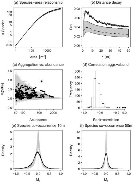
Testing the ability of a model that quantitatively fits the three rules to predict four additional patterns not used for parameter estimation. Predictions were derived with the model version including species‐specific dispersal and the field data is from the Barro Colorado Island (BCI) forest plot. The panels at the top show the species–area relationship (a) and the distance decay of community similarity (b). The latter is estimated by the probability F(r) that two trees separated by distance r belong to the same species. The dashed line and the grey area represent mean and 95% simulation envelopes for the model predictions using the 1000 best parameter sets. The black solid lines show the six BCI censuses (1985–2010). Panel (c) shows the relationship between species aggregation indices M _i(r) at the scale of 50 m versus species abundances. Panel (d) shows the distribution of Spearman rank‐correlation coefficients for the relationship between M_i(50 m) and species abundances. In panels (c) and (d) the grey points and the histogram show simulation results, while the black points show results for the six BCI censuses. The bottom row shows the distribution of spatial co‐occurrence indices M _ij(r) for species pairs at the scales of 10 m (e) and 50 m (f). The grey lines show the model predictions and the black solid lines the six BCI censuses. The vertical dashed line indicates the expectation for spatially independent species distributions. See the main text for the interpretation of the spatial co‐occurrence index M _ij(r).

The distributions of co‐occurrence patterns of species pairs showed a similar shape in the model predictions and in the field data, but the observed distribution was somewhat wider, indicating larger variability in the field than in the model (Fig. 3e,f). A closer look revealed that the model slightly overestimated the number of species pairs that showed an independent co‐occurrence pattern, while species pairs in the field showed stronger segregation (M_ij < 0) or stronger attraction (M_ij > 0) compared with the model predictions. These findings were consistent at the 10‐m and the 50‐m scales (Fig. 3e,f).

Question 3: Does the pattern fit differ between the two contrasting tropical forests?

For the forest plot in Sinharaja we found qualitatively the same results for model–data agreement and model–data mismatch as with the BCI data (see Figs A8–A10). However, the predicted distributions of pairwise co‐occurrence patterns at Sinharaja showed more pronounced differences from the observed distributions than for the BCI plot (compare Fig. 3e,f with Fig. A9e,f). This is in agreement with a previous static spatial analysis (Wiegand et al., 2012). The model clearly overestimated the proportion of species with indices M_ij(r) close to zero (i.e. independence) and underestimated the proportion of species that tended to show segregation or positive associations. The reason for this is probably the strong topographic heterogeneity at the Sinharaja plot (Wiegand et al., 2012; Punchi‐Manage et al., 2013) that causes species with shared habitat associations to be more positively associated (than expected by a homogeneous model) and species with opposed habitat associations to be more segregated. For the abundance distribution we found minor deviations in Sinharaja in the number of tree species represented by just one individual (Fig. A8a) which might be related to uncertainty in species taxonomy.

Discussion

In this study we investigated the intriguing question raised by McGill (2010) of whether a minimal set of rules exists that specifies the stochastic spatial geometry of biodiversity. Existence of such a minimal set would indicate that we have achieved a useful description of the rules governing species abundances, diversity and distributions. We used simulations of simple dynamic and spatially explicit forest community models, embedded within a framework of inverse modelling, to transform the qualitative rules of McGill (2010) (e.g. a ‘hollow‐curve’ SAD) into model parameterizations that quantitatively match the observed biodiversity patterns found in two tropical forest plots. In a second step we tested if the model that was parameterized to fit the three rules correctly also predicts four additional observed biodiversity patterns without additional calibration.

Our analyses provided clear answers to our three guiding questions. First, we found that predicting the observed distribution of species aggregation requires species‐specific dispersal distances. Second, matching the three minimal sufficient rules resulted in correct predictions of the SAR but did not ensure realistic predictions of other spatial biodiversity patterns, including the distance decay, the relationship between species abundances and aggregation and the distribution of species co‐occurrences. Third, the ability of the extended model to predict multiple spatial biodiversity patterns in the two contrasting forests was surprisingly similar, except that species co‐occurrence predictions were poorer for the Sinharaja forest plot that has a stronger topographic structure.

Predictions of the three minimal rules and of additional spatial biodiversity patterns

The finding that species‐specific dispersal kernels were needed to approximate the observed distribution of intraspecific aggregation does not come as a surprise. Several studies that have conducted point‐pattern analyses of species distributions found substantial differences among species cluster sizes (e.g. Condit et al., 2000) that could at least partly be related to the species dispersal syndrome (Seidler & Plotkin, 2006). Additionally, spatial analyses that extended the Poisson‐cluster approach showed that species‐specific aggregation is needed to match the SAR and the distance decay (Shen et al., 2009; Wang et al., 2011).

Our finding that the SAR can be predicted based on the SAD and intraspecific aggregation is in good agreement with previous studies using spatially explicit models (Horvat et al., 2010) or spatial point‐pattern analysis (Plotkin et al., 2000). He & Legendre (2002) even derived analytical expressions for the SAR based on species abundances and their aggregation. Furthermore, Condit et al. (2002) found that a spatially explicit neutral model predicts a realistic distance decay at intermediate scales but fails at short scales (e.g. within forest plots) and at very large spatial scales. This is also in line with our result that the three rules are insufficient to predict the SAR and the distance decay simultaneously (May et al., 2015).

In contrast to our findings, studies using static Poisson‐cluster models correctly predicted the SAR and the distance decay simultaneously, at least in forests with a relatively homogeneous environment (Morlon et al., 2008; Wang et al., 2011, 2015). The interesting question is why the purely phenomenological Poisson‐cluster models successfully predicted SAR and distance decay simultaneously, while our mechanistic and dynamic model, which also considers abundances and intraspecific aggregation, failed in the simultaneous prediction. Equation (2) suggests that a positive correlation between abundance (f_i) and aggregation (g_i(r)) will produce large values of F(r) for a fixed distance r, whereas a negative relationship will produce low values. (Note that the g(r) is not strongly influenced by the abundance‐aggregation relationship.) The important point is therefore that static Poisson‐cluster models impose the observed relationship between species abundances and species aggregation. These descriptive models, however, do not provide any mechanistic explanation for observed abundance–aggregation relationships that would be based on biological processes. In contrast our model does not a priori constrain the relationship between relative abundances f_i and species aggregations g_i(r), but this relationship dynamically emerges from the processes of dispersal and ecological drift. In this way the failure of the dynamic model to correctly predict SAR and distance decay simultaneously provides important information. It highlights that we still lack a mechanistic understanding of observed abundance–aggregation relationships and suggests that this relationship might be considered as a ‘hidden fourth rule’ that has been lacking in previous unified theories of biodiversity.

Lessons from our study

Overall our study demonstrates that the three rules advocated by McGill (2010) provide only an incomplete approximation of the stochastic geometry of biodiversity and do not necessarily provide realistic predictions of multiple macroecological biodiversity patterns. This failure raises the question of whether these rules are in principle correct, but need to be extended by additional rules, or if they include unrealistic assumptions that need to be adapted to enable an improved understanding and better predictions of multiple biodiversity patterns.

The mismatch between model predictions and field observations in the distribution of the co‐occurrence of species pairs (Figs 3e,f & A9e,f) is likely to indicate deviations from the assumption of independent interspecific placement (rule 3). In general, deviations from spatial independence can either result from habitat preferences or species interactions, where species interactions typically influence co‐occurrence patterns at the direct neighbourhood scale but habitat association at larger scales (Wiegand et al., 2012). Species with similar habitat preferences will therefore show positive values of M_ij(r) because they tend to co‐occur at the spatial scales imposed by the habitat structure, while species with distinct habitat requirements will show negative values of M_ij(r) (Wiegand et al., 2007). In a similar way species that facilitate each other will at smaller scales show attraction (M_ij(r) > 1) and species which compete intensively for space or resources will show small‐scale segregation (M_ij(r) < 1).

We hypothesize that habitat preferences, but not biotic interactions, are the main reason for the failure of our models to predict the interspecific co‐occurrence patterns in the tropical forest plots studied here. First, previous studies found evidence for significant habitat associations of several species in the two forest plots (e.g. Harms et al., 2001; Kanagaraj et al., 2011; Punchi‐Manage et al., 2013), which also indicated stronger habitat association patterns in the Sinharaja forest compared with the BCI forest. This finding matches well with our finding that departures from the interspecific co‐occurrence patterns were larger for Sinharaja than for BCI. Second, Wiegand et al. (2012) found in an analysis of species segregation versus species mixing that spatial patterns at relatively large scales were likely to be driven by habitat preference. In contrast, in a subsequent analysis of species co‐occurrence at short distances (r < 30 m), which controlled for the effect of habitat associations, only a few species pairs showed departures from independence. The latter result might indicate that pairwise competitive or facilitative tree interactions at short distances do not strongly affect the co‐distribution of species pairs in the tropical forests studied. However, we expect that pairwise species interactions are more important in species‐poorer temperate forests (e.g. Wiegand et al., 2012) in producing non‐independent interspecific co‐occurrence patterns. Interactions include, for example, priority effects and succession which make certain species combinations more (or less) likely to spatially co‐occur.

Our model included the assumption that all species share the same mortality rate of c. 2%. This is clearly a simplification of reality and was included to foster model parameterization and understanding. However, this simplification is supported by an extensive study which found no clear relationship between species diversity and interspecific variation in mortality and recruitment rates (Condit et al., 2006). In contrast to expectations of niche theory, the most diverse forests even featured the lowest interspecific variation in demographic rates. These findings provide some evidence that interspecific variation in mortality and recruitment is unlikely to be a major driver of macroecological biodiversity patterns.

Our model failed to reproduce realistic abundance–aggregation relationships, although the marginal distributions of species abundances and aggregations were predicted correctly. In the model we obtained too many rare and aggregated species, and in the data we found more aggregated and abundant species than predicted by the model. This finding raises the question of which processes remove or obscure a correlation between aggregation and abundances in real forests? Certainly, several non‐mutually exclusive mechanisms are responsible for this. For example, aggregation of common species may be related to habitat associations. The question of why some rare species are widely distributed is more difficult to answer. One possibility is that some rare and widely dispersed species have a specific dispersal vector, for example animals with long travel distances, which fosters high dispersion of trees (Seidler & Plotkin, 2006; Muller‐Landau et al., 2008). Another explanation might be offered by negative conspecific density dependence (Comita et al., 2010). Strong negative effects of conspecific neighbours (e.g. by species‐specific herbivores or pathogens) in rare species might result in less aggregated patterns.

Conclusions

We asked here if a minimal set of rules exists that yields a reasonable approximation of a predefined set of biodiversity patterns that are regarded as important indicators of the stochastic geometry of biodiversity. Our study indicates that the rules of McGill (2010) provided a good starting point, but that they need to be adapted and extended to provide quantitative predictions of the four additional spatial biodiversity patterns selected. Our findings suggest that rule 3 (interspecific independence) should be relaxed by incorporating species‐specific habitat associations to better quantify co‐occurrence and segregation of species, as well as aggregation of common species. Further analyses are required to clarify the role of correlations between species‐specific dispersal distances, negative density dependence and species abundances. These three factors – habitat, dispersal and density dependence – can all influence species aggregation and we showed that knowledge about abundance–aggregation relationships is important for a quantitative prediction of the distance decay function.

Overall, it is unlikely that we will ever find a small set of sufficient rules that will govern every possible pattern in the complex stochastic spatial geometry of biodiversity. Clearly, the more detail and site‐specific idiosyncrasies that the model needs to fit the more detail we need to include. It is therefore important to define a priori the desired level of detail, i.e. which patterns we wish to match with a certain approach. The results presented here are encouraging and suggest that we may indeed find a limited set of key rules that can result in a good approximation of major biodiversity patterns of ecological communities and explain the fundamental axes of variation among communities. Stepwise extension of current biodiversity theories and the quantitative confrontation of their predictions with field data, as outlined in this study, provides an exciting and promising research agenda for improving our understanding of biodiversity in space and time.

Biosketch.

The involved authors are researchers within the European Research Council (ERC) ERC‐funded research project ‘Spatiodiversity’ (http://www.thorsten‐wiegand.de/towi_ERC.html) that aims to understand the relative importance of processes and factors that govern the composition and dynamics of species‐rich communities. The project integrates information on spatial patterns, which are buried in stem‐mapped forests, with dynamic and spatially explicit forest models and statistical inference for stochastic simulation models.

Supporting information

Appendix S1 Detailed description of the CONFETTI model and the parameter estimation approach.

Appendix S2 Supplementary figures on parameter estimates and model predictions.

Appendix S3 Point pattern theory and the link between the distance decay, species abundance and aggregation.

References

- Ashton, P.S. (1964) Ecological studies in the mixed dipterocarp forests of Brunei State. Clarendon Press, Oxford. [Google Scholar]
- Beaumont, M.A. (2010) Approximate Bayesian computation in evolution and ecology. Annual Review of Ecology, Evolution, and Systematics, 41, 379–406. [Google Scholar]
- Brown, J.H. , Mehlman, D.W. & Stevens, G.C. (1995) Spatial variation in abundance. Ecology, 76, 2028–2043. [Google Scholar]
- Chase, J.M. (2005) Towards a really unified theory for metacommunities. Functional Ecology, 19, 182–186. [Google Scholar]
- Chave, J. & Leigh, E.G. (2002) A spatially explicit neutral model of β‐diversity in tropical forests. Theoretical Population Biology, 62, 153–168. [DOI] [PubMed] [Google Scholar]
- Chave, J. , Muller‐Landau, H.C. & Levin, S.A. (2002) Comparing classical community models: theoretical consequences for patterns of diversity. The American Naturalist, 159, 1–23. [DOI] [PubMed] [Google Scholar]
- Comita, L. , Muller‐Landau, H. , Aguilar, S. & Hubbell, S. (2010) Asymmetric density dependence shapes species abundances in a tropical tree community. Science, 329, 330–332. [DOI] [PubMed] [Google Scholar]
- Condit, R. (1998) Tropical forest census plots. Springer, Berlin. [Google Scholar]
- Condit, R. , Ashton, P.S. , Baker, P. , Bunyavejchewin, S. , Gunatilleke, S. , Gunatilleke, N. , Hubbell, S.P. , Foster, R.B. , Itoh, A. , Lafrankie, J.V. , Lee, H.S. , Losos, E. , Manokaran, N. , Sukumar, R. & Yamakura, T. (2000) Spatial patterns in the distribution of tropical tree species. Science, 288, 1414–1418. [DOI] [PubMed] [Google Scholar]
- Condit, R. , Pitman, N. , Leigh, E.G. , Chave, J. , Terborgh, J. , Foster, R.B. , Nunez, P. , Aguilar, S. , Valencia, R. , Villa, G. , Muller‐Landau, H.C. , Losos, E. & Hubbell, S.P. (2002) Beta‐diversity in tropical forest trees. Science, 295, 666–669. [DOI] [PubMed] [Google Scholar]
- Condit, R. , Ashton, P. , Bunyavejchewin, S. et al (2006) The importance of demographic niches to tree diversity. Science, 313, 98–101. [DOI] [PubMed] [Google Scholar]
- Etienne, R.S. & Alonso, D. (2005) A dispersal‐limited sampling theory for species and alleles. Ecology Letters, 8, 1147–1156. [DOI] [PubMed] [Google Scholar]
- Greene, D.F. , Canham, C.D. , Coates, K.D. & Lepage, P.T. (2004) An evaluation of alternative dispersal functions for trees. Journal of Ecology, 92, 758–766. [Google Scholar]
- Grimm, V. , Revilla, E. , Berger, U. , Jeltsch, F. , Mooij, W.M. , Railsback, S.F. , Thulke, H.‐H. , Weiner, J. , Wiegand, T. & DeAngelis, D.L. (2005) Pattern‐oriented modeling of agent‐based complex systems: lessons from ecology. Science, 310, 987–991. [DOI] [PubMed] [Google Scholar]
- Gunatilleke, C.V.S. , Gunatilleke, I.A.U.N. , Ashton, P.S. , Ethugala, A.U.K. , Weerasekara, N.S. & Esufali, S. (2004a) Sinharaja forest dynamics plot, Sri Lanka Tropical forest diversity and dynamism. Findings from a large‐scale plot network (ed. by Losos E.C. and Leigh E.G.), pp. 599–608. University of Chicago Press, Chicago, IL. [Google Scholar]
- Gunatilleke, C.V.S. , Gunatilleke, I.A.U.N. , Ethugala, A.U.K. & Esufali, S. (2004b) Ecology of Sinharaja rain forest and the forest dynamics plot in Sri Lanka's natural world heritage site. WHT Publications, Colombo. [Google Scholar]
- Gunatilleke, C.V.S. , Gunatilleke, I.A.U.N. , Esufali, S. , Harms, K.E. , Ashton, P.M.S. , Burslem, D.F.R.P. & Ashton, P.S. (2006) Species–habitat associations in a Sri Lankan dipterocarp forest. Journal of Tropical Ecology, 22, 371–384. [Google Scholar]
- Harms, K.E. , Condit, R. , Hubbell, S.P. & Foster, R.B. (2001) Habitat associations of trees and shrubs in a 50‐ha Neotropical forest plot. Journal of Ecology, 89, 947–959. [Google Scholar]
- Harte, J. , Zillio, T. , Conlisk, E. & Smith, A.B. (2008) Maximum entropy and the state‐variable approach to macroecology. Ecology, 89, 2700–2711. [DOI] [PubMed] [Google Scholar]
- Hartig, F. , Calabrese, J.M. , Reineking, B. , Wiegand, T. & Huth, A. (2011) Statistical inference for stochastic simulation models – theory and application. Ecology Letters, 14, 816–827. [DOI] [PubMed] [Google Scholar]
- He, F. & Legendre, P. (2002) Species diversity patterns derived from species–area models. Ecology, 83, 1185–1198. [Google Scholar]
- He, F. , Legendre, P. & LaFrankie, J.V. (1997) Distribution patterns of tree species in a Malaysian tropical forest. Journal of Vegetation Science, 8, 105–114. [Google Scholar]
- Horvat, S. , Derzsi, A. , Neda, Z. & Balog, A. (2010) A spatially explicit model for tropical tree diversity patterns. Journal of Theoretical Biology, 265, 517–523. [DOI] [PubMed] [Google Scholar]
- Hubbell, S.P. (2001) The unified neutral theory of biodiversity and biogeography. Princeton University Press, Princeton, NJ. [DOI] [PubMed] [Google Scholar]
- Hubbell, S.P. , Foster, R.B. , O'Brien, S.T. , Harms, K.E. , Condit, R. , Wechsler, B. , Wright, S.J. & de Lao, S.L. (1999) Light‐gap disturbances, recruitment limitation, and tree diversity in a Neotropical forest. Science, 283, 554–557. [DOI] [PubMed] [Google Scholar]
- Hubbell, S.P. , Condit, R. & Foster, R.B. (2005) Barro Colorado forest census plot data. Available at: http://ctfs.arnarb.harvard.edu/webatlas/datasets/bci (accessed 17 June 2014).
- Jabot, F. & Chave, J. (2009) Inferring the parameters of the neutral theory of biodiversity using phylogenetic information and implications for tropical forests. Ecology Letters, 12, 239–248. [DOI] [PubMed] [Google Scholar]
- Kanagaraj, R. , Wiegand, T. , Comita, L.S. & Huth, A. (2011) Tropical tree species assemblages in topographical habitats change in time and with life stage. Journal of Ecology, 99, 1441–1452. [Google Scholar]
- Lehmann, S. & Huth, A. (2015) Fast calibration of a dynamic vegetation model with minimum observation data. Ecological Modelling, 301, 98–105. [Google Scholar]
- McGill, B.J. (2010) Towards a unification of unified theories of biodiversity. Ecology Letters, 13, 627–642. [DOI] [PubMed] [Google Scholar]
- McGill, B.J. , Etienne, R.S. , Gray, J.S. , Alonso, D. , Anderson, M.J. , Benecha, H.K. , Dornelas, M. , Enquist, B.J. , Green, J.L. , He, F.L. , Hurlbert, A.H. , Magurran, A.E. , Marquet, P.A. , Maurer, B.A. , Ostling, A. , Soykan, C.U. , Ugland, K.I. & White, E.P. (2007) Species abundance distributions: moving beyond single prediction theories to integration within an ecological framework. Ecology Letters, 10, 995–1015. [DOI] [PubMed] [Google Scholar]
- May, F. , Giladi, I. , Ziv, Y. & Jeltsch, F. (2012) Dispersal and diversity – unifying scale‐dependent relationships within the neutral theory. Oikos, 121, 942–951. [Google Scholar]
- May, F. , Huth, A. & Wiegand, T. (2015) Moving beyond abundance distributions: neutral theory and spatial patterns in a tropical forest. Proceedings of the Royal Society B: Biological Sciences, 282, 20141657. [DOI] [PMC free article] [PubMed] [Google Scholar]
- Morlon, H. , Chuyong, G. , Condit, R. , Hubbell, S. , Kenfack, D. , Thomas, D. , Valencia, R. & Green, J.L. (2008) A general framework for the distance‐decay of similarity in ecological communities. Ecology Letters, 11, 904–917. [DOI] [PMC free article] [PubMed] [Google Scholar]
- Muller‐Landau, H.C. , Wright, S.J. , Calderon, O. , Condit, R. & Hubbell, S.P. (2008) Interspecific variation in primary seed dispersal in a tropical forest. Journal of Ecology, 96, 653–667. [Google Scholar]
- Plotkin, J.B. , Potts, M.D. , Leslie, N. , Manokaran, N. , LaFrankie, J. & Ashton, P.S. (2000) Species–area curves, spatial aggregation, and habitat specialization in tropical forests. Journal of Theoretical Biology, 207, 81–99. [DOI] [PubMed] [Google Scholar]
- Punchi‐Manage, R. , Getzin, S. , Wiegand, T. , Kanagaraj, R. , Gunatilleke, C.V.S. , Gunatilleke, I.A.U.N. , Wiegand, K. & Huth, A. (2013) Effects of topography on structuring local species assemblages in a Sri Lankan mixed dipterocarp forest. Journal of Ecology, 101, 149–160. [DOI] [PubMed] [Google Scholar]
- Rosenzweig, M.L. (1995) Species diversity in space and time. Cambridge University Press, Cambridge. [Google Scholar]
- Rosindell, J. & Cornell, S.J. (2009) Species–area curves, neutral models, and long‐distance dispersal. Ecology, 90, 1743–1750. [DOI] [PubMed] [Google Scholar]
- Seidler, T.G. & Plotkin, J.B. (2006) Seed dispersal and spatial pattern in tropical trees. PLoS Biology, 4, 2132–2137. [DOI] [PMC free article] [PubMed] [Google Scholar]
- Shen, G.C. , Yu, M.J. , Hu, X.S. , Mi, X.C. , Ren, H.B. , Sun, I.F. & Ma, K.P. (2009) Species–area relationships explained by the joint effects of dispersal limitation and habitat heterogeneity. Ecology, 90, 3033–3041. [DOI] [PubMed] [Google Scholar]
- Volkov, I. , Banavar, J. , Hubbell, S. & Maritan, A. (2007) Patterns of relative species abundance in rainforests and coral reefs. Nature, 450, 45–49. [DOI] [PubMed] [Google Scholar]
- Wang, X. , Wiegand, T. , Wolf, A. , Howe, R. , Davies, S.J. & Hao, Z. (2011) Spatial patterns of tree species richness in two temperate forests. Journal of Ecology, 99, 1382–1393. [Google Scholar]
- Wang, X. , Wiegand, T. , Swenson, N.G. , Wolf, A.T. , Howe, R.W. , Hao, Z. , Lin, F. , Ye, J. & Yuan, Z. (2015) Mechanisms underlying local functional and phylogenetic beta diversity in two temperate forests. Ecology, 96, 1062–1073. [DOI] [PubMed] [Google Scholar]
- Whitmore, T.C. (1984) Tropical rain forests of the far East. Oxford University Press, Oxford. [Google Scholar]
- Wiegand, T. & Moloney, K.A. (2014) Handbook of spatial point‐pattern analysis in ecology. CRC Press, Boca Raton, FL. [Google Scholar]
- Wiegand, T. , Jeltsch, F. , Hanski, I. & Grimm, V. (2003) Using pattern‐oriented modeling for revealing hidden information: a key for reconciling ecological theory and application. Oikos, 100, 209–222. [Google Scholar]
- Wiegand, T. , Gunatilleke, C.V.S. & Gunatilleke, I.A.U.N. (2007) Species associations in a heterogeneous Sri Lankan dipterocarp forest. The American Naturalist, 170, E77–E95. [DOI] [PubMed] [Google Scholar]
- Wiegand, T. , Huth, A. , Getzin, S. , Wang, X. , Hao, Z. , Gunatilleke, S. & Gunatilleke, N. (2012) Testing the independent species' arrangement assertion made by theories of stochastic geometry of biodiversity. Proceedings of the Royal Society B: Biological Sciences, 279, 3312–3320. [DOI] [PMC free article] [PubMed] [Google Scholar]
- Zhang, J. & Sanderson, A.C. (2009) JADE: adaptive differential evolution with optional external archive. IEEE Transactions on Evolutionary Computation, 13, 945–958. [Google Scholar]
Associated Data
This section collects any data citations, data availability statements, or supplementary materials included in this article.
Supplementary Materials