MIDAS robust trend estimator for accurate GPS station velocities without step detection

Abstract

Automatic estimation of velocities from GPS coordinate time series is becoming required to cope with the exponentially increasing flood of available data, but problems detectable to the human eye are often overlooked. This motivates us to find an automatic and accurate estimator of trend that is resistant to common problems such as step discontinuities, outliers, seasonality, skewness, and heteroscedasticity. Developed here, Median Interannual Difference Adjusted for Skewness (MIDAS) is a variant of the Theil‐Sen median trend estimator, for which the ordinary version is the median of slopes v_ij = (x_j–x_i)/(t_j–t_i) computed between all data pairs i > j. For normally distributed data, Theil‐Sen and least squares trend estimates are statistically identical, but unlike least squares, Theil‐Sen is resistant to undetected data problems. To mitigate both seasonality and step discontinuities, MIDAS selects data pairs separated by 1 year. This condition is relaxed for time series with gaps so that all data are used. Slopes from data pairs spanning a step function produce one‐sided outliers that can bias the median. To reduce bias, MIDAS removes outliers and recomputes the median. MIDAS also computes a robust and realistic estimate of trend uncertainty. Statistical tests using GPS data in the rigid North American plate interior show ±0.23 mm/yr root‐mean‐square (RMS) accuracy in horizontal velocity. In blind tests using synthetic data, MIDAS velocities have an RMS accuracy of ±0.33 mm/yr horizontal, ±1.1 mm/yr up, with a 5th percentile range smaller than all 20 automatic estimators tested. Considering its general nature, MIDAS has the potential for broader application in the geosciences.

Key Points

• MIDAS is a robust estimator of time series trend

• MIDAS estimates of GPS velocities are resistant to outliers, steps, and seasonality

• MIDAS velocities are as accurate as the best methods involving step detection

1. Introduction

1.1. Motivation

Accurate station velocities are needed for many geodetic investigations in geophysics, including plate tectonics, strain across faults systems, the contribution of vertical land motion to regional sea level, glacial isostatic adjustment, mountain uplift, subsidence, and secular unloading/loading of water reservoirs and ice sheets. To illustrate the magnitude of the problem, the recent global tectonic model of Kreemer et al. [2014] required the time‐consuming, manual screening of the east and north component time series from over 6700 stations.

In addition, for the case where a geophysical event such as an earthquake or the onset of volcanic activity may have recently displaced a station, it is useful to determine the preevent velocity as a reference velocity to detrend the coordinate time series. Doing this automatically would facilitate rapid event analysis and could even be used to issue an alert for potential events that may otherwise go undetected.

All of the above motivates us to find a way to estimate station velocities accurately without the need for manual screening. Such velocity estimates should be resistant to the kinds of problems we shall now explore that are common in GPS time series. Moreover, the velocity estimates should each come with a realistic uncertainty computed using robust statistics of dispersion.

1.2. Common Problems

A common problem in GPS time series is seasonality. The presence of seasonal signals can significantly bias velocity estimates unless they are mitigated. This is particularly problematic for shorter time series in least squares analysis owing to correlations between velocity and seasonal parameters [Blewitt and Lavallée, 2002].

Much of the literature on statistics of errors in geodetic time series has given appropriate attention to spectral characterization [e.g., Williams et al., 2004]. Yet expert analysts know intuitively that many of the specific error sources in time series require some degree of characterization in the time domain [Agnew, 1992]. One common example is the presence of step discontinuities in the time series caused by equipment changes, which not reflect geophysical motion of a station. In this case, the estimated velocity should reflect the trends between the steps, as if the steps were absent [Williams, 2003]. In the case of least squares analysis, steps can be estimated simultaneously with velocity but, unless the step epochs are known, some kind of step detection algorithm needs to be applied first. Yet to date, blind tests conducted on detecting step discontinuities in GPS data prove that the best expert eyeball performs better than the world's best automatic methods [Gazeaux et al., 2013].

Other common time domain problems in GPS data include outliers, time‐dependent noise (heteroscedasticity), and unmodeled events in general. For example, it is typically the case that the noise level in GPS time series tends to be worse for earlier data, when there were fewer satellites and reference frame stations. Such heteroscedasticity may not be accurately characterized by formal errors. As another example, GPS time series tend to be noisier in summer than winter, because of increased variation in atmospheric refractivity [Blewitt et al., 2013]. However, some stations that are subject to sustained snow cover may experience the opposite seasonal effect.

The eyeball is good at discerning temporal patterns of errors like these that can be harmful to least squares estimation. There are also problems in GPS time series with nonnormal probability distribution functions (PDF) that can be obvious to the eye but are not handled well by traditional methods that involve a combination of least squares estimation with outlier and step detection. Examples of pathological features include skewness (asymmetric PDF), kurtosis (sharp‐peaked, long‐tailed PDF), and multiple peaks (multimodal PDF).

1.3. Current Approach

Operational methods to date, whether automatic or not, typically iterate on two broad steps: (1) apply least squares estimation to coordinate time series according to a parametric model that at least includes station velocity and Fourier coefficients to fit seasonal signals and (2) attempt to detect and remove outliers or problematic periods of data, detect step discontinuities, and insert extra parameters to estimate each detected step. A problem with this approach is that the initial least squares fit is biased, thus impacting the detection of steps [Gazeaux et al., 2013]. Iteration may not always solve this problem satisfactorily.

Such types of algorithms that require step detection can fail in two possible ways. On the one hand, failing to detect real permanent steps will bias the estimates of station velocity and other possible parameters. On the other hand, the detection of false positives can lead to unnecessary degradation of precision in the determination of station velocity, with negative impact on the stability of reference frames realized from such data [Blewitt et al., 2013].

1.4. MIDAS Approach

Least squares estimation predominates in geodesy; indeed, it has been argued that least squares was invented for geodesy by Gauss [Stigler, 1981]. The almost complete dependence of geodetic practice on least squares estimation is hard to justify considering that least squares (alone) is not robust and that a large body of research has revolutionized robust estimation theory and practice over the last few decades [Wilcox, 2005].

This paper develops a robust median trend estimator based on Theil‐Sen [Theil, 1950; Sen, 1968], which is well known and used in many fields of science such as astronomy [Akritas et al., 1995], remote sensing [Fernandes and Leblanc, 2005], and hydrology [Helsel and Hirsch, 2002]. The ordinary version of Theil‐Sen works by taking the median trend (50th percentile) between all possible pairs of data. Thus, outliers have negligible effect, and the result reflects the predominant relationship between points, which the eye naturally detects.

Median Interannual Difference Adjusted for Skewness (MIDAS) is a customized version of Theil‐Sen that incorporates the qualities needed for accurate GPS station velocity estimation, such as insensitivity to seasonal variation. MIDAS has features designed to make trend estimates resistant to step discontinuities in the time series. Figure 1 uses a simple example of simulated data to provide an intuitive impression of the insensitivity of MIDAS velocity estimates to steps that can be barely detected by eye. Figure 1 also shows what happens to least squares estimates if step detection fails. In addition, MIDAS computes a realistic velocity uncertainty that is based on the observed distribution of sampled slopes.

Figure 1.

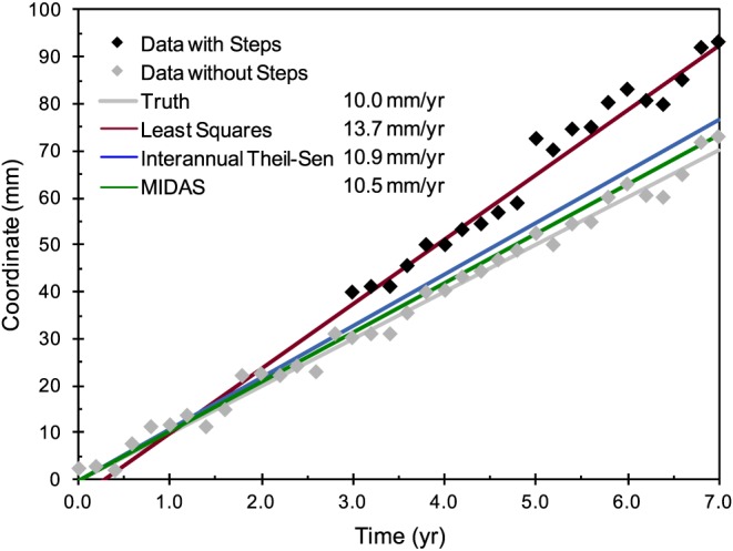
Example of simulated time series with steps, showing trends estimated by least squares (maroon), interannual Theil‐Sen (blue), and MIDAS (green). None of the estimators model the steps. To visualize how well each estimator fits the data, also plotted are data without steps and the true trend (gray). Steps of 10 mm are added at 3.0 year and 5.0 year. The simulated data include an annual sinusoidal signal of amplitude 2 mm and random errors with standard deviation 1.5 mm. Least squares simply fails without step parameters. The MIDAS trend error is 0.5 ± 0.5 mm/yr, reducing the bias in the interannual Theil‐Sen by 50%.

After developing and testing the methodology, this paper concludes with a summary of our findings and our thoughts on the applicability of the MIDAS method for automation in GPS geodesy and in other disciplines. Appendix A provides a theoretical derivation of statistics that rigorously quantify the robustness of MIDAS to outliers and steps.

2. Methodology

2.1. The Ordinary Theil‐Sen Estimator

The development of the MIDAS estimator starts by considering the ordinary Theil‐Sen estimator, which for the case of coordinate time series is defined as the median of slopes between pairs of data:

$$\widehat{v}={\text{median}}_{j>i}\left(\frac{x_j-x_i}{t_j-t_i}\right)$$ (1)

where coordinate x_i is sampled at time t_i.

The ordinary version of Theil‐Sen computes the median slope between all possible pairs of a coordinate time series. In the development of MIDAS that follows below, we modify the selection of pairs in order to reduce sensitivity to seasonality and step discontinuities.

Conventionally, the median slope is defined by ranking the slopes of the selected n data pairs from lowest to highest values: v(p − 1) < v(p). The median can then be defined as middle ranking value if n is odd; if n is even, the median is the average of the two middle values:

$$\widehat{v}={\text{median}}_p\left[v\left(p\right)\right]=\left\{\begin{array}{r}\hfill v\left[\left(n+1\right)/2\right],\mathrm{f}\mathrm{o}\mathrm{r}\text{odd}n\\ \hfill \frac{v\left(n/2\right)+v\left(n/2+1\right)}{2},\mathrm{f}\mathrm{o}\mathrm{r}\text{even}n\end{array}\right.$$ (2)

It turns out that computing the median does not actually require sorting all the data, which can be computationally expensive. Instead, we use the “quickselect” algorithm by Hoare [1961], which can find any specified percentile in a computation time that, in practice, scales linearly with the number of data O(n).

2.2. The Interannual Theil‐Sen Estimator

To mitigate seasonality, researchers in water resources [e.g., Hirsch et al., 1982; Helsel and Hirsch, 2002] suggest selecting only data that are separated by an integer number of years. An important feature of our procedure is that we restrict this selection even further by demanding that data pairs be separated by just 1 year, which makes the estimator less sensitive to step discontinuities. Pairs of data spanning a step discontinuity will produce velocity samples that are on one of the tails of the distribution. Demanding that the time separation be just 1 year rather than any integer year minimizes the fraction of pairs that span discontinuities while maintaining insensitivity to seasonality.

It is common for time series to have time specified by real‐valued years, for which 1 day is defined as 1/365.25 years. In this case, to select a single pair it is sufficient to require

$$0.999\text{year}<\left(t_j-t_i\right)<1.001\text{year}$$ (3)

for which the pair will be separated by 365 days. Clearly, the specific choice of 365 days could be relaxed to some degree while preserving insensitivity to seasonality. It might be thought that allowing all possible pairs within a wider time window around 1 year might generate superior results. We tested this idea by gradually widening the window up to 100 days wide to allow up to 10⁴ more pairs. We found that the velocity estimates change very little at the ~0.1 mm/yr level. This suggests that our minimal selection of pairs contains essentially all of the independent information available. A big advantage of this approach is that the number of computations is reduced by orders of magnitude, as the number of pairs for our selection method goes linearly with the number of data O(n).

2.3. The MIDAS Estimator

If step discontinuities exist in the time series, the interannual Theil‐Sen trend estimate can be biased, because a step can produce a multimodal distribution of slopes from up to 365 data pairs spanning the step. Steps smaller than 2 standard deviations of the data noise will generally produce a unimodal distribution that is skewed (with one tail more populated than the other).

To handle this problem, we compute an initial value of the median trend using slopes from all selected data pairs and then define slopes as outliers (possibly associated with steps) if they are greater than 2 standard deviations on either side of the median. This requires an estimate of the standard deviation of the distribution that is not sensitive to outliers [Leys et al., 2013]. For this, we base our estimate on a well‐known robust estimator of dispersion known as the median of absolute deviations (MAD). The standard deviation can then be estimated robustly by scaling the MAD according to Wilcox [2005]:

$$\begin{array}{c}\text{MAD}={\text{median}}_p\left|v\left(p\right)-\widehat{v}\right|\\ \mathrm{\sigma }=1.4826\text{MAD}\end{array}$$ (4)

This estimate of standard deviation assumes that a majority of data reasonably fit a Gaussian PDF, with a minority of the data being outliers. Given this estimate of the standard deviation, final values of the median and standard deviation are computed after trimming the tails of the distribution beyond 2 standard deviations. The two steps can be summarized as follows:

$$\begin{array}{l}\text{Step}1\mathrm{:}\widehat{v}={\text{median}}_p\left|v\left(p\right)\right|\\ \sigma =1.4826{\text{median}}_p\left|v\left(p\right)-\widehat{v}\right|\\ \text{Step}2\mathrm{:}\text{Select}\left\{q=p\right\}\mathrm{f}\mathrm{o}\mathrm{r}\text{all}\left|v\left(p\right)-\widehat{v}\right|<2\sigma \\ \widehat{v}={\text{median}}_q\left|v\left(q\right)\right|\\ \sigma =1.4826{\text{median}}_q\left|v\left(q\right)-\widehat{v}\right|\end{array}$$ (5)

The specific choice of trimming tails beyond 2 standard deviations strikes a balance between having a small impact on a majority of data that has a Gaussian PDF while being effective at removing outliers arising from step discontinuities. Whereas the precise choice of 2 standard deviations is not important, simpler schemes based on trimming a specific percentage of both tails prove to be less effective because steps can introduce significant skewness to the distribution.

2.4. Relaxed Pair Selection

The selection of pairs of data 1 year apart works well for the case of continuous stations that produce station position estimates every day without gaps. At the opposite extreme, sporadic data from campaign stations may not have any pairs of data that satisfy this criterion. Somewhere between these extremes lie semicontinuous stations [Blewitt et al., 2009], which have campaign sessions that may last for months at a time, with large time gaps between the sessions. Since much valuable information lies in time series that have gaps, we are motivated to relax the selection criteria so that as much data as possible are used.

In designing the relaxed selection algorithm, we apply the following principles. (1) There should be negligible difference in estimates if we were to introduce small gaps in a time series. (2) The principle of time symmetry demands that if all the data were reversed in time, the magnitude of the velocity estimate should not change. (3) Selection should give first priority to pairs separated by 1 year. (4) A pair separated by more than 1 year must be selected if a 1 year pair cannot be formed.

We designed our code to satisfy all these principles.

1. There is no threshold that defines whether we treat a time series as continuous or otherwise. The same code applies to all time series.

2. The code runs the pair selection subroutine twice, firstly, in time order (“forward”) and secondly, in reverse time order (“backward”).

3. When moving forward or backward through the data to select pairs, the first priority is given to pairs 1 year apart, if they exist.

4. If there is no matching pair 1 year apart, the algorithm selects the next available data point that has not yet been matched. This prevents overdependence on specific data. If the points available for matching are exhausted because the end of the time series is reached, the search is reset to the closest matching pair at least 1 year apart.

The consequences of applying this relaxed algorithm are negligible for time series with a few short gaps. Generally, there is a large improvement for sporadic campaign time series, for which strict selection may fail to find any pairs at all. For time series with gaps, the relaxed algorithm adds significantly more slope samples to the distribution, resulting in a more precise estimate. On the other hand, the robustness of MIDAS for data with gaps is generally weaker than for continuous data, because there is more dependence on specific data (which may have problems) that are used multiple times. This motivates us to compute an uncertainty in velocity that realistically reflects the slope distribution and predicts catastrophic failure of the estimator.

2.5. Velocity Uncertainty

Using the iterated estimate for the standard deviation given in the second step of equation (5), the formal standard error in the median is estimated according to Kenney and Keeping [1954, p.212], under the assumption that the trimmed distribution is approximately normal:

$$\begin{array}{c}\widehat{\sigma }=\sqrt{\frac{\pi }{2}}\frac{\sigma }{\sqrt{N}}\\ \approx 1.2533\frac{\sigma }{\sqrt{N}}\end{array}$$ (6)

Recall that the estimate of the standard deviation is based on the MAD, equation (4), under the assumption that a majority of data have a Gaussian PDF, with a minority being outliers. This justifies the use of rules applicable to the normal distribution. Here N is the effective number of independent q slopes selected in step 2 of equation (5). We compute this by dividing the actual number by a factor 4 to account for the nominal number of times the original coordinate data are used to form pairs:

$$N=\frac{N_{\text{actual}}}{4}$$ (7)

Note that N will generally be different for each of the three coordinates of position, because of the way that tails are trimmed. As is common practice in GPS geodesy, we treat the time series in the east, north, and up component independently, as correlations between these components are typically small (~0.1). Moreover, systematic errors and step discontinuities tend to affect these components differently (e.g., antenna height change).

Finally, the MIDAS velocity uncertainty is defined as the scaled standard error in the median:

$$\widehat{s}=3\widehat{\sigma }$$ (8)

The scaling factor of 3 is chosen so that the error is realistically close to the root‐mean‐square (RMS) accuracy, according to tests using simulated data described later. The need for a scaling factor arises when data are autocorrelated, which also changes the effective number of independent observations [Zięba and Ramsa, 2011]. Autocorrelation can arise from power law noise [Agnew, 1992] such as flicker noise, which is pervasive in nature [Brody, 1969] and is therefore pervasive in GPS data [Williams et al., 2004].

2.6. Robustness

The robustness of an estimator can be quantified by its sample breakdown point, defined as the number of arbitrarily large outliers in a data set that can be tolerated before the estimate becomes arbitrarily large. The “asymptotic” breakdown point is defined for an infinite number of data. Least squares estimators, including the sample mean, have the worst possible asymptotic breakdown point of 0%. In contrast, the sample median has the best possible breakdown point of 50%. Even though the ordinary Theil‐Sen estimator is a median, it has a lower breakdown point of 1–2^−½ = 29%, because the fraction refers to the original data rather than the sampled pairs. This theoretical value is a direct consequence of Theil‐Sen sampling n(n–1)/2 pairs of data and is generally different for other sampling schemes.

The sample breakdown point of our interannual Theil‐Sen and MIDAS estimators are identical, but different than the ordinary Theil‐Sen. The MIDAS breakdown point for continuous time series is derived analytically in Appendix A. The asymptotic breakdown point is shown to be 0.25(1–1/T), where T is a dimensionless quantity defined as the time spanned by all the data divided by the time separation between data pairs (365 days). Therefore, up to 25% of data can be outliers for very long time series. This assumes the worst possible case where all bad coordinate data are paired with good data. Examples of the sample breakdown point are 10% at 1.25 years, 14% at 2.33 years, and 20% at 5 years. Other examples are shown in Table A1 of Appendix A. In the case of GPS time series, the fraction of outliers rarely exceeds a few percent if we discount the effect of step discontinuities (to be addressed next), so outliers are typically not problematic.

To quantify resistance to step discontinuities, we introduce the “step breakdown point,” defined as the minimum number of arbitrarily large steps that cause the estimator to give arbitrarily large values, as a function of the time span T in years. It is shown in Appendix A that the asymptotic step breakdown point for a continuous time series is (T–1)/2, rounded down to the nearest integer. No arbitrarily large steps can be tolerated until 3 years, after which one step can be tolerated. One more step can be tolerated for every 2 additional years. This assumes the worst possible case where steps do not overlap (are separated by more than 1 year) and where the steps are all in the same direction. Note that an infinite step in one direction would exactly cancel with a nonoverlapping step in the opposite direction, so it is possible to tolerate more steps than the step breakdown point.

In terms of breakdown point, the MAD and hence the MIDAS velocity uncertainty are just as robust as the velocity estimate. This is a desirable quality, because if the breakdown point is exceeded, the MAD can be arbitrarily large; thus, the MAD should appropriately reflect any catastrophic failure of the velocity estimate.

Finally, we point out that robustness can be enhanced if given a list of epochs at which steps may be expected due to known equipment changes or earthquakes. Our implementation of MIDAS has the option of reading such a list and using it to prevent the sampling of slopes from data pairs that span such epochs. This option was not exercised in any of the tests described here.

2.7. Limitations

Before discussing limitations of MIDAS, we first point out that other specific choices could have been made in the MIDAS algorithm that would yield similar results. We do not claim that MIDAS is theoretically optimal; rather, we emphasize the importance of its general design to be insensitive to common problems in GPS data, such as steps and seasonality. We also emphasize that the robustness and accuracy of MIDAS should in the end depend on testing using real and simulated data that exhibit common problems.

Like any estimator, MIDAS has its limitations, and users should exercise appropriate caution. First of all, if the station really does have a nonconstant velocity, then interpretation of the MIDAS velocity can be problematic. However, appropriate interpretation of the MIDAS velocity may be possible, depending on the situation. For example, in the case where the station was subject to an event that occurs after the midpoint of a time series, such as an earthquake followed by postseismic deformation, the MIDAS velocity can be interpreted as the preevent velocity. We emphasize that MIDAS is simply a trend estimator and that other estimators would need to be applied to study other factors influencing the time series. Nevertheless, it may be useful to subtract the preevent velocity estimated by MIDAS from the postevent time series to characterize the event‐induced signal.

Secondly, MIDAS does not mitigate the effects of periodic signals unless they are harmonics of 1 year. That is, MIDAS is completely insensitive to seasonal signals of any annually repeating form, but it could be sensitive to large periodic signals that do not repeat exactly from 1 year to the next, or signals of other frequency. Fortunately, the level of velocity bias caused by periodic signals averages down quickly with time, faster than that for white noise [Blewitt and Lavallée, 2002]. We investigated the specific case of a sinusoidal signal with the draconitic (eclipse) period of the GPS satellite constellation, which at ~351 days differs from 365 days because of precession of the orbit nodes [Griffiths and Ray, 2013]. We find by simulation that a 1 mm amplitude signal biases the MIDAS velocity within a negligible maximum range of ±0.03 mm/yr for time series spanning 2 to 3 years (and rapidly falling with each passing year).

Finally, the computation of breakdown point in this paper assumed a continuous time series; hence, the robustness of MIDAS cannot be guaranteed for time series with gaps. We have not attempted to quantify how the robustness of MIDAS degrades, as the time series becomes more sparse, because this problem is not tractable analytically. Even a Monte Carlo simulation would not address this question satisfactorily, because the breakdown point is deterministic and relates to the worst‐case scenario, which is different for each specific sparse time series. Fortunately, the MIDAS uncertainty has been designed to degrade for cases where the breakdown point has been exceeded.

3. Performance Tests

3.1. Visual Assessment of Step Mitigation

The first qualitative test is simply to check visually that MIDAS appears to be mitigating step discontinuities. If MIDAS has performed well on time series with constant velocity, the detrended time series with steps should appear by eye to have zero slope between the steps, if we visually discount outliers. Once this has been established, we then go on to conduct rigorous quantitative tests.

An example of a detrended time series is shown in Figure 2 for three stations with very different characteristics. The grid lines of zero slope are intended to aid the eye in assessing the accuracy of the fit. The first is station RENO, a continuously operating station that was subject to a magnitude 5.0 earthquake in 2008 and clearly exhibits postseismic coordinate variation that is an order of magnitude larger than the small coseismic step. The second example is station ROBP, which around 2011.0 exhibits a step of ~10 mm in the all three components. This step went undetected in conventional analysis, which relied on a combination of station configuration logs, earthquake catalogs, and the application of step detection algorithms, which sometimes fail. This step was not associated with any known geophysical activity and is likely to have been caused by an undocumented antenna change. The third example is station DRYV, our campaign station that had a monument replaced and relocated ~80 mm away in the east direction immediately prior to the last campaign (see section 3.4).

Figure 2.

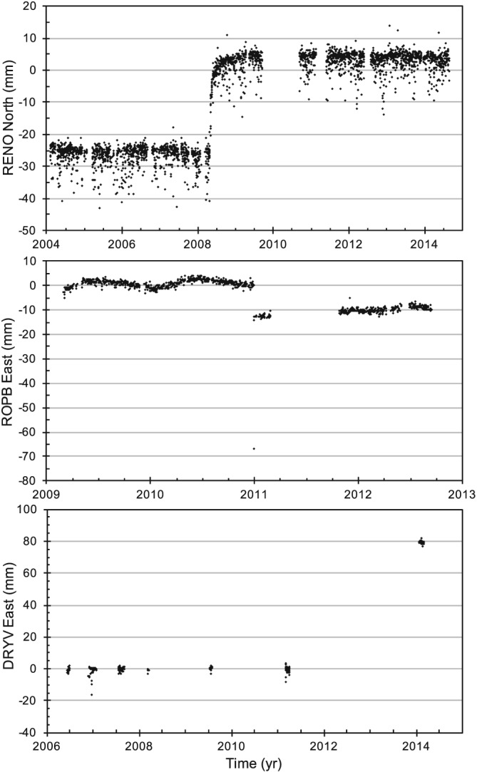
Coordinate time series that have been detrended using the MIDAS velocities for pathological examples detailed in the text: (top) station RENO north component, with an earthquake and skewness; (middle) station ROPB east component, with previously undetected step and outliers; (bottom) station DRYV east component, with displaced monument in the final campaign. Trends agree visually with zero slope lines.

All of these examples and the many others visually inspected so far demonstrate qualitatively that MIDAS is mitigating steps as designed. Moreover, they illustrate how MIDAS can be used as a tool to flag problems with conventional analysis or for flagging time series that deserve further investigation using other tools.

3.2. Accuracy Using Synthetic Data

MIDAS was subject to a blind test using 50 simulated station coordinate time series (each for east, north, and up) that were previously generated for the Detection of Offsets in GPS Experiment (DOGEx) for purposes of testing step detection methods [Gazeaux et al., 2013]. Each of the 150 time series (100 horizontal and 50 up) has a known but undisclosed constant velocity, synthetic steps, gaps, and power law noise. A total of 20 automatic step detection programs from different analysis groups around the world were previously tested blindly by Gazeaux et al. [2013]. Performance can be assessed by comparing the true velocity to the velocity estimated by least squares using all the steps identified by each program (whether true or false).

Since MIDAS does not even attempt to detect steps, we instead blindly tested the accuracy of MIDAS velocities. Only one of the authors had access to the true velocities of the simulated data, while a different author was responsible for producing the MIDAS velocities using the simulated data without ever having access to the true values. Figure 3 shows a histogram of the resulting MIDAS velocity error distribution separately for the horizontal (east and north pooled together) and up components. We first analyze this distribution in terms of central tendency, dispersion, and kurtosis, and then we compare it with distributions from the other estimators (Figures 4 and 5).

Figure 3.

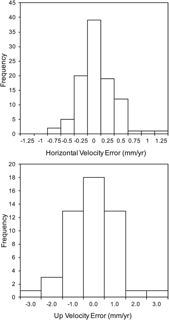
Histograms of MIDAS velocity errors on synthetic time series.

Figure 4.

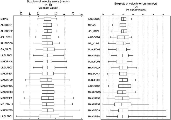
Boxplots summarizing the velocity error distributions using the DOGEx synthetic data for (left) north and east components and (right) up component. Results are from MIDAS and from least squares using steps identified by 16 of the best automatic step detection programs. The box width is the IQR, and the central line is the median. The width between whiskers is the IPR. Boxplots are ranked top to bottom in order of increasing IPR. MIDAS outperforms least squares with step detection.

Figure 5.

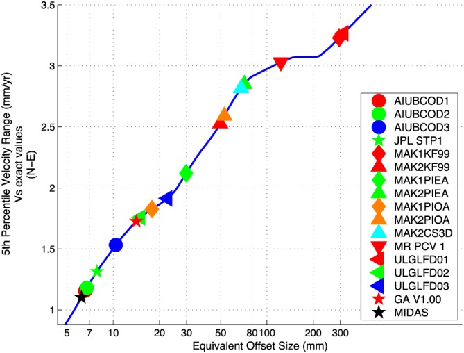
Performance of horizontal velocities estimated by MIDAS compared with least squares using a variety of step detection methods, plotted as IPR (5th percentile range) versus equivalent step detection threshold, as explained by Gazeaux et al. [2013]. Even though MIDAS does not detect steps, it has an equivalent step detection threshold of ~6 mm, lower than actual step detection methods.

First of all, the mean μ of the MIDAS velocity errors is 0.036 ± 0.032 mm/yr horizontal and −0.07 ± 0.15 mm/yr up, which are statistically consistent with zero for normally distributed errors. The dispersion of the velocity error distribution from the 150 synthetic time series was analyzed using three statistics: (1) the RMS velocity error, which is the standard deviation about 0; (2) the “IQR” interquartile range (P ₇₅–P ₂₅); and (3) the “IPR” interpercentile range (P ₉₅–P ₅). The rationale for these statistics is as follows: (1) the RMS includes all solutions, whether good or bad, and gives a measure that can be directly compared with MIDAS uncertainties and with measures of accuracy tested on real data; (2) for a symmetric distribution, the IQR is simply twice the MAD of velocity estimates and is therefore a robust measure of dispersion, quantifying how well the estimator performs most of the time; (3) the IPR is insensitive to the few most extreme values in each tail yet will reflect poor performance should an excessive number of outliers exist. For a normal distribution of standard deviation σ, the IQR and IPR correspond to 1.35σ and 3.29σ, respectively, with a ratio IPR/IQR = 2.44. Increasing the number of outliers increases this ratio.

The results on the measures of dispersion of the MIDAS velocity errors are as follows: (1) the RMS is ±0.33 mm/yr horizontal and ±1.07 mm/yr up, (2) the IQR is 0.41 mm/yr horizontal and 1.20 mm/yr up, and (3) the IPR is 1.10 mm/yr horizontal and 3.54 mm/yr up. The measures of dispersion are ~3 times larger for up than the horizontal, which we assume reflects the DOGEx model for simulating data. This ratio is a common rule‐of‐thumb in GPS geodesy. In comparison, the RMS uncertainty computed by MIDAS is ±0.41 mm/yr horizontal and ±0.91 mm/yr up. Thus, the overall magnitude of the MIDAS uncertainties is therefore reasonably consistent with the dispersion of actual errors, a consequence of our scaling of the standard errors by the factor of 3 to compute the uncertainty in equation (8).

As a further test that MIDAS velocity errors closely follow the normal distribution without excessive frequency of outliers, we follow Folk and Ward [1957] by defining “graphic kurtosis”:

$$K=\frac{1}{2.44}\frac{\mathrm{I}\mathrm{P}\mathrm{R}}{\mathrm{I}\mathrm{Q}\mathrm{R}}$$ (9)

This has a value of 1.0 for the normal distribution. Distributions with heavy tails and sharped peakness relative to the normal distribution have larger kurtosis [DeCarlo, 1997]. The graphic kurtosis for MIDAS velocity errors is 1.11 horizontal and 1.21 up, which are considered close to that of the normal distribution [Folk and Ward, 1957].

The MIDAS velocity errors distribution was then compared to distributions resulting from least squares estimation that include steps that were identified from each of 20 automatic programs from around the world. The sample distributions are summarized using a boxtail plot in Figure 4. Boxes from the worst four programs tested are not shown. Of all methods tested, the velocity error distribution for MIDAS shows the smallest IPR in the horizontal components (100 samples) and the second smallest IPR in the up component (50 samples). MIDAS also has the smallest IQR for the horizontal components.

The DOGEx also quantified and compared the equivalent offset size that could be detected by each step detection method. To some degree, this statistic is sensitive to the distribution of step sizes assumed by DOGEx, but it does give an impression on relative performance. Figure 5 shows that for horizontal components, MIDAS has an equivalent offset size at ~6 mm, which is smaller than from any step detection algorithm. Overall, the DOGEx results indicate that MIDAS performs at least as well as least squares coupled with the best automatic step detectors.

In comparisons with manual screening by five different international experts (not shown), only one method slightly exceeded the performance of MIDAS by a level that is not statistically significant. Thus, MIDAS is an automatic method of velocity estimation that performs as well as the best human experts.

3.3. Accuracy Using Real Data

The no‐net rotation condition of the published North America‐fixed reference frame, NA12, is realized by 30 core stations that have long, manually screened, well‐behaved time series [Blewitt et al., 2013]. These stations lie in the stable interior of the North America tectonic plate far from geophysical processes that deform the crust. We can therefore test the accuracy of velocity estimates under the assumption that these stations have true velocities of zero in the no‐net rotation frame. These stations were not selected on the basis of the magnitude of their horizontal velocity estimates; hence, these estimates provide an absolute test of accuracy (or at least an upper limit). Given that one of the criteria for selecting these stations was the quality of the least squares residuals, such time series are near‐optimal for least squares velocity estimation. The results are shown in Figure 6.

Figure 6.

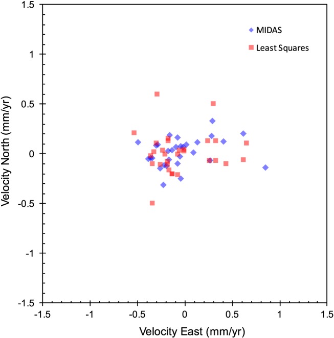
Accuracy of estimated horizontal velocities of stations in the deep interior of the North American plate, where it is assumed that the plate is rigid. Blue diamonds show results of our MIDAS estimator, and red crosses show the published NA12 reference frame velocities estimated using least squares on step‐free data [Blewitt et al., 2013]. MIDAS uncertainties are not shown for clarity; however, they are consistent with the scatter of the data.

We quantify accuracy of the horizontal velocity components by the RMS scatter about zero. The RMS is ±0.26 mm/yr for least squares and ±0.23 mm/yr for MIDAS. Therefore, both methods have similar accuracy for the NA12 core stations. This confirms the expectation that MIDAS competes with least squares when applied to prescreened, well‐behaved data.

In comparison, the RMS uncertainty in horizontal velocity components over all 30 stations as computed by equations (6), (7), (8) is ±0.14 mm/yr. The RMS uncertainty is significantly lower than the observed RMS. If the uncertainties are realistic, then this difference would suggest there exists real intraplate deformation in North America at a level ±0.2 mm/yr, slightly below the level allowed by previous published results [Calais et al., 2006; Blewitt et al., 2013].

We cannot test the up component in a similar way, because the quality of the up velocity was already used as a criterion to select the horizontal time series by Blewitt et al. [2013]. Nevertheless, the RMS velocity difference between MIDAS and least squares is ±0.5 mm/yr, which can be considered a measure of precision rather than accuracy.

Finally, we tested the processing time for a much broader set of real‐world data with mean time series duration of 9 years. The processing time on a single CPU of a laptop computer was 0.08 s per time series (for single coordinates). Considering that the computational complexity is approximately linear in time, this implies ~0.01 s per year of data.

3.4. Performance Using Campaign Data

We do not expect the MIDAS estimator to be as resistant to seasonality and problem in time series when processing GPS campaign data that are sparse in time. Nevertheless, it was previously demonstrated in Figure 2 for campaign station DRYV that MIDAS can mitigate the effect of monument relocation.

Here we test the performance of MIDAS on time series from our ~400 station MAGNET (Mobile Array for NEvada Transtension) semicontinuous network, for which antennas are mechanically constrained to be installed at precisely the same location for every campaign visit [Blewitt et al., 2009]. Some of the MAGNET stations are located sufficiently near to continuously operating stations of the Plate Boundary Observatory, such that, geophysically, we can consider their velocities to be identical. This allows us to conduct engineering tests (such as this one) to assess the quality of MAGNET velocity solutions and their relationship to MIDAS uncertainty for campaign data.

We selected 11 such pairs of stations. The number of campaigns per station ranged from 7 to 17 with a mean of 11.9. For campaign stations, the time series span ranged from 6 to 10 year with a mean of 8.6 year. The mean number of days sampled per year was 61.5 therefore on average 17% of days had data for a campaign station (versus ~100% for a continuous station).

Results of the differences in estimated MIDAS velocities between each station pair are presented in Table 1. The RMS differences are 0.15 mm/yr horizontal and 0.74 mm/yr up. The RMS uncertainty for these differences (pessimistically assuming zero correlation) is 0.26 mm/yr horizontal and 1.16 mm/yr up. Not shown on Table 1, the MAGNET RMS uncertainty is 0.23 mm/yr horizontal and 1.00 mm/yr up. Also not shown, the MAGNET RMS up velocity is 0.74 mm/yr, which can be taken as an upper bound on vertical rate accuracy (as it neglects any real geophysical vertical rates). This demonstrates that the velocity uncertainty is realistic for MAGNET campaigns and that MAGNET campaigns can deliver sub‐mm/yr accuracy and precision, competitive with continuously operating stations.

Table 1.

Differences of MIDAS Velocities for Pairs of Nearby Stations^a

Station 1	Station 2	Velocity 2–Velocity 1 (mm/yr)
Campaign	Continuous	East	North	Up
BLAC	P096	0.21 ± 0.26	−0.15 ± 0.29	−0.67 ± 1.06
CINN	P097	0.11 ± 0.26	0.10 ± 0.26	0.30 ± 1.14
DVAL	P143	−0.24 ± 0.36	−0.08 ± 0.34	−1.36 ± 1.68
GARC	GARL	−0.12 ± 0.19	0.19 ± 0.21	0.50 ± 0.78
JERS	P083	0.32 ± 0.26	−0.05 ± 0.23	−0.55 ± 0.92
KYLE	P078	0.16 ± 0.20	−0.17 ± 0.19	−0.27 ± 0.90
RPAS	P071	−0.14 ± 0.35	−0.01 ± 0.42	0.25 ± 1.91
SKED	P151	−0.10 ± 0.22	−0.23 ± 0.26	−1.26 ± 1.17
UHOG	UPSA	0.05 ± 0.17	−0.14 ± 0.18	−0.72 ± 0.80
VIGU	P002	−0.01 ± 0.19	−0.07 ± 0.23	0.14 ± 0.76
VIRP	P095	0.22 ± 0.27	0.02 ± 0.30	−0.90 ± 1.00
	RMS	0.17 ± 0.25	0.13 ± 0.27	0.74 ± 1.16

^aError bars are the root‐sum‐square of MIDAS uncertainties for each pair.

We conclude that MIDAS performs extremely well with MAGNET‐style campaign data. Finally, we note that processing of campaign stations should obviously be much faster than for continuous stations. The processing time for 369 MAGNET stations (1107 time series) was 16 s on a single CPU.

4. Conclusions

We have developed MIDAS, a new estimator of GPS station velocity, designed to be resistant to seasonal signals, outliers, step discontinuities, and heteroscedasticity. Unlike current methods based on conventional least squares, MIDAS does not attempt to detect step discontinuities. MIDAS is based on the Theil‐Sen median trend estimator with two design features to mitigate steps: (1) slope samples from pairs of data are preferentially selected using data separated by 1 year and (2) the median is iterated once after removing slope outliers that exceed an estimated 2 standard deviations from the median value. Theoretically, the number of arbitrarily large steps that can be tolerated is (T–1)/2, where T is the span of the time series in years, thus, 3 years is the minimum span to be resistant to a single step. Continuous time series spanning 3 years can tolerate 17% of data being outliers. Asymptotically, the very longest time series can tolerate up to 25% of data being outliers.

We have tested MIDAS accuracy using real data and synthetic data. Results from both types of test are consistent with each other. To summarize our findings, (1) MIDAS ranks best in blind tests of velocity accuracy over schemes that couple least squares estimation together with 20 different automatic step detection programs; (2) MIDAS proves to be robust when subject to synthetic data with step discontinuities, producing velocity errors that are realistic and approximately normally distributed; (3) MIDAS velocities for various time series tested have an RMS error of ~0.3 mm/yr horizontal and ~1.0 mm/yr up, consistent with computed uncertainties; and (4) MIDAS performs well on campaign data and effectively rejects data from campaigns that have antenna setup blunders Unlike the ordinary Theil‐Sen estimator, MIDAS computation time scales linearly with the number of data. Using the well‐established quickselect algorithm to find percentile values, computation is ~0.1 s per time series.

We suggest that (1) MIDAS may be implemented to improve current step detectors by providing a robust initial estimate of the trend less biased by undetected steps; then (2) knowing the timing of each step could be used to improve MIDAS by elimination of affected slopes. This integration of MIDAS together with conventional methods is ultimately necessary for applications such as reference frame realization, for which station velocity alone is of limited value. MIDAS should also be useful as an independent check on conventional methods for a variety of applications.

We conclude that MIDAS is suitable for automatic generation of velocity estimates and uncertainties for publication and for automated operational analysis, for example, on our web pages at http://geodesy.unr.edu that include ~40,000 time series, which are updated every week without need for manual screening, step detection, and the associated bookkeeping. MIDAS is well tested and ready to contribute to many research activities. Considering its general nature, MIDAS has the potential for broader application in the geosciences beyond that of GPS velocity estimation, particularly to time series that exhibit seasonality, red noise, and artificial steps caused by equipment configuration changes, such as tide gauge data.

Appendix A. MIDAS Breakdown Point

The sample breakdown point is defined, as the number of data with arbitrary problems that can be tolerated before the estimate becomes arbitrarily large. This is not a probabilistic statistic; rather, it is deterministic assuming the worst possible scenario, however, unlikely it may be. Here we derive the breakdown point analytically for continuous time series (without gaps) applicable to both the interannual Theil‐Sen estimator and the MIDAS estimator. We first consider the case of arbitrarily large outliers and then consider the case of arbitrarily large step discontinuities.

The MIDAS data pair selection algorithm is applied symmetrically in time, firstly, in time order (forward) and secondly, in reverse time order (backward). For the case of continuous data (without gaps), all data pairs are selected twice. Therefore, we only need to consider the application of MIDAS forward in time. Also, we will not be concerned with the insignificant detail as to whether integers are odd or even.

Let there be n coordinate data, of which n ₀ are good and n ₁ are bad at the point of breakdown. These coordinate data are used to compute slopes from m data pairs, of which m ₀ are good and m ₁ are bad:

$$\begin{array}{c}n=n_0+n_1\\ m=m_0+m_1\end{array}$$ (A1)

So that we can express breakdown point more intuitively as a function of time span rather than number of data, let us define the time span in years simply as the dimensionless quantity:

$$T\text{≡}\frac{n}{365}$$ (A2)

Similarly, it is convenient to define the sample breakdown point as the dimensionless quantity:

$$T_1\text{≡}\frac{n_1}{365}$$ (A3)

The fractional breakdown point is defined:

$$b\text{≡}\frac{n_1}{n}=\frac{T_1}{T}$$ (A4)

Given that the median has a breakdown point of 50%, we can write

$$m_1=\frac{m}{2}$$ (A5)

Now let us assume the worst‐case situation, for which all bad coordinate data are paired with two good data to form two bad pairs. Therefore, the breakdown point satisfies

$$n_1=\frac{m_1}{2}=\frac{m}{4}$$ (A6)

Substituting (A6) into (A3) gives the breakdown point as a function of number of pairs:

$$T_1=\frac{1}{4}\frac{m}{365}$$ (A7)

Moving forward through the time series, each data can be paired with another 1 year ahead, except for the last year of data. Therefore, the total number of pairs is

$$m=n-365=365\left(T-1\right)$$ (A8)

Substituting (A8) into (A7) gives the breakdown point in years as a function of time span:

$$T_1=\frac{1}{4}\left(T-1\right)$$ (A9)

Hence, from equation (A4) the fractional breakdown point is

$$b=\frac{1}{4}\left(1-\frac{1}{T}\right)$$ (A10)

This is the asymptotic breakdown point. Note that for large T, the b tends to 25%. We now find the minimum range of T for which it is possible to have the worst‐case situation, equation (6). To match pairs twice, the bad data must all fall within the range from 1 year to T–1 years, which is a range that spans T–2 years. Therefore, all the good data must be at least within the first and last years, spanning 2 years, hence the following inequalities:

$$\begin{array}{l}{n}_0>2\times 365\\ n_1<n-2\times 365\\ T_1<T-2\end{array}$$ (A11)

From equations (A11) and (A9), we therefore have the inequality:

$$\begin{array}{l}\frac{1}{4}\left(T-1\right)<T-2\\ T>\frac{7}{3}\end{array}$$ (A12)

Hence, equations (A9) and (A10) apply to time series longer than 2⅓ years:

$$b=\frac{1}{4}\left(1-\frac{1}{T}\right)\text{if}T>2\raisebox{1ex}{$1$}\!\left/ \!\raisebox{-1ex}{$3$}\right.$$ (A13)

For shorter time series, consider that for spans between 1 and 2 years, no data can be paired twice. Therefore, the worst case is that each bad data point is paired once with a good data point. Thus, the breakdown point is twice that of (A13):

$$\frac{1}{2}\left(1-\frac{1}{T}\right)\text{if}1<T<2$$ (A14)

Note that as the span gets smaller and approaches 1 year, the breakdown point goes to zero, and therefore, MIDAS looses robustness. Between these extremes, the ratio of bad data that are paired once to those that are paired twice can be interpolated, leading to the following expression:

$$b=\frac{1}{4}\left(8-3T\right)\left(1-\frac{1}{T}\right)\text{if}2\le T\le 2\raisebox{1ex}{$1$}\!\left/ \!\raisebox{-1ex}{$3$}\right.$$ (A15)

Now we derive the step breakdown point, M, which we define as the number of arbitrary steps that MIDAS can tolerate. For a given number of steps M, the worst‐case scenario is if steps are at least 1 year apart, because this maximizes the number of bad data pairs spanning the steps:

$$m_1=365M$$ (A16)

From (A5) and (A8), the breakdown point is satisfied by

$$m_1=\frac{365}{2}\left(T-1\right)$$ (A17)

Substituting (A17) into (A16) gives the step breakdown point:

$$M=\frac{T-1}{2}$$ (A18)

which must be rounded down to the nearest integer value to give the maximum number tolerable. Table A1 gives numerical examples of the analytical results derived here.

Table A1.

MIDAS Breakdown Point as a Function of Time Span^a

Total Span T(yr)	Outlier Span	Outlier Fraction	Number of Steps
	T 1(year)	b	M
1 = 1.00	0 = 0.00	0 = 0.00	0
1¼ = 1.25	⅛ = 0.12	1/10 = 0.10	0
1½ = 1.50	¼ = 0.25	1/6 = 0.17	0
1¾ = 1.75	⅜ = 0.37	3/14 = 0.21	0
2 = 2.00	½ = 0.50	1/4 = 0.25	0
2⅓ = 2.33	⅓ = 0.33	1/7 = 0.14	0
3 = 3.00	½ = 0.50	1/6 = 0.17	1
4 = 4.00	¾ = 0.75	3/16 = 0.19	1
5 = 5.00	1 = 1.00	1/5 = 0.20	2
7 = 7.00	1½ = 1.50	3/14 = 0.21	3
9 = 9.00	2 = 2.00	2/9 = 0.22	4
15 = 15.00	3½ = 3.50	7/30 = 0.23	7
21 = 21.00	5 = 5.00	5/21 = 0.24	10

^aFor example, with 5 years of data, MIDAS can tolerate 365 outliers (1 year), which is 20% of the data.

Blewitt, G. , Kreemer C., Hammond W. C., and Gazeaux J. (2016), MIDAS robust trend estimator for accurate GPS station velocities without step detection, J. Geophys. Res. Solid Earth, 121, 2054–2068, doi:10.1002/2015JB012552.

References

- Agnew, D. C. (1992), The time‐domain behavior of power‐law noises, Geophys. Res. Lett., 19(4), 333–336, doi:10.1029/91GL02832. [Google Scholar]
- Akritas, M. G. , Murphy S. A., and LaValley M. P. (1995), The Theil‐Sen estimator with doubly censored data and applications to astronomy, J. Am. Stat. Assoc., 90(429), 170–177. [Google Scholar]
- Blewitt, G. , and Lavallée D. (2002), Effect of annual signals on geodetic velocity, J. Geophys. Res., 107(B7), 2145, doi:10.1029/2001JB000570. [Google Scholar]
- Blewitt, G. , Kreemer C., and Hammond W. C. (2009), Geodetic observation of contemporary deformation in the northern Walker Lane: 1. Semipermanent GPS strategy, Late Cenozoic Structure and Evolution of the Great Basin—Sierra Nevada Transition, Geol. Soc. Am., 447, 1–15, doi:10.1130/2009.2447(01). [Google Scholar]
- Blewitt, G. , Kreemer C., Hammond W. C., and Goldfarb J. M. (2013), Terrestrial reference frame NA12 for crustal deformation studies in North America, J. Geodyn., 72, 11–24, doi:10.1016/j.jog.2013.08.004. [Google Scholar]
- Brody, J. J. (1969), Zero‐crossing statistics of 1/f noise, J. Appl. Phys., 40(2), 567–569. [Google Scholar]
- Calais E., Han J. Y., DeMets C., and Nocquet J. M. (2006), Deformation of the North American plate interior from a decade of continuous GPS measurements, J. Geophys. Res., 111, B06402, doi:10.1029/2005JB004253. [Google Scholar]
- DeCarlo, L. (1997), On the meaning and use of kurtosis, Psychol. Meth., 2(3), 292–307. [Google Scholar]
- Fernandes, R. , and Leblanc S. G. (2005), Parametric (modified least squares) and non‐parametric (Theil‐Sen) linear regressions for predicting biophysical parameters in the presence of measurement errors, Rem. Sens. Environ., 95(3), 303–316. [Google Scholar]
- Folk, R. L. , and Ward W. C. (1957), Brazos River bar: A study in the significance of grain size parameters, J. Sediment. Petrol., 27(1), 3–26. [Google Scholar]
- Gazeaux, J. , et al. (2013), Detecting offsets in GPS time series: First results from the detection of offsets in GPS experiment, J. Geophys. Res. Solid Earth, 118, 1–11, doi:10.1002/jgrb.50152. [Google Scholar]
- Griffiths, J. , and Ray J. R. (2013), Sub‐daily alias and draconitic errors in IGS orbits, GPS Solutions, 17(3), 413–422, doi:10.1007/s10291-012-0289-1. [Google Scholar]
- Helsel D. R., and Hirsch R. M. (2002), Statistical methods in water resources. USGS Publication, 524 pp. [Available at http://pubs.usgs.gov/twri/twri4a3/pdf/twri4a3‐new.pdf.]
- Hirsch, R. M. , Slack J. R., and Smith R. A. (1982), Techniques of trend analysis for monthly water quality data, Water Resour. Res., 18(1), 107–121, doi:10.1029/WR018i001p00107. [Google Scholar]
- Hoare, C. A. R. (1961), Algorithm 65: Find, Commun. ACM, 4(7), 321–322, doi:10.1145/366622.366647. [Google Scholar]
- Kenney, J. F. , and Keeping E. S. (1954), Mathematics of Statistics, Pt. 1, 3rd ed., 348 pp., Van Nostrand, New York. [Google Scholar]
- Kreemer, C. , Blewitt G., and Klein E. C. (2014), A geodetic plate motion and Global Strain Rate Model, Geochem. Geophys. Geosyst., 15, 3849–3889, doi:10.1002/2014GC005407. [Google Scholar]
- Leys, C. , Klein O., Bernard P., and Licata L. (2013), Detecting outliers: Do not use standard deviation around the mean, use absolute deviation around the median, J. Exp. Soc. Psychol., 49(4), 764–766, doi:10.1016/j.jesp.2013.03.013. [Google Scholar]
- Sen, P. K. (1968), Estimates of the regression coefficient based on Kendall's tau, J. Am. Stat. Assoc., 63, 1379–1389. [Google Scholar]
- Stigler, S. M. (1981), Gauss and the invention of least squares, Ann. Stat., 9(3), 465–474. [Google Scholar]
- Theil, H. (1950), A rank‐invariant method of linear and polynomial regression analysis, Indag. Math., 12, 85–91. [Google Scholar]
- Wilcox, R. R. (2005), Introduction to Robust Estimation and Hypothesis Testing, Elsevier Academic Press, Burlington, Mass. [Google Scholar]
- Williams, S. D. P. (2003), Offsets in Global Positioning System time series, J. Geophys. Res., 108(B6), 2310, doi:10.1029/2002JB002156. [Google Scholar]
- Williams, S. D. P. , Bock Y., Fang P., Jamason P., Nikolaidis R. M., Prawirodirdjo L., Miller M., and Johnson D. J. (2004), Error analysis of continuous GPS position time series, J. Geophys. Res., 109, B03412, doi:10.1029/2003JB002741. [Google Scholar]
- Zięba, A. , and Ramsa P. (2011), Standard deviation of the mean of autocorrelated observations estimated with the use of the autocorrelation function estimated from the data, Metrol. Meas. Syst., 18(4), 5329–5542, doi:10.2478/v10178-011-0052-x. [Google Scholar]