

Abstract
Osteoarthritis (OA) is the most common form of joint disease and often characterized by cartilage changes. Accurate quantitative methods are needed to rapidly screen large image databases to assess changes in cartilage morphology. We therefore propose a new automatic atlas-based cartilage segmentation method for future automatic OA studies.
Atlas-based segmentation methods have been demonstrated to be robust and accurate in brain imaging and therefore also hold high promise to allow for reliable and high-quality segmentations of cartilage. Nevertheless, atlas-based methods have not been well explored for cartilage segmentation. A particular challenge is the thinness of cartilage, its relatively small volume in comparison to surrounding tissue and the difficulty to locate cartilage interfaces – for example the interface between femoral and tibial cartilage.
This paper focuses on the segmentation of femoral and tibial cartilage, proposing a multi-atlas segmentation strategy with non-local patch-based label fusion which can robustly identify candidate regions of cartilage. This method is combined with a novel three-label segmentation method which guarantees the spatial separation of femoral and tibial cartilage, and ensures spatial regularity while preserving the thin cartilage shape through anisotropic regularization. Our segmentation energy is convex and therefore guarantees globally optimal solutions.
We perform an extensive validation of the proposed method on 706 images of the Pfizer Longitudinal Study. Our validation includes comparisons of different atlas segmentation strategies, different local classifiers, and different types of regularizers. To compare to other cartilage segmentation approaches we validate based on the 50 images of the SKI10 dataset.
Keywords: Cartilage, Atlas, Segmentation, Three-label, Automatic
1. Introduction
Osteoarthritis (OA) is the most common form of joint disease and a major cause of long-term disability in the United States of America (Woolf and Pfleger, 2003). Cartilage loss is believed to be the dominating factor in OA. As magnetic resonance imaging (MRI) is able to evaluate cartilage volume and thickness and allows reproducible quantification of cartilage morphology (Eckstein et al., 1998; Eckstein et al., 2006) it is increasingly accepted as a primary method to evaluate progression of OA. An accurate cartilage segmentation from magnetic resonance (MR) knee images is crucial to study OA and would be of particular use for future clinical trials to test so far non-existing disease-modifying OA drugs. Already today, large image databases exist for OA studies which are well suited to design and test automatic cartilage segmentation algorithms capable of processing thousands of images. For example, the Pfizer Longitudinal Study (PLS) dataset contains 158 subjects, each with five time points. The Osteoarthritis Initiative (OAI) dataset includes 4796 subjects with multiple time points. Due to the large size of image databases, a fully automatic segmentation and analysis method is essential. In this paper, we therefore propose a new cartilage segmentation method from knee MR images, which requires no user interaction (besides quality control). The method is a step towards automatic analysis of large OA image databases.
Recently, several automatic methods have been proposed for cartilage segmentation. Folkesson et al. (2007) proposed a voxel-based hierarchical classification scheme for cartilage segmentation. Fripp et al. (2010) used active shape models for bone segmentation in order to extract the bone-cartilage interface followed by tissue classification. A graph-based simultaneous segmentation of bone and cartilage was developed by Yin et al. (2010). Vincent et al. (2010) applied multi-start and hierarchical active appearance modeling to segment cartilage. Texture analysis (Dodin et al., 2010) has also been employed in cartilage segmentation. Seim et al. (2010) utilized prior knowledge on the variation of cartilage thickness. Voxel-based classification approaches have been investigated for segmenting multi-contrast MR data in (Koo et al., 2009; Zhang and Lu, 2011).
To allow for localized analysis and the suppression of unlikely voxels in a segmentation, introducing a spatial prior is desirable. This can be achieved through an atlas-based analysis method. In particular, multi-atlas segmentation strategies (Rohlfing et al., 2004) have shown to be robust and reliable image segmentation methods. While such methods have been successfully used in brain imaging, they have so far rarely been used for cartilage segmentation. The work by Glocker et al. (2007), which used a statistical shape atlas from a set of pre-aligned knee images, and the work by Tamez-Peña et al. (2012) using a multi-atlas-based method, are two exceptions. Our work in this paper is most closely related to (Tamez-Peña et al., 2012) as both methods make use of multi-atlas segmentation strategies. However, we significantly extend the prior work by Tamez-Peña et al. (2012). In particular:
We propose a convex three-label segmentation method which allows for anisotropic spatial regularization. This is a generally applicable segmentation method. Applied to the segmentation of femoral and tibial cartilage, it guarantees their spatial separation while ensuring spatially smooth solutions accounting for the cartilage thinness through anisotropic regularization. We incorporate spatial priors via atlas information (see 2) and local segmentation label likelihoods through appearance classification comparing both k nearest neighbors (kNN) classification and classification by a support vector machine (SVM).
We compare different atlas-based segmentation methods: using a single average-shape atlas as well as multiple atlases with various label fusion strategies as segmentation priors.
We perform an extensive validation on over 700 images with varying levels of OA disease progression using data from both the Pfizer Longitudinal Study (PLS) and from SKI10 (Heimann et al., 2010) to compare to existing methods.
These contributions are significant as:
Due to its convexity our segmentation method allows the efficient computation of globally optimal solutions for three segmentation labels. Furthermore, we demonstrate that anisotropic regularization within this segmentation model is less sensitive to parameter settings than isotropic regularization and yields more accurate segmentations.
We show that using non-local patch-based label fusion from multiple atlases to obtain segmentation priors improves segmentation results significantly over using a single atlas or a local label fusion strategy.
Our validation dataset (with more than 700 images) is at least one order of magnitude larger than most prior cartilage segmentation validation studies, hence demonstrating the ability of our proposed segmentation method to automatically achieve accurate cartilage segmentations for large imaging studies. The required robustness of the segmentation method is achieved by using a multi-atlas segmentation strategy. The obtained accuracy can be attributed to the combination of local classification, multi-atlas label fusion, three-label segmentation and anisotropic regularization.
Fig. 1 illustrates the proposed cartilage segmentation method. The method starts with multi-atlas-based bone segmentation to guide the cartilage atlas registration. The cartilage spatial prior is then obtained from either multi-atlas or average-shape-atlas registration. A probabilistic classification is performed to compute local likelihoods. The three-label segmentation makes the final decision from the spatial priors and the local likelihoods jointly, allowing for anisotropic spatial regularization. The method described in this paper is an extension of the preliminary ideas we presented in recent conference papers (Shan et al., 2010; Shan et al., 2012; Shan et al., 2012b). This paper offers more details, additional experiments, and a much larger validation study.
Fig. 1.
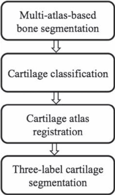
Cartilage segmentation pipeline.
The remainder of this paper is organized as follows: Section 2 clarifies the atlas terminology and briefly reviews the atlas-based segmentation approaches. Section 3 presents the three-label segmentation framework with isotropic and anisotropic regularization. Section 4 describes the multi-atlas-based bone segmentation method. The probabilistic cartilage classification is explained in Section 5. Sections 6 and 7 discuss the average-shape-atlas-based and multi-atlas-based cartilage segmentation, respectively. Experimental results on the PLS dataset are shown in Section 9. We compare the proposed method to other methods in Section 10 by making use of the SKI10 dataset. The paper closes with conclusions and future work.
2. Atlas terminology
An atlas (Aljabar et al., 2009), in the context of atlas-based segmentation, is defined as the pairing of an original structural image and the corresponding segmentation. Atlas-based segmentation methods can be categorized into three groups (Išgum et al., 2009), namely single-atlas-based, average-shape atlas-based and multi-atlas-based methods. The work by Glocker et al. (2007) falls into the second group. The work by Tamez-Peña et al. (2012) belongs to the multi-atlas category.
In the single-atlas-based method, a single labeled image is chosen as the atlas and registered to the query image. The atlas label is propagated following the same transform to generate the segmentation for the query image. The drawbacks of the single-atlas-based segmentation include the possibility that the atlas used is anatomically unrepresentative of the query image and occasional registration failures because the method critically depends on the success of only one registration. To alleviate the problem of being non-representative, average-shape-atlas-based methods have been proposed, where a reference image is selected to build the atlas from a set of labeled images. However, here success still depends on the success of a single registration. Furthermore, the choice of reference image is important for segmentation accuracy and frequently addressed by building an average atlas-image through registration – which in itself is not a trivial task. Alternatively, in multi-atlas-based segmentation, multiple labeled images are registered to the query image independently, hereby avoiding reliance on one registration while allowing to represent anatomical variations. The downside of multi-atlas-based segmentation is high computation cost as multiple registrations are required. In spite of the expensive computation, multi-atlas-based segmentation has been popular and successful in brain imaging. In particular, Rohlfing et al. (2004) demonstrated that multi-atlas-based segmentation is more accurate than the two other atlas-based segmentation methods. We will therefore follow a multi-atlas strategy in what follows.
3. Three-label segmentation method
A binary segmentation consists of only two labels, i.e., foreground and background, and tends to merge touching objects if spatial regularity is enforced. A multi-label segmentation can keep objects separated and is therefore particularly suited to segment touching objects. Since the femoral and tibial cartilage (as well as bones for severe OA patients) may touch each other in the MR images, we make use of a three-label segmentation method to avoid possible mergings. Fig. 2 demonstrates the limitations of a binary versus a three-label segmentation method for a synthetic bone case.
Fig. 2.
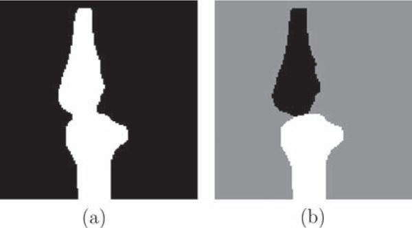
Synthetic example. (a) Binary segmentation result. Femur and tibia are segmented as one object and the boundary in the joint region is not captured well due to regularization effects. (b) Proposed three-label segmentation. The boundaries between bones and background are preserved.
The three-label case is a specialization of our previous multi-label segmentation method (Zach et al., 2009) which allows for a symmetric formulation with respect to the background segmentation class. A multi-label segmentation is a mapping from an image domain Ω to a label space represented by a set of non-negative integers, i.e., ℒ = {0, …, L − 1}. The labeling function Λ: Ω → ℒ, x ↦ Λ(x) maps a pixel x in the image domain Ω to label Λ(x) label space. The goal is to find a labeling function that minimizes an energy functional of the form:
| (1) |
where c(x, Λ(x)) is the cost of assigning label Λ(x) to pixel x and V(·) is a regularizing term. The different labelings can be encoded through a level function u
| (2) |
which maps the Cartesian product of the image domain Ω and the labeling space ℒ to {0, 1}. By definition, we have u(x, 0) = 0 and u(x, L) = 1. Of note, u does not directly encode labels, but instead defines them through its discontinuity set. Fig. 3 illustrates the relation between u and Λ for the three-label case. This setup is in general asymmetric with respect to the labels, since the design of the level function implies a specific label ordering. However, for the three-label case, the background label can be symmetrically positioned between the two object labels (i.e., femoral cartilage and tibial cartilage) hence resulting in a method which treats the two cartilage classes symmetrically.
Fig. 3.
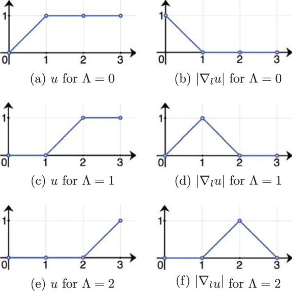
Values of u and |∇lu| for different label assignments in a three-label segmentation (abscissa l). Assuming a discretization with forward differences. |∇lu| determines the label assignment.
Minimizing the segmentation energy functional
| (3) |
with respect to u, results in an essentially binary and monotonically increasing level function u indicating the multi-label image segmentation. Here, ∇xu is the spatial gradient of u, ∇xu = (∂u/∂x, ∂u/∂y, ∂u/∂z)T and ∇lu is the gradient in label direction, ∇lu = ∂u/∂l; g controls the isotropic regularization and c defines the labeling cost. In our implementation, we set g to a non-negative constant. The formulation is convex and therefore a global optimum can be computed. We apply an iterative gradient descent/accent scheme for the optimization. See Appendix A for more details on the numerical solution to (3). The solution u is essentially binary1 and monotonically increasing. The three-label segmentation can then be computed from the discontinuity set of u.
The isotropic regularization in model (3) treats all directions equally, which is not an ideal choice for long and thin objects like the cartilage. To customize the segmentation model (3) for cartilage segmentation, we replace the isotropic regularization term, g, by an anisotropic one
| (4) |
where G is a positive-definite matrix determining the amount of regularization. This avoids over-regularization at the boundaries of the cartilage layers and therefore allows for a more faithful segmentation. Fig. 4 illustrates the problem with isotropic regularization which tends to shrink the segmentation boundary by cutting thin objects short and the benefit from anisotropic regularization. We choose G as
| (5) |
where I is the identity matrix and n is a unit vector indicating the direction of less regularization (the normal direction to the cartilage surface). See Fig. 5 for an illustration of isotropic versus anisotropic regularization. Since the normal direction to the cartilage surface is not known a priori, we approximate it by the normal direction to the bone-cartilage interface which can be determined from the segmentations of femur and tibia (see Section 8). The energy functional (4) is also convex and therefore a global optimum can also be computed. Again, we apply an iterative gradient descent/accent scheme for the optimization. See Appendix A for more details on the numerical solution to (4). The solution u is also essentially binary and monotonically increasing.
Fig. 4.
Synthetic example: (a) original image to be segmented; (b) and (c) three-label segmentation results with isotropic and anisotropic regularization respectively. Anisotropic regularization avoids over-regularization at the tips of the synthetic shape.
Fig. 5.
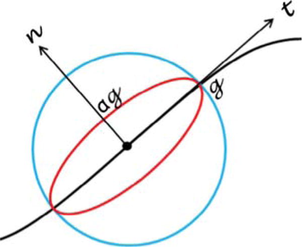
Difference between isotropic and anisotropic regularization. The black curve is an edge in an image. The regularization is illustrated at a pixel (the dot). The blue circle indicates the isotropic case where regularization is enforced equally in every direction. The red ellipse shows the anisotropic situation where less regularization is applied in the normal direction and more in the tangent direction. (For interpretation of the references to color in this figure legend, the reader is referred to the web version of this article.)
Section 4 describes how to use the model (3) for bone segmentation using a multi-atlas-based approach to obtain spatial priors. Details on using model (4) for cartilage segmentation are discussed in Sections 5–7.
4. Multi-atlas-based bone segmentation
The labeling cost c in (3) for each label l in {FB, BG, TB} (“FB”, “BG” and “TB” denote the femoral bone, the background and the tibial bone respectively) are defined by log-likelihoods for each label given image I at a voxel location x:
| (6) |
Note that the background label “BG” is placed in the label order between the femur label “FB” and the tibia label “TB” in order to achieve a symmetric formulation.
The likelihood terms p(I(x)|FB) and p(I(x)|TB) are computed from image intensities. Since bones appear dark in T1 weighted MR images, we assume a simple model (7) to estimate bone likelihoods,
| (7) |
where β is set to 0.02 in our implementation assuming I(x) ∈ [0, 100].
To compute the prior terms p(FB) and p(TB) in (6), we employ a multi-atlas registration approach followed by label fusion. Suppose we have N atlases Ai and their bone segmentations and (i = 1, 2, …, N). Registration from an atlas Ai to a query image I is an affine registration followed by a B-Spline registration . Averaging all N propagated atlas labels yields a spatial prior of femur and tibia for the query image:
| (8) |
Now that we have computed the spatial priors and the local likelihoods, we integrate them into (6) and solve (3) to obtain the three-label bone segmentation. The bone segmentation will help locate the cartilage in atlas-based cartilage segmentation.
5. Probabilistic classification
We use the three-label segmentation with anisotropic regularization for cartilage segmentation to account for thin cartilage layers. The labeling cost c for each label l in {FC, BG, TC} (“FC”, “BG” and “TC” denote the femoral cartilage, the background and the tibial cartilage respectively) are defined by log-likelihoods for each label:
| (9) |
where f(x) denotes a feature vector at a voxel location x. Again the background label “BG” is placed between the femoral cartilage label “FC” and the tibial cartilage label “TC” in order to achieve a symmetric formulation.
We compute the spatial prior p(l) in two different ways: using an average-shape-atlas registration and a multi-atlas registration (see Sections 6 and 7). We compare the performance of both approaches in Section 9. The local likelihood term p(f(x)|l) is obtained from a probabilistic classification based on local image appearance. We investigate classification based on a probabilistic k nearest neighbors (kNN) (Duda et al., 2001) as well as by a support vector machine (SVM) [Cortes and Vapnik, 1995]. For classification we use a reduced set of features compared to (Folkesson et al., 2007): intensities on three scales, first-order derivatives in three directions on three scales and second-order derivatives in the axial direction on three scales. The three different scales are obtained by convolving with Gaussian kernels of σ = 0.3 mm, 0.6 mm and 1.0 mm. All features are normalized to be centered at 0 and have unit standard deviation.
An important difference from (Folkesson et al., 2007; Koo et al., 2009) is the probabilistic nature of our classification which allows for an easy incorporation of the classification result into our Bayesian framework. Further, the final segmentations are generated by a segmentation method with anisotropic regularization, whereas no regularization was used in (Folkesson et al., 2007) nor (Koo et al., 2009). We demonstrate in Section 9 that spatial regularization helps improve the segmentation accuracy and anisotropic regularization yields better accuracy than isotropic regularization.
5.1. Classification using kNN
We estimate the data likelihoods for femoral and tibial cartilage, p(f(x)|l), of (9) by probabilistic kNN classification (Duda et al., 2001). We use a one-versus-other classification strategy and the expert segmentations of femoral and tibial cartilage to build the kNN classifier. Specifically, let “FC” denote the femoral cartilage class, “TC” the tibial cartilage and “BG” the background class. The training samples of class FC are the voxels labeled as femoral cartilage. Similarly, the training samples of class TC are the voxels labeled as tibial cartilage. The training samples of class BG are the voxels surrounding the femoral and tibial cartilage within a specified distance. The outputs of the probabilistic kNN classifier given a query voxel x with its feature vector f(x) are:
| (10) |
Here nFC, nTC, nBG denote the number of votes for the femoral cartilage, tibial cartilage, and background class respectively; k is the number of nearest neighbors of concern. Since kNN is sensitive to the number of training samples, we scale the outputs according to the training class sizes to balance the three classes.
5.2. Classification using an SVM
An alternative approach to compute the local likelihoods is to use a support vector machine (SVM) (Cortes and Vapnik, 1995), which constructs a hyperplane maximally separating classes given a labeled training set. Koo et al. (2009) proposed to use two-class SVM to segment cartilage automatically from multi-contrast MR images. We apply LIBSVM (Chang and Lin, 2011) to perform probabilistic three-class SVM classification with the features described above. The results are local likelihoods for the background, the femoral and the tibial cartilage, i.e., p(f(x)|BG), p(f(x)|FC) and p(f(x)|TC). We compare the SVM and the kNN probabilistic classification methods in Section 9.
6. Average-shape-atlas-based cartilage segmentation
This section discusses how to build a probabilistic bone and cartilage atlas by averaging registered expert segmentations and computing the cartilage spatial priors by registration of the atlas. The atlas within this section captures the spatial relationships between the bone and the cartilage.
Suppose we have N images with expert segmentations. We pick the segmentation of one image as the reference to bring all the segmentations to the same position. Specially, we register the femur segmentation and the tibial segmentation to the reference femur and tibia segmentations with affine transforms and respectively. The femoral and tibial cartilage segmentations and are propagated accordingly. The average bone and cartilage atlas Aavg (including and ) is computed by
| (11) |
Given a query image I, we have computed the bone segmentation SFB and STB from Section 4. The atlas femur AFB and tibia AFB are registered to the segmentation of femur SFB and tibia STB with affine transforms TFB and TTB. The spatial prior for each cartilage is then computed by propagating each cartilage atlas with the corresponding transform,
| (12) |
These spatial priors and the local likelihoods from Section 5 are integrated into (9) and the cartilage segmentation is obtained by optimizing the three-label segmentation energy with anisotropic regularization (4).
7. Multi-atlas-based cartilage segmentation
This section presents an alternative approach to computing the spatial prior for cartilage. We make use of multi-atlas registration, rather than average-shape-atlas registration as described in Section 6. Each atlas is an individual expert bone and cartilage segmentation in this section. Three popular label fusion methods are discussed in this section, i.e., majority voting, locally-weighted and non-local patch-based fusion.
We have N atlases Ai including their femur segmentations , tibia segmentations , femoral cartilage segmentations and tibial cartilage segmentations . For a query image I, we have the bone segmentation SFB and STB from Section 4.
The atlas bone segmentations and are registered to the bone segmentations SFB and STB of the query image separately by affine transforms and .
We can simply take the average of the registered cartilage atlas segmentations to compute the spatial priors, which is majority voting (Rohlfing et al., 2004) label fusion:
| (13) |
We can also apply a locally-weighted label fusion strategy (Išgum et al., 2009), which was shown to yield a better segmentation accuracy than a majority voting strategy. In this case, we choose to favor the atlases which locally agree better with the cartilage likelihoods p(f(x)|FC) and p(f(x)|TC) from the probabilistic classification in Section 5. The spatially varying weighting functions for the femoral cartilage and for the tibial cartilage are calculated as
| (14) |
followed by a small amount of diffusion smoothing. We choose α = 0.2 and ε = 0.001 in our implementation. The spatial prior for each cartilage is then the weighted average of the propagated atlas cartilage segmentations
| (15) |
Recently, non-local patch-based label fusion techniques have been proposed (Coupé et al., 2011; Rousseau et al., 2011). Instead of deciding the label from the same voxel location in each propagated atlas, these methods obtain a label using the surrounding patches in a predefined neighborhood across the training atlases. Weights are assigned to these patches according to the distances between the target patch and the selected patches. This allows local robustness to registrations error.
Let pFC(x and pTC(x), respectively, denote the spatial prior of femoral cartilage (i.e., p(FC)) and tibial cartilage, (i.e., p(TC)) at voxel x. We calculate the probabilities by weighted averages of the propagated labels in a pre-specified search neighborhood across N warped atlases. The weights are determined by local patch similarities. For simplicity, let and . Here, i is the atlas index, running from 1 to refers to the femoral cartilage segmentation of the i-th atlas, and Ii is the i-th atlas appearance. For the femoral cartilage, we have
| (16) |
| (17) |
where x′ is a voxel in the patch centered at x (similarly y′ a voxel in the patch centered at y) and hFC(x) is defined by
| (18) |
Substitute “FB” with “TB” and “FC” with “TC” in superscripts of the equations above for the calculation of pTC(x).
The three label fusion strategies, namely majority voting, locally-weighted and non-local patch-based fusion, are compared in Section 9. The non-local patch-based method is shown to result in the best average segmentation accuracy.
These spatial priors and the local likelihoods from Section 5 are integrated into (9) and the cartilage segmentation is obtained by optimizing the three-label segmentation energy with anisotropic regularization (4).
8. Overall segmentation pipeline
The automatic cartilage segmentation requires expert segmentations of femur, tibia, femoral and tibial cartilage on a set of training images. Given a query knee image, we first correct the MRI bias field (Sled et al., 1998), scale image intensities to a common range, and then perform edge-preserving smoothing using curvature flow (Sethian, 1999).
In the multi-atlas-based bone segmentation, the atlases are registered to the query images with an affine transform followed by a B-spline transform based on mutual information. We compute the average of the propagated atlas bone segmentations as the bone spatial priors. The bone likelihoods are then calculated from the image intensities using (7). The priors and the likelihoods are combined in (6) and then integrated in the three-label segmentation (3), the global optimal solution of which produces the bone segmentation.
Once we have the bone segmentation, we perform the probabilistic classification (kNN or SVM) of knee cartilage in the joint region. The spatial priors for the cartilage can be obtained through registration of an average bone and cartilage atlas, which requires only one registration, or through a multi-atlas registration of cartilage, which needs a number of registrations. If a multi-atlas-based method is chosen, propagated atlas labels are fused (using majority voting, locally-weighted or non-local patch-based label fusion) to obtain the spatial priors. The normal direction n in (5) is computed by taking the gradient of the diffusion smoothed three-label bone segmentation result in-between the joint area. Finally, the local likelihoods and the spatial priors are integrated into the three-label segmentation to generate the cartilage segmentation.
9. Experimental results
9.1. Data description
Our main dataset is a subset of the PLS dataset, containing 706 T1-weighted (3D SPGR) images for 155 subjects, imaged at baseline, 3, 6, 12, and 24 months at a resolution of 1.00 × 0.31 × 0.31 mm3. Some subjects have missing scans. The Kellgren–Lawrence grades (KLG) (Kellgren and Lawrence, 1957) were determined for all subjects from the baseline scans, classifying 82 as normal control subjects (KLG0), 40 as KLG2 and 33 as KLG3.
Expert cartilage segmentations (drawn by a domain expert, Dr. Felix Eckstein) are available for all images. The femoral cartilage segmentation is drawn only on the weight-bearing part while the tibial cartilage segmentation covers the entire region. Therefore, we expect partial femoral cartilage and full tibial cartilage segmentation results.
9.2. Bone validation
Bone segmentation is validated on 18 images because expert segmentations for bones are only available for the baseline images of 18 subjects. We validate our multi-atlas-based bone segmentation method in a leave-one-out manner. Each test image is segmented using the other 17 images as atlases. The segmentation accuracy is evaluated with respect to the expert segmentations using the Dice similarity coefficient (DSC) (Dice, 1945) defined as
| (19) |
where S and R represent two segmentations. Table 1 and Fig. 6 show the validation results of the bone segmentation with and without regularization (corresponding to g > 0 and g = 0 in model (3) respectively). No significant improvement is observed by introducing spatial regularization to the bone segmentation, because the multi-atlas-based spatial prior nicely locates the bones. We can see from Fig. 7 that the multi-atlas-based prior captures the bone very well and our segmentation result is very close to the expert segmentation especially in the joint region. We use the bone segmentation with spatial regularization g = 0.5 to compute the cartilage segmentations for the remaining experiments in this section.
Table 1.
Statistics (mean and standard deviation (STD)) of DSC of bone segmentation on 18 test images with and without spatial regularization.
| g = 0 | g = 0.5 | g = 1.0 | ||
|---|---|---|---|---|
| Femur | Mean | 0.969 | 0.970 | 0.969 |
| STD | 0.011 | 0.011 | 0.011 | |
| Tibia | Mean | 0.966 | 0.967 | 0.966 |
| STD | 0.013 | 0.012 | 0.012 |
Fig. 6.
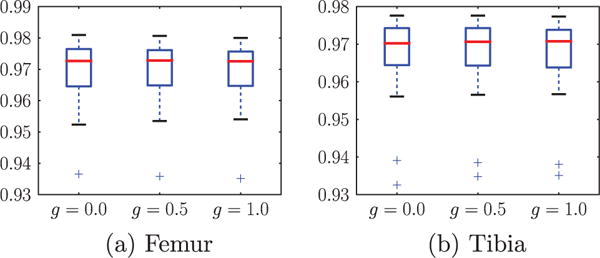
Box plots of DSC for femur and tibia with different amount of regularization on 18 test images. The center red line is the median and the edges of the box are the 25th and 75th percentiles, the whiskers extend to the most extreme data points not considered outliers, and outliers are plotted individually.
Fig. 7.
Bone segmentation of one example slice in coronal view.
9.3. Cartilage validation
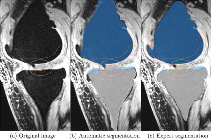
Fig. 8 illustrates the beneficial behavior of our three-label segmentation method compared to a binary segmentation which treats femoral and tibial cartilage as one object. While the three-label method is able to keep femoral and tibial cartilage separated due to the joint estimation of the segmentation, the binary segmentation approach cannot guarantee this separation.
Fig. 8.
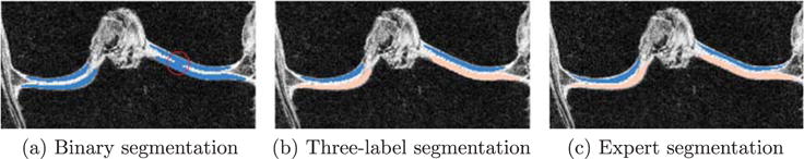
Example comparing binary and three-label segmentation methods. (a) Is the binary segmentation result. (b) Is the three-label segmentation result in which femoral and tibial cartilage have distinct labels. (c) Is the expert segmentation. In (a), as the red circle indicates, the lateral (right) femoral cartilage and tibial cartilage are segmented as one object and the joint boundary is not well captured. The three-label segmentation (b) keeps the femoral and tibial cartilage separate and is therefore superior to binary segmentation.
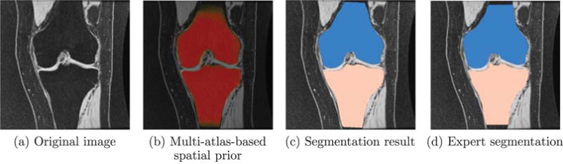
We build an average shape atlas of bone and cartilage from the expert bone and cartilage segmentations of the 18 images. Fig. 9 shows an example slice of the average probabilistic bone and cartilage atlas and the 3-dimensional rendering. The cartilage is well located on top of the bone.
Fig. 9.
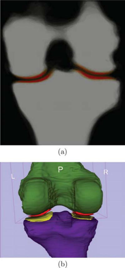
Atlas built from 18 images. (a) is a slice of the probabilistic atlas of femoral and tibial bone and cartilage (red) overlaid on the bone in coronal view. Saturated red denotes high probability. (b) is a 3-dimensional rendering of the thresholded atlas of femur (green), tibia (purple), femoral (red) and tibial cartilage (yellow). (For interpretation of the references to color in this figure legend, the reader is referred to the web version of this article.)
In the average-shape-atlas-based cartilage segmentation, we use the atlas built from 18 images (each from a different subject) to segment cartilage of the remaining 137 subjects. Within the 18 subjects, we test in a leave-one-out manner where each subject is segmented using the atlas built from the other 17 subjects. The same strategy is applied in the multi-atlas-based cartilage segmentation. We use all 18 images as atlases to segment cartilage of the other 137 subjects. The 18 subjects are tested in a leave-one-out fashion. Each subject is segmented using the other 17 images as atlases. The training images for kNN and SVM are chosen in the same way.
In the non-local patch-based label fusion, we upsample the images to approximately isotropic resolution and search for similar 5 × 5 × 5 patches within a 9 × 9 × 9 neighborhood.
Fig. 10 provides an illustration of cartilage segmentation result. Figs. 11 and 12 compare the two local classification methods, i.e., kNN versus SVM, for the femoral and the tibial cartilage, under different atlas choices with varying amount of isotropic spatial regularizations. Note that the femoral cartilage is only segmented in the weight-bearing region and hence the DSC for the femoral cartilage is more sensitive to mis-segmentations than the tibial cartilage. For the femoral cartilage, kNN and SVM generate similar mean DSC. The SVM improves the mean DSC by a considerable amount over the kNN for the tibial cartilage. A possible reason for the similar performance for the femoral cartilage might be that the main disagreement between the automatic and the expert segmentation is along the anterior-posterior direction delineating the weight-bearing region, which may overwhelm any improvement obtained by SVM over kNN. SVM performs better than kNN for tibial cartilage which is segmented in its entirety.
Fig. 10.
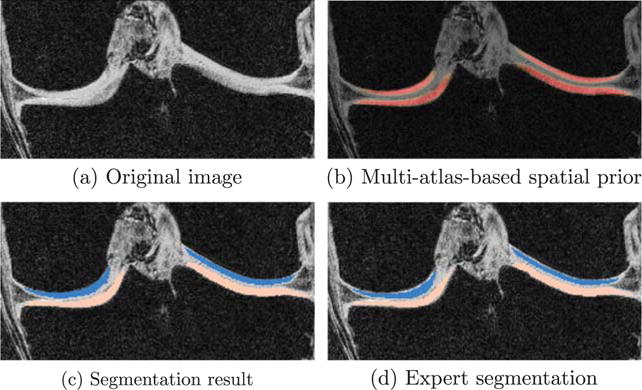
Cartilage segmentation of one example slice in coronal view. Only joint region is shown.
Fig. 11.
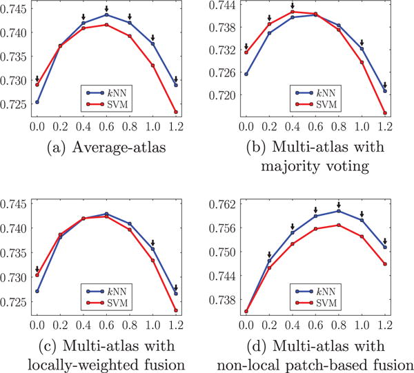
Comparison of kNN and SVM based on the mean DSC (ordinate) with varying amount of isotropic regularization (abscissa g) under different atlas choices for the femoral cartilage. The black downarrows (⇓) indicate statistically significant differences between the two methods at corresponding spatial regularization settings via paired t-tests at a significance level of 0.05.
Fig. 12.
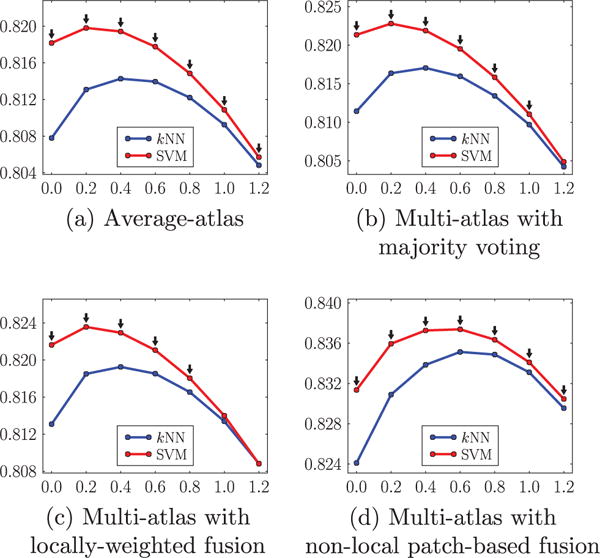
Comparison of kNN and SVM based on the mean DSC (ordinate) with varying amount of isotropic regularization (abscissa g) under different atlas choices for the tibial cartilage. The black downarrows (⇓) indicate statistically significant superiority of SVM to kNN at corresponding spatial regularization settings via paired t-tests at a significance level of 0.05.
Fig. 13 compares the different atlas choices, including the average-shape atlas, multiple atlases with majority voting, locally-weighted and non-local patch-based label fusion, under the different parameter settings of isotropic regularization. The former three yield very similar mean DSC. Non-local patch-based label fusion outperforms the other three considerably. Fig. 14 compare the four atlas choices under the different parameter settings of anisotropic regularization. Again, non-local patch-based label fusion outperforms the other three considerably.
Fig. 13.
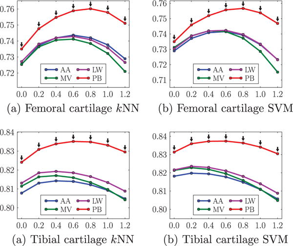
Comparisons of mean DSC (ordinate) from different atlas choices for different amount of isotropic regularization (abscissa g). AA average-shape-atlas. MV multi-atlas with majority voting. LW multi-atlas with locally-weighted fusion. PB multi-atlas with non-local patch-based fusion. The black downarrows (⇓) indicate statistically significant superiority of PB to the other three methods at corresponding spatial regularization settings via paired t-tests at a significance level of 0.05.
Fig. 14.
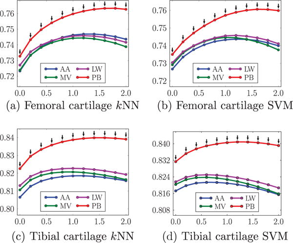
Comparisons of mean DSC (ordinate) from different atlas choices for different amount of anisotropic regularization (abscissa g). The parameter α controlling the anisotropy is set to be 0.2. AA average-shape-atlas. MV multi-atlas with majority voting. LW multi-atlas with locally-weighted fusion. PB multi-atlas with non-local patch-based fusion. The black downarrows (⇓) indicate statistically significant superiority of PB to the other three methods at corresponding spatial regularization settings via paired t-tests at a significance level of 0.05.
Fig. 15 shows the advantage of anisotropic regularization. The isotropic regularization has a tendency to cut long and thin objects short as shown in Fig. 15(a) at the medial femoral cartilage. Anisotropic regularization, on the other hand, avoids this problem (see Fig. 15(b)) resulting in a better segmentation of the medial femoral cartilage. Besides avoiding unrealistic segmentation results, anisotropic regularization is also less sensitive to parameter settings than isotropic regularization. This is illustrated in Fig. 16(a) and (b). Note that the anisotropic regularizer is parametrized in such a way that its regularization is reduced in the normal direction, but equal to the isotropic regularization in the plane orthogonal to the normal and the results are therefore comparable (see Fig. 5). The faster drop-off in the isotropic case indicates a stronger dependency on the parameter settings for isotropic regularization.
Fig. 15.
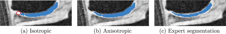
Improvement by anisotropic regularization. (a) Uses isotropic regularization and misses circled region. (b) Uses anisotropic regularization and captures the missing region in (a). (c) Is the expert segmentation.
Fig. 16.
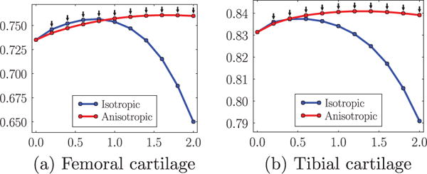
Change of mean DSC for femoral and tibial cartilage with isotropic and anisotropic regularization over the amount of regularization g (abscissa). The parameter a is set to be 0.2 for all anisotropic tests. All tests use SVM and non-local patch-based label fusion. The black downarrows (⇓) indicate statistically significant differences between the two methods at corresponding spatial regularization settings via paired t-tests at a significance level of 0.05.
For anisotropic regularization, to select the “optimal” parameter g for the PLS dataset, we tried different values of g ∈ [0, 2.0] and found that g = 1.4 yields the best average DSC (0.764 and 0.840 for femoral and tibial cartilage respectively) for the 18 training subjects. We apply this “optimal” parameter setting to the test data (the remaining 137 subjects). This setting yields an average DSC of 0.760 for femoral cartilage and 0.841 for tibial cartilage. We use the same parameter setting for a completely independent data set, SKI10 (Heimann et al., 2010), and obtain an average DSC of 0.856 and 0.859 for femoral and tibial cartilage respectively. Even though the “optimal” g could be different for different datasets, the choice of g = 1.4 appeared to be a good candidate for cartilage segmentation. Table 2 summarizes the statistics of segmentation accuracy from 706 images using the best strategy combination.
Table 2.
Statistics summary (mean, median and standard deviation) of DSC under the best strategy combination: SVM and non-local patch-based label fusion with an anisotropic regularization with g = 1.4 and α = 0.2 from the PLS dataset.
| Mean | Median | STD | |
|---|---|---|---|
| Femoral cartilage | 0.760 | 0.768 | 0.048 |
| Tibial cartilage | 0.841 | 0.847 | 0.037 |
As anisotropic regularization is less sensitive to parameter settings, the choice of g does not have a strong impact on segmentation results. Parameter α is set to be 0.2 in our experiments but other values (α ∈ [0, 1]) can also be used. The influence of α will be studied in the future.
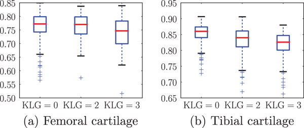
To further illustrate segmentation behavior, we show the box plots of the DSC for different progression levels (i.e., KLGs) for femoral and tibial cartilage in Fig. 17. As expected, we observe a slight deterioration in segmentation accuracy for larger KL grades as it is more challenging to segment pathological knee cartilage.
Fig. 17.
Boxplots of DSC’s for different KLG’s. We choose the best strategy combination, SVM and non-local patch-based label fusion with an anisotropic regularization with g = 1.4 and α = 0.2.
Fig. 18 shows scatter plots of segmentation volumes of the proposed method versus the expert segmentation. The correlation between the volume measured from the expert segmentation and the automatic algorithm achieves a Pearson’s correlation coefficient of 0.77 for all subjects (KLG0: 0.85, KLG2: 0.68, KLG3: 0.74) for the femoral cartilage. For the tibial cartilage, the Pearson’s correlation coefficient is 0.87 for all subjects (KLG0: 0.89, KLG2: 0.80, KLG3: 0.89).
Fig. 18.
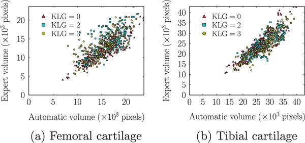
Scatter plots of segmentation volumes (number of pixels). We choose the best strategy combination, SVM and non-local patch-based label fusion with an anisotropic regularization with g = 1.4 and α = 0.2.
The local cartilage thickness is computed from the cartilage segmentation using a Laplace-equation approach (Yezzi and Prince, 2003). We compute the correlation coefficient of local thickness maps from the expert and the proposed segmentations for each image. Fig. 19 shows box plots of Pearson’s correlation coefficients for different KLG’s. Thicknesses of the automatic and the expert segmentations are strongly correlated. Note that correlations for femoral cartilage with respect to volume and thickness are generally lower than for the tibial cartilage due to the fact that only the weight-bearing region of the femoral cartilage is being segmented.
Fig. 19.
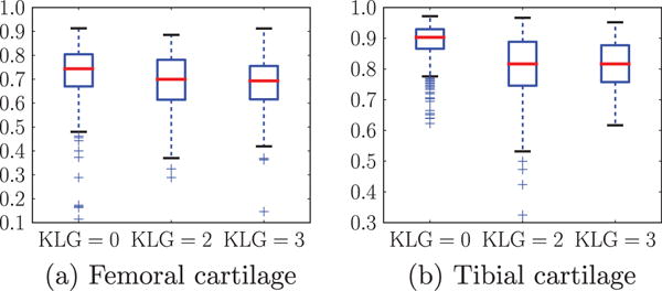
Boxplots of Pearson’s correlation coefficients of local cartilage thickness for different KLG’s. We choose the best strategy combination, SVM and non-local patch-based label fusion with an anisotropic regularization with g = 1.4 and α = 0.2.
9.4. Running time
The overall running time for the segmentation of an MR image is hours. Each atlas registration takes 10–30 min. If registrations are done sequentially, this step takes up to 9 h (as there are 18 atlases). The patch-based label fusion step is completed in 10 min. The local tissue classification takes about 20 min. The computation time for the three-label segmentation varies from minutes to hours. Using anisotropic regularization is slower than isotropic. The running time also depends on the amount of regularization. Large regularization requires more iterations to converge. The segmentation step can be sped up drastically by a GPU implementation, which will be part of the future work.
10. Comparison to other methods
We quantitatively compare methods based on the SKI10 dataset and qualitatively discuss methods which have so far not been tested on SKI10.
10.1. Comparisons based on the SKI10 dataset
To compare to other algorithms we use the data from the cartilage segmentation challenge SKI10 (Heimann et al., 2010). We randomly pick 15 images from the provided 60 training images as atlases to limit computational cost (in principle all 60 images could be used as atlases). SKI10 uses a combined score based on volume difference and volume overlap error for cartilage and bone to score different methods. At time of writing, SKI10 included results for 16 different methods. We restrict ourselves to comparisons between the top 8 methods. The proposed method ranks 5/16 overall. However, as we will discuss below our proposed method performs as well as the top method on volume overlap error for cartilage segmentation (or equivalently Dice coefficient) which as we argue is the most important of the performance measures. For simplicity we denote the methods as Rank 1 to Rank 8 to simplify readability. Tables 3 and 4 contains references and names of the methods as available.
Table 3.
Results of statistical tests (paired t tests for score, VOE and DSC, Wilcoxon signed-rank tests for VD) between different methods. Our method is compared to the other top ranking methods in terms of different measures. Symbol “+” denotes statistically significant superiority of our method; “−” denotes inferiority; “NS” denotes a statistically insignificant difference (p > 0.05). Each table entry consists of two symbols, before and after the correction for multiple comparisons. Rank 7 was also submitted by the authors but using a slightly different combination, i.e., probabilistic kNN and locally-weighted label fusion.
| Rank | Team | Femoral cartilage
|
Tibial cartilage
|
||||||
|---|---|---|---|---|---|---|---|---|---|
| Score | VD | VOE | DSC | Score | VD | VOE | DSC | ||
| 1 | Imorphics Vincent et al. (2010) | NS/NS | +/+ | NS/NS | NS/NS | NS/NS | −/− | NS/NS | NS/NS |
| 2 | ZIB Seim et al. (2010) | NS/NS | +/NS | +/NS | +/NS | NS/NS | −/− | NS/NS | NS/NS |
| 3 | UPMC_IBML | NS/NS | +/+ | +/NS | +/NS | NS/NS | −/− | +/+ | +/+ |
| 4 | SNU_SPL | NS/NS | NS/NS | +/+ | +/+ | NS/NS | NS/NS | +/+ | +/+ |
| 6 | UIiibiKnee Yin et al. (2010) | NS/NS | −/− | +/+ | +/+ | NS/NS | −/− | +/+ | +/+ |
| 7 | shan_unc | NS/NS | +/+ | +/+ | +/+ | NS/NS | −/− | +/+ | +/+ |
| 8 | BioMedIA Wang et al. (2013) | NS/NS | +/+ | +/+ | +/+ | NS/NS | −/− | +/+ | +/+ |
Table 4.
Statistics summary (mean, median and standard deviation) of DSC from the top ranking methods. Rank 7 was also submitted by the authors but using a slightly different combination, i.e., probabilistic kNN and locally-weighted label fusion.
| Rank | Team | Femoral cartilage
|
Tibial cartilage
|
||||
|---|---|---|---|---|---|---|---|
| Mean | Median | STD | Mean | Median | STD | ||
| 1 | Imorphics Vincent et al. (2010) | 0.861 | 0.869 | 0.065 | 0.865 | 0.888 | 0.054 |
| 2 | ZIB Seim et al. (2010) | 0.845 | 0.856 | 0.058 | 0.850 | 0.858 | 0.049 |
| 3 | UPMC_IBML | 0.836 | 0.838 | 0.028 | 0.805 | 0.807 | 0.057 |
| 4 | SNU_SPL | 0.821 | 0.838 | 0.059 | 0.824 | 0.841 | 0.058 |
| 5 | shan_unc (proposed) | 0.856 | 0.862 | 0.057 | 0.859 | 0.861 | 0.047 |
| 6 | UIiibiKnee Yin et al. (2010) | 0.824 | 0.842 | 0.067 | 0.825 | 0.834 | 0.056 |
| 7 | shan_unc | 0.828 | 0.836 | 0.060 | 0.820 | 0.826 | 0.051 |
| 8 | BioMedIA Wang et al. (2013) | 0.840 | 0.854 | 0.062 | 0.836 | 0.841 | 0.048 |
Note that the SKI10 dataset is very challenging as its data was collected from pre-surgery cases, which exhibit severe cartilage damage. It should therefore be regarded as complementing the OAI and the PLS data for validation which cover a much broader range of cartilage degeneration and damage. In particular, the performance of an algorithm on the PLS or OAI data may be more informative for future clinical drug trials aimed at showing small changes in cartilage in relation to therapy.
Fig. 20 shows different measures for femoral and tibial cartilage from the top 8 methods The volumetric difference and volumetric overlap error (VOE) are defined as follows, given a segmentation S and a reference segmentation R.
| (20) |
| (21) |
Fig. 20.
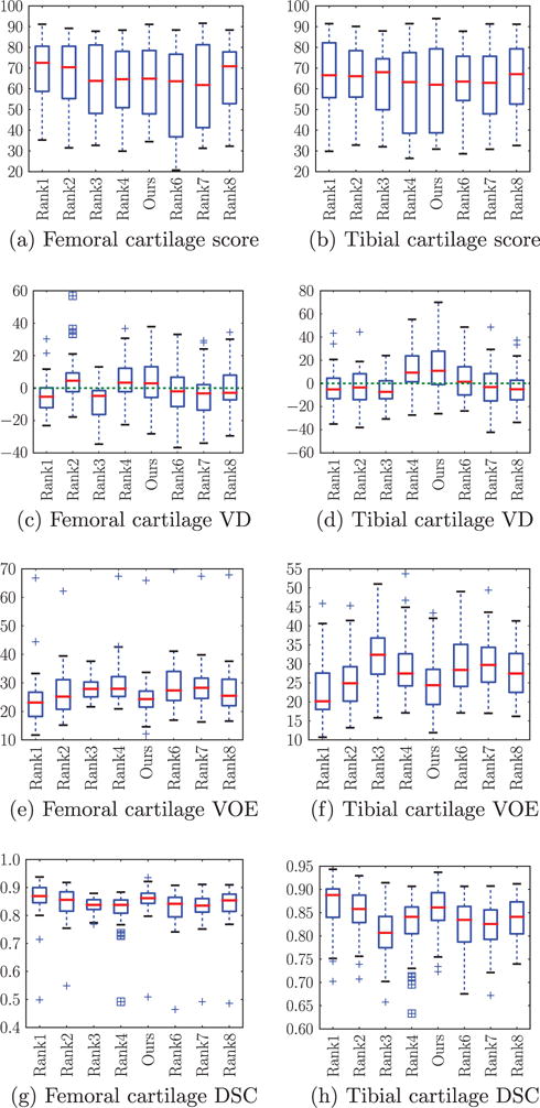
Box plots of segmentation measures for femoral and tibial cartilage from top 8 ranking methods on SKI10 website. The center red line is the median and the edges of the box are the 25th and 75th percentiles, the whiskers extend to the most extreme data points not considered outliers, and outliers are plotted individually. (For interpretation of the references to color in this figure legend, the reader is referred to the web version of this article.)
The challenge defined a scoring system based on inter-observer variations of VD and VOE. On a range from 0 to 100 (meaning a perfect segmentation), a second rater’s outcome corresponds to 75, a result with error twice as high gets 50 and so on. The Dice coefficient can be computed from the VOE as follows
| (22) |
Our method achieves excellent performance on VOE and DSC. The VD is best at zero: our method performs well on the femoral cartilage but not as well on the tibial cartilage compared to other methods. Note that a low VD, which only compares the segmentation volumes, may not indicate a good segmentation since a good score may be achieved for a similar volume at incorrect locations. As VOE and DSC measure local differences we regard them as more informative than VD for the assessment of cartilage segmentation differences.
Table 3 compares our method to other methods based on the different SKI10 validation measures. Specifically, we test if scores of competing methods are significantly better than for our method. Our method achieves statistically significantly better accuracy than most of the other methods regarding VOE and DSC before and after multiple comparison correction. Table 4 shows that the proposed method has the second best DSC values for femoral and tibial cartilage, which are only marginally lower than for the first ranked method. In particular, we do not observe statistically significant performance difference in VOE and DSC for femoral and tibial cartilage with respect to the top two ranked methods after correction for multiple comparisons. Before multiple comparison correction also no statistically significant differences were found expect for an improved performance of our method for femoral cartilage segmentation with respect to the second ranked method by Seim et al. (2010). This suggests that our method can be regarded as one of the top-performing methods for femoral and cartilage segmentation on the SKI10 dataset.
Interestingly, the top-performing method is based on an active appearance model (Vincent et al., 2010). While this puts the method at an advantage for producing segmentations which are within the trained shape and appearance spaces. Variation outside these spaces cannot be properly captured if no subsequent relaxation step is used. Our method can be regarded as softly constraining the space of plausible segmentations through the use of multiple atlases and non-local patch-based label fusion. However, given that atlas information is only included as a prior into our overall segmentation method, our method remains flexible enough to also capture cartilage variations not strictly contained in the atlas set.
Note that the SKI10 (Heimann et al., 2010) images were acquired for knee surgery planning and therefore most images exhibit serious cartilage loss. As the cartilage segmentations for SKI10 were performed semi-automatically, they mostly capture cartilage well, but occasionally tend towards oversegmentation at pathological regions; e.g., segmenting across regions of total cartilage loss or segmenting osteophytes. Fig. 21 shows an example illustrating total cartilage loss and the challenge to define a reliable gold standard segmentation.
Fig. 21.
An example slice from SKI10 (Heimann et al., 2010) training dataset. (a) Is the original image. (b) And (c) are automatic and expert segmentations, respectively. Femur: dark blue, tibia: light gray, femoral cartilage: pink, tibial cartilage: light blue. Yellow contour: validation region for the femoral cartilage. Green contour: validation for the tibial cartilage. Red contour: validation region for both cartilage. A cartilage lesion is present in the femoral cartilage shown in the weight-bearing region (touching region) in the original image. Our segmentation successfully delineates it, but the expert segmentation fails to do so. (For interpretation of the references to color in this figure legend, the reader is referred to the web version of this article.)
10.2. Qualitative comparison to other methods
The methods that have not been tested on SKI10 (Heimann et al., 2010) dataset are not directly comparable to our method because of different datasets. Note that our method compares favorably to other methods, however, none of the competing methods was validated on datasets as large as ours (with more than 700 images for the PLS data alone). For example, Folkesson et al. (2007) tested on 139 images, Fripp et al. (2010) 20 images, Tamez-Peña et al. used (2012) 12 images and Yin et al. (2010) 60 images. Hence, our validation dataset is an order of magnitude larger than for most other existing studies.
11. Conclusion and future work
In this paper, we proposed a fully-automatic cartilage segmentation approach. We used a multi-atlas-based bone segmentation to guide the registration of a cartilage atlas. We investigated cartilage segmentation using an average shape atlas or multiple atlases with various label fusion techniques to obtain spatial cartilage priors within a novel three-label segmentation framework which incorporates anisotropic regularization to improve segmentation performance for the thin femoral and tibial cartilage layers.
We demonstrated that the multi-atlas-based segmentation strategy is appropriate for cartilage segmentation and performs as well as the top-ranking methods on the SKI10 dataset. The proposed method is robust, because multi-atlas-based methods can overcome occasional registration failures. This is a critical aspect when moving toward the analysis of larger datasets, such as the OAI dataset. We also demonstrated that the multi-atlas-based segmentation with non-local patch-based label fusion performs better than other label fusion strategies for cartilage segmentation.
The proposed three-label segmentation framework is novel, general and guarantees separation of the cartilage layers. The anisotropic regularization is a customization for cartilage segmentation but has general applicability for the segmentation of thin objects. An important advantage of the segmentation framework is its convexity which guarantees that a globally optimal solution can be computed for given segmentation parameters.
The major drawback of our method is a typical disadvantage of multi-atlas-based methods, namely their high computational cost. To alleviate this problem, atlas selection heuristics have been proposed. These heuristics select only a subset of promising training subjects for atlas registration and label fusion (Aljabar et al., 2009). Such a selection strategy can be integrated into our segmentation method and is expected to further increase segmentation performance. We will explore atlas selection for cartilage segmentation in our future work.
Most crucially, our future work will focus on studying cartilage thickness changes longitudinally.
Acknowledgments
The authors thank Pfizer Inc. for providing the data from the Pfizer Longitudinal Study (PLS-A9001140) and gratefully acknowledge support by NIH NIAMS R21-AR059890.
Appendix A. Numerical solution of (4)
This section discusses an iterative scheme to optimize (4). Solving (3) is a special case with G = gI (I is the identity matrix). We introduce two dual variables p (vector field) and q (scalar field) and rewrite (4) as
| (A.1) |
in which 〈·, ·〉 represents inner products. Minimizing (4) with respect to u is equivalent to minimizing (A.1) with respect to u and maximizing it with respect to p and q. The gradient descent/ascent update scheme of (A.1) is
| (A.2) |
| (A.3) |
| (A.4) |
The iterative scheme will lead to a global optimum upon convergence (Appleton and Talbot, 2006) because of the convexity of (4). Let S and T denote the source and sink sets: S = Ω × {0}, T = Ω × {3}. The region without sources or sinks is denoted as . The dual energy is
| (A.5) |
We terminate the iterations when the duality gap between the primal energy (4) and the dual energy (A.5) is sufficiently small. After convergence, the solution u is essentially binary and monotonically increasing. The three-label segmentation can be easily recovered from the discontinuity set of u.
Footnotes
Since u is in [0, 1], the returned solution can be fractional. An equivalent binary optimal solution can be obtained by thresholding u.
References
- Aljabar P, Heckemann RA, Hammers A, Hajnal JV, Rueckert D. Multi-atlas based segmentation of brain images: atlas selection and its effect on accuracy. NeuroImage. 2009;46:726–738. doi: 10.1016/j.neuroimage.2009.02.018. [DOI] [PubMed] [Google Scholar]
- Appleton B, Talbot H. Globally minimal surfaces by continuous maximal flows. IEEE Trans Pattern Anal Mach Intell. 2006;28:106–118. doi: 10.1109/TPAMI.2006.12. [DOI] [PubMed] [Google Scholar]
- Chang CC, Lin CJ. LIBSVM: a library for support vector machines. ACM Trans Intell Syst Technol. 2011;2:27:1–27:7. < http://www.csie.ntu.edu.tw/cjlin/libsvm>. [Google Scholar]
- Cortes C, Vapnik V. Support-vector networks. Machine Learning. 1995;20:197–273. [Google Scholar]
- Coupé P, Manjķn J, Fonov V, Prusessner J, Robles M, Collins D. Patch-based segmentation using expert priors: application to hippocampus and ventricle segmentation. Neuroimage. 2011;59 doi: 10.1016/j.neuroimage.2010.09.018. [DOI] [PubMed] [Google Scholar]
- Dice L. Measures of the amount of ecologic association between species. Ecology. 1945:297–302. [Google Scholar]
- Dodin P, Pelletier JP, Martel-Pelletier J, Abram F. Automatic human knee cartilage segmentation from 3-d magnetic resonance images. IEEE Trans Biomed Eng. 2010;57:2699–2711. doi: 10.1109/TBME.2010.2058112. [DOI] [PubMed] [Google Scholar]
- Duda RO, Hart PE, Stork DG. Pattern Classification. second. Wiley, Interscience; 2001. [Google Scholar]
- Eckstein F, Cicuttini F, Raynauld JP, Waterton JC, Peterfy C. Magnetic resonance imaging (MRI) of articular cartilage in knee osteoarthritis (OA): morphological assessment. Osteoarthr Cartilage. 2006;14:A46–A75. doi: 10.1016/j.joca.2006.02.026. [DOI] [PubMed] [Google Scholar]
- Eckstein F, Schnier M, Haubner M, et al. Accuracy of cartilage volume and thickness measurements with magnetic resonance imaging. Clin Orthop Relat Res. 1998;352:137–148. [PubMed] [Google Scholar]
- Folkesson J, Dam EB, Olsen OF, Pettersen PC, Christiansen C. Segmenting articular cartilage automatically using a voxel classification approach. IEEE Trans Med Imag. 2007;26:106–115. doi: 10.1109/TMI.2006.886808. [DOI] [PubMed] [Google Scholar]
- Fripp J, Crozier S, Warfield SK, Ourselin S. Automatic Segmentation and Quantitative Analysis of the Articular Cartilages from Magnetic Resonance Images of the Knee. IEE. 2010 doi: 10.1109/TMI.2009.2024743. [DOI] [PMC free article] [PubMed] [Google Scholar]
- Glocker B, Komodakis N, Paragios N, Glaser C, Tziritas G, Navab N. Primal/dual linear programming and statistical atlases for cartilage segmentation. Med Image Comput Comput-Assist Interven LNCS. 2007;4792:536–543. doi: 10.1007/978-3-540-75759-7_65. [DOI] [PubMed] [Google Scholar]
- Heimann T, Morrison B, Styner M, Niethammer M, Warfield S. Segmentation of knee images: a grand challenge. Proc MICCAI Workshop on Medical Image Analysis for the Clinic. 2010:207–214. [Google Scholar]
- Išgum I, Staring M, Rutten A, Prokop M, Viergever MA, van Ginneken B. Multi-atlas-based segmentation with local decision fusion–application to cardiac and aortic segmentation in CT scans. IEEE Trans Med Imag. 2009;28:1000–1010. doi: 10.1109/TMI.2008.2011480. [DOI] [PubMed] [Google Scholar]
- Kellgren J, Lawrence J. Radiological assessment of osteoarthritis. Ann Rheumat Dis. 1957;16:494–502. doi: 10.1136/ard.16.4.494. [DOI] [PMC free article] [PubMed] [Google Scholar]
- Koo S, Hargreaves BA, Gold GE. Automatic Segmentation of Articular Cartilage from MRI. 2009/0306496 Patent, US. 2009
- Rohlfing T, Brandt R, Menzel RCR, Maurer J. Evaluation of atlas selection strategies for atlas-based image segmentation with application to confocal microscopy images of bee brains. NeuroImage. 2004;21:1428–1442. doi: 10.1016/j.neuroimage.2003.11.010. [DOI] [PubMed] [Google Scholar]
- Rousseau F, Habas P, Studholme C. A supervised patch-based approach for human brain labeling. IEEE Trans Med Imag. 2011;30:1852–1862. doi: 10.1109/TMI.2011.2156806. [DOI] [PMC free article] [PubMed] [Google Scholar]
- Seim H, Kainmueller D, Lamecker H, Bindernagel M. Model-based auto-segmentation of knee bones and cartilage in MRI data. Med Image Anal Clin: A Grand Challenge. 2010:215–223. [Google Scholar]
- Sethian JA. Level Set Methods and Fast Marching Methods. Cambridge Press; 1999. [Google Scholar]
- Shan L, Charles C, Niethammer Ma. Automatic atlas-based three-label cartilage segmentation from MR knee images. IEEE Workshop on Mathematical Methods in Biomedical Image Analysis. 2012:241–246. doi: 10.1109/mmbia.2012.6164757. [DOI] [PMC free article] [PubMed] [Google Scholar]
- Shan L, Charles C, Niethammer M. Automatic multi-atlas-based cartilage segmentation from knee MR images. IEEE International Sysmposium on Biomedical Imaging. 2012b:1028–1031. doi: 10.1109/ISBI.2012.6235733. [DOI] [PMC free article] [PubMed] [Google Scholar]
- Shan L, Zach C, Niethammer M. Automatic three-label bone segmentation from knee MR images. IEEE International Symposium on Biomedical Imaging. 2010:1325–1328. doi: 10.1109/ISBI.2012.6235733. [DOI] [PMC free article] [PubMed] [Google Scholar]
- Sled JG, Zijdenbos AP, Evans AC. A non-parametric method for automatic correction of intensity non-uniformity in MRI data. IEEE Trans Med Imag. 1998;17:87–97. doi: 10.1109/42.668698. [DOI] [PubMed] [Google Scholar]
- Tamez-Peña J, Farber J, González PC, Schrever E, Schneider E, Totterman S. Unsupervised segmentation and quantification of anatomical knee features: data from the osteoarthritis initiative. IEEE Trans Biomed Eng. 2012;59:1177–1186. doi: 10.1109/TBME.2012.2186612. [DOI] [PubMed] [Google Scholar]
- Vincent G, Wolstenholme C, Scott I, Bowes M. Fully automatic segmentation of the knee joint using active appearance models. Med Image Anal Clin: A Grand Challenge. 2010:24–230. [Google Scholar]
- Wang Z, Donoghue C, Rueckert D. Patch-based segmentation without registration: application to knee MRI. Machine Learning in Medical Imaging (MLMI) MICCAI Workshop 2013 [Google Scholar]
- Woolf AD, Pfleger B. Burden of major musculoskeletal conditions. Bull World Health Org. 2003;81:646–656. [PMC free article] [PubMed] [Google Scholar]
- Yezzi AJ, Prince JL. An Eulerian PDE Approach for Computing Tissue Thickness. IEE. 2003 doi: 10.1109/TMI.2003.817775. [DOI] [PubMed] [Google Scholar]
- Yin Y, Williams R, Sonka M, Anderson DD. Hierarchical decision framework with a priori shape models for knee joint cartilage segmentation – MICCAI grand challenge. Med Image Anal Clin: A Grand Challenge. 2010:241–250. [Google Scholar]
- Yin Y, Zhang X, Williams R, Wu X, Anderson DD, Sonka M. Logismos-layered optimal graph image segmentation of multiple objects and surfaces: cartilage segmentation in the knee joint. IEEE Trans Med Imag. 2010;29:2023–2037. doi: 10.1109/TMI.2010.2058861. [DOI] [PMC free article] [PubMed] [Google Scholar]
- Zach C, Niethammer M, Frahm JM. Continuous maximal flows and Wulff shapes: application to MRFs. IEEE Conference on Computer Vision and Pattern Recognition (CVPR) 2009:1911–1918. doi: 10.1109/CVPR.2009.5206565. [DOI] [PMC free article] [PubMed] [Google Scholar]
- Zhang K, Lu W. Automatic human knee cartilage segmentation from multi-contrast mr images using extreme learning machines and discriminative random fields. MLMI’11 Proceedings of the Second International Conference on Machine Learning in Medical Imaging. 2011:335–343. [Google Scholar]