Predictive time-series modeling using artificial neural networks for Linac beam symmetry: an empirical study

Abstract

Over half of cancer patients receive radiotherapy as partial or full cancer treatment. Daily quality assurance (QA) of radiotherapy in cancer treatment closely monitors the performance of the medical linear accelerator (Linac) and is critical for continuous improvement of patient safety and quality of care. Cumulative longitudinal QA measurements are valuable for understanding the behavior of the Linac and allow physicists to identify trends in the output and take preventive actions. In this study, artificial neural networks (ANNs) and autoregressive moving average (ARMA) time-series prediction modeling techniques were both applied to 5-year daily Linac QA data. Verification tests and other evaluations were then performed for all models. Preliminary results showed that ANN time-series predictive modeling has more advantages over ARMA techniques for accurate and effective applicability in the dosimetry and QA field.

Introduction

Radiotherapy (RT) uses high-energy beams to pinpoint and destroy cancerous cells. About half of all cancer patients receive some type of RT during the course of their treatment.¹ The process of planning and delivering RT to cancer patients is complex and requires extremely careful procedures. Sources of error in RT include patient-related (e.g., patient immobilization, daily patient set-up) and equipment-related problems. Surveys have indicated that errors occur with some finite frequency, even at institutions that are regularly reviewed by physicists from the Radiological Physics Center and the Centers for Radiological Physics. ²

Comprehensive quality assurance (QA) is required to prevent errors and ensure that patients will receive the prescribed treatment correctly.^3-6 Pretreatment daily dosimetry measurements, including X-ray and electron output constancy, symmetry, and flatness, are typically performed by the morning warm-up radiation therapist and serve as a record for machine monitoring and long-term linear accelerator (Linac) calibration stability. It is also the medical physicist's responsibility to keep these output variables within specified tolerances.

The comprehensive daily QA program produces a large amount of data, containing rich information about the machine's nature. Utilization of this data is not limited to the purpose of serving as a calibration track record. These data could provide medical physicists a better scope on the Linac's output behavior in order to predict variation cycles, detect unusual events, and take preventive actions. Furthermore, these large data sets are already available in databases of the QA software in clinics and no extra step is required for data collection. To understand the underlying structure and functions that produce the observed measurements in QA, an appropriate modeling tool is needed to extract and analyze the longitudinal Linac output data and thereby forecast future trends.

In a previous study, we discovered the basic patterns of the four Linac output variables.⁷ Both photon and electron beams have a periodical upward drift (output constancy) and seasonal sinusoidal variations (beam flatness and symmetry). These sequential sets of data points measured over successive days can be abstracted as time series. The issue of predicting the future trend and variations has been raised in the context of time-series predictive modeling. Traditionally, statistical modeling techniques, such as autoregressive moving average (ARMA) and finite impulse response (FIR) only capture the linear elements of the time series and may not be sufficient for the QA data. Artificial neural networks (ANNs) have distinguished themselves by owning a unique combination of features (e.g., data-driven, self-adaptive in nature, inherently nonlinear gained, and universally applicable approximates). ANNs are able to recognize regularities and patterns in the input data, learn from experience, and then provide generalized results on the basis of known previous knowledge.⁸ Accurate results generated from ANNs from many studies in a variety of fields (such as biology, finance, public transportation, astronomy, and environmental science) have demonstrated their ability. ⁸ ANNs have become immensely popular for analyzing and modeling highly nonlinear data.⁹ In this study, we applied this well-developed time-series modeling tool to our 5-year longitudinal daily QA data in order to gain insight into the applicability of ANN modeling to the RT dosimetry field. Although time-series analysis tools have been applied to various fields, little work has been done in the clinical RT QA field, except for a general review of the role of machine learning in radiation oncology,¹⁰ as well as a virtual intensity-modulated RT (IMRT) QA with machine learning.¹¹ Our goal is to introduce ANN time-series predictive modeling into the radiation dosimetry field in order to develop more effective QA programs in the future. To compare and provide context for our results, we also performed prediction modeling with ARMA on the same data set.

By analyzing real clinical data, we addressed two questions in this paper: (1) Besides serving as a calibration track record, does QA data have potential to be utilized as a predictor for future trends and/or for anomalous event detection? and (2) If the previous question is answered affirmatively, then can we empirically establish benchmark guidelines and methods for the implementation of ANNs for optimal performance in the RT QA field?

Materials and methods

Linac daily dosimetric measurements

A Trilogy^® Linac (Varian Medical Systems, Palo Alto, CA) equipped with dual photon energies (6 and 15 MV) and five electron energies (6, 9, 12, 16, and 20 MeV) was commissioned in the Memorial Sloan Kettering Cancer Center at Basking Ridge in early 2010. Daily Linac QA data collected over 5 years—including measurements of four variables, namely, output constancy (CONSTANCY), beam flatness (FLATNESS), radial symmetry (AXSYM), and transverse symmetry (TRSYM)—were exported from the daily QA device, QA BeamChecker Plus (Standard Imaging, WI) for all seven energies and were preprocessed for analysis. In this paper, we show results specifically for beam symmetry data predictive modeling.

ANN time-series modeling and prediction

A built-in neural network time-series tool (ntstool) of MATLAB (v8.1.0.604) was employed to train and fit each of the 28 sets of time-series data (yt). The nonlinear autoregressive (NAR) was applied to each time series.

For each NAR model, approximately 1283 time steps (from March 16, 2010 to March 2, 2015) were divided into three sets: 60% for training, 25% for validation, and 15% for testing. A Levenberg–Marquardt algorithm was used for training. A set of one hidden layer, six hidden neurons, and two input delays were chosen to form the network for later training (Fig. 1). Twenty initializing steps were taken before the real training in order to reduce the biases of the network and ensure that relatively accurate results could be achieved. For the ARMA model, the methods are summarized in Supporting Information online (Appendix S1 (section I), Table S1).

Figure 1.

Neural network architecture. After a trial-and-error process in selecting hidden neurons and splitting ratio, the architecture shown is our optimal choice.

Results

The preliminary results discussed below are organized into two parts: constructing the model (network architecture construction and division of data) and evaluating the model (validation analysis, residual analysis, and regression analysis). Here, we chose to use the 6-MV photon TRSYM as an illustrative example.

Network architecture construction

Constructing a network for our model includes determining the number of hidden layers and hidden nodes in each layer. The choice of hidden layers is relatively easy to determine because arguments only exist in favor of using either single or double layers. As in Zhang,¹² we chose one layer for our network (Fig. 1).

In contrast, the issue of determining hidden nodes is controversial. The most common way to determine the number of hidden nodes is through experimentation or by trial and error.¹² Figure 2 shows the experimental results (mean square error (MSE) and frequency of overfitting (Freq_Overfit)) in selecting the number of neurons (nodes) with a single layer under a certain fixed-division ratio of data (i.e., 75%:15%:15%). A range of neurons, N, with N = 4, 6, 8, 10, 12, 14, 16, 18, and 20 were selected to be tested in this experiment. The MSE value for each group is the averaged value after repeating training for 30 trials (excluding trials that experienced overfitting). The Freq_Overfit for each group is defined by the number of overfitting incidents divided by the overall training repetitions. In general, the choice of a combination of more nodes results in a smaller MSE. But we observed that MSE reduction by moving from more to less nodes is not distinguishable—MSE for all groups are between 0.1 and 0.2, while the overfitting problems occur more frequently (∼ 25%) in groups with more nodes (bigger N) than in those with less nodes (smaller N) (< 5%). Following the “just-enough” rule (see Discussion section), two optimal candidates (N = 4 and N = 6) were chosen for the next step of building the network—choosing the division ratio of data. The final winner was determined after receiving feedback from exploration of optimal division ratios of the data.

Figure 2.

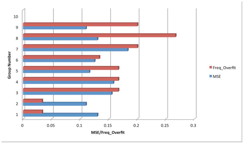
Trial-and-error process in selecting numbers of hidden neurons for a single layer (given splitting ratio: 75%:15%:15%). Group numbers 1–9 represent numbers of hidden neurons N = 4, 6, 8, 10, 12, 14, 16, 18, 20. The blue bar is the averaged value of MSE during a 30-cycle repetitive training process. The red bar represents the frequency where an overfitting problem occurs (Freq_Overfit) during the same training process.

Division of data

After we obtained the candidates (N = 4 and N = 6), the next step was to choose how to partition the data sets for training, validation, and testing. Once a splitting ratio is chosen, data points are selected randomly into the three subsets. Figure 3 demonstrates how a splitting ratio was determined by comparing MSE, Freq_Overfit, and Freq_Bad_Split_Indicator by using four (Fig. 3A) and six (Fig. 3B) hidden neurons. Freq_Overfit was defined as above and Freq_Bad_Split_Indicator was activated when the frequency of events where the test set error reaches a minimum occurs at a significantly different iteration step compared to the validation set. This is an indicator of a poor division of the data sets. Five different typical splitting ratios were chosen to test in this experiment. MSE is again an average value over 30 repetitions, excluding those with either an overfitting problem (Fig. 4A) or a bad splitting indication (Fig. 4B). Resampling techniques, such as k-fold cross-validation, are possible but unnecessary since each repetition uses random data to fill the partition sets. Finally, the relatively best splitting ratio was chosen for both cases (60%:25%:15%). However, because of a relatively better group performance, the neuron number N = 6 group was chosen for the real prediction task.

Figure 3.

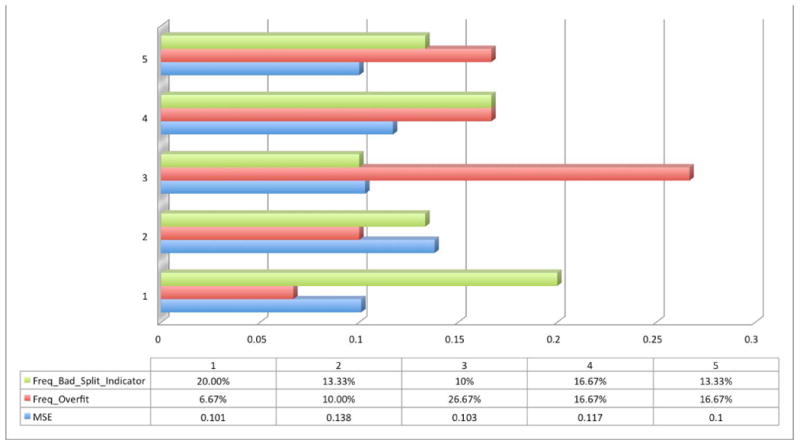
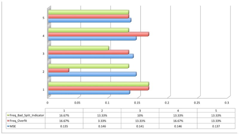
Trial-and-error process in selecting a specific splitting ratio for a network with four hidden neurons (A) and six hidden neurons (B). Group numbers 1–5 represent several common splitting ratios: 1 (50%:25%:25%), 2 (60%:25%:15%), 3 (60%:30%:10%), 4 (70%:15%:15%), and 5 (80%:10%:10%). The blue bar is the averaged value of MSE over a 30-cycle repetitive training process. The red bar represents the frequency where an overfitting problem occurs (Freq_Overfit) during the same training process. The green bar represents the frequency where a bad splitting indication (Freq_Bad_Split_Indicator) appears during the same training process.

Figure 4.

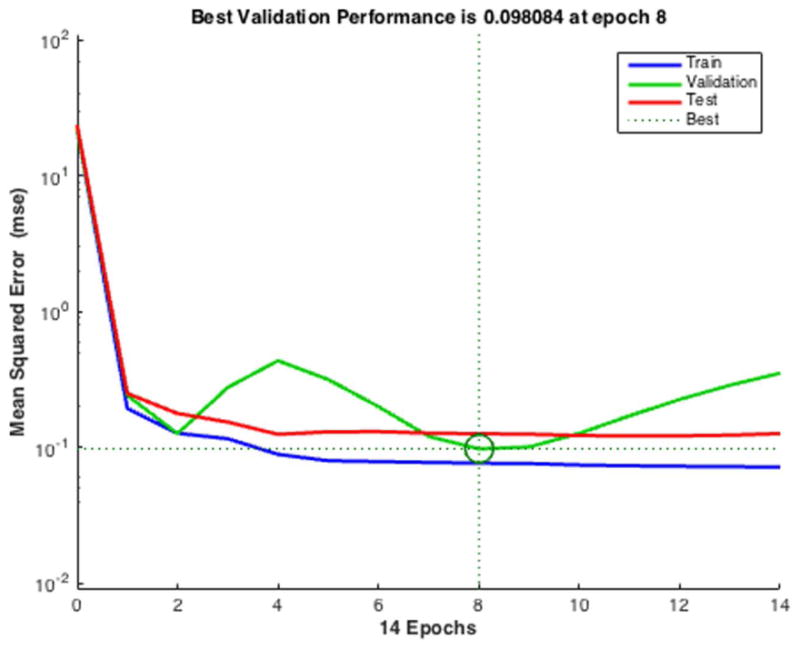
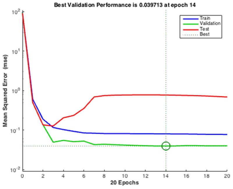
Example of poor evaluation results. (A) Overfitting errors rise as validation error increases before the best validation performance point (epoch 14). (B) Poor training results due to poor splitting ratio chosen: the smallest test error is located at a significantly different iteration (epoch 3) than the circled iteration (epoch 14).

For the ARMA comparison model, we also tested 10 different splitting ratios (see Appendix S1 (section II), Table S2, and Fig. S1 in Supporting Information online for a detailed description of this process); an 85%:15% splitting ratio was finally chosen.

After constructing the neural network and making the choice of data partitions, a model was built and ready to make predictions on the data, and we therefore proceeded to the model evaluation phase. To evaluate a model in machine learning, one needs to consider three steps: (1) determining whether, at the end of the learning iteration, a sufficiently small error (MSE) can be obtained in all three data sets (see validation results in Fig. 5); (2) checking whether any overfitting occurs (see validation results in Fig. 5); and (3) in addition to looking at MSE, plotting the model's output versus the real data (target data) characterizes the distribution of prediction error. The R-value of a subsequent regression tells us more about the model's predictive ability.

Figure 5.

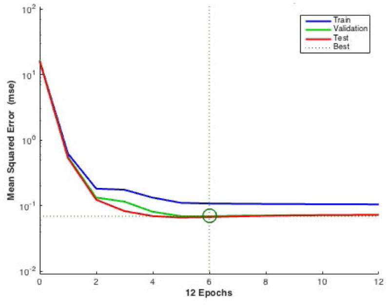
Performance of validation. The figure plots MSE versus the training epoch for all training (blue), validation (green), and test (red) data sets. The best validation performance point was circled in the figure (at epoch 6).

Validation analysis

The best validation results (with smallest validation error (MSE) at the circled iteration) are shown in Fig. 5 after 30 cycles of repetitive training. A well-trained ANN is shown here since it has a very low MSE (0.069) at the end of the training phase. No overfitting occured because testing and validation error were not rising before iteration 6.

Residual analysis

Residual plots are required for diagnostic checking, which will ensure the goodness of the forecasting model. The residuals (Fig. 6A, bottom panel) show random behavior and zero mean, indicating a lack of bias and confirming that forecasts are good. Histogram plots of the residuals (Fig. 6B) show an approximately normal distribution, satisfying a required assumption of the general ANN model. The residuals' autocorrelation function (ACF) plots (Fig. 6C) show that the errors do not possess significant correlations, which is important for good prediction. Residual analysis for ARMA is shown in Appendix S1 (section III) and Figure S2 in Supporting Information online.

Figure 6.

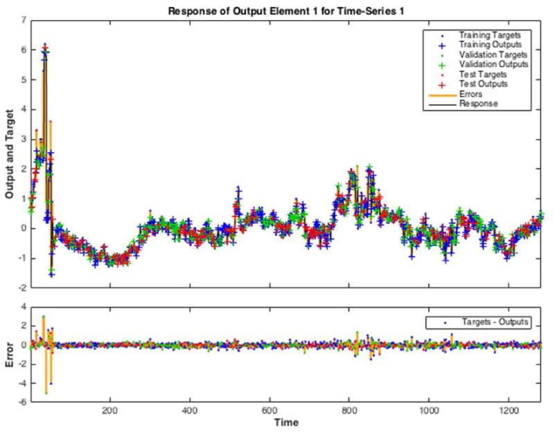
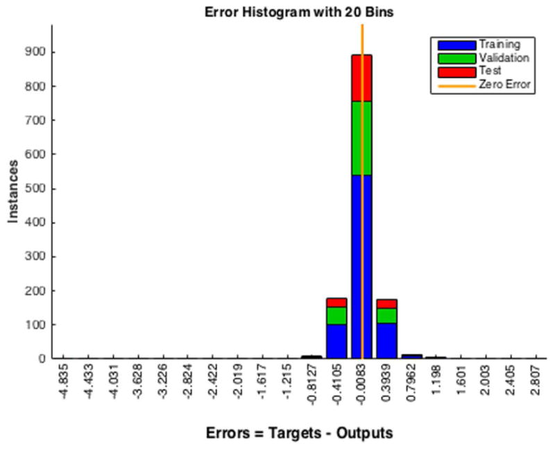
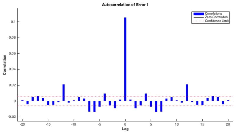
Residuals analysis for ANNs. (A) The output target response plot (top) shows how well the output (all three sets) fits the target. The residuals time series plot (bottom) shows no significant correlation and the mean of the residuals is very close to zero. (B) The residuals histogram plot (for all three sets) shows the normal distribution, which is compatible with the model assumption. (C) The residuals' ACF plot again shows a lack of correlation.

Regression analysis

Figure 7 shows output versus target of the ANN model together with a linear regression. These are the best that we could obtain after initiating the network and training over 30 repetitions. R values for all of the data sets exceeded 0.9, which indicates an accurate prediction. We observed that the predictive ability of the model is much better for values closer to the mean.

Figure 7.

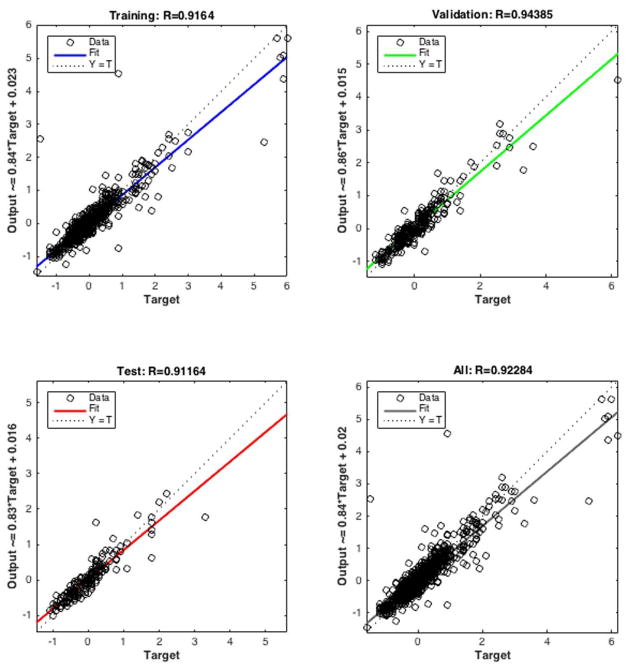
Regression plots. The three plots represent the regression relationships between prediction outputs and targets for (top left) training, (top right) validation, (bottom left) test, and all (bottom right) data sets. The dashed line in each plot represents the perfect result (outputs = targets). The solid line (blue for training, green for validation, red for test, and black for all) represents the best linear regression line between outputs and targets. The R value is an indication of the relationship between outputs and targets. R is between 0 (no linear relationship) and 1 (exact linear relationship).

Forecasting comparison

The mean MSE for both ANNs and ARMA is summarized in Table 1 for different splitting. The smallest MSE is around 0.5 for ARMA and around 0.1 for ANNs. Appendix S1 (section IV) and Fig. S3 in Supporting Information online show a visualization of prediction with ARMA. Although it shows a widely opened 95% confidence interval, the large MSE shows that ARMA cannot accurately predict the time series, which is the reason why we did not run the regression on residuals for ARMA. Overall, ANNs significantly outperform ARMA, as measured by prediction errors.

Table 1. Comparison of prediction results in ANNs and ARMA with different splitting ratios.

Split	75%: 25%	85%: 15%	90%: 10%	95%: 5%
MSE (ANN)	0.135	0.146	0.141	0.143
MSE (ARMA)	0.699	0.608	0.550	0.464

Note: ARMA's prediction is very sensitive to splitting ratios: the more training sets included, the more accurate it appears. ANNs' prediction is more robust (∼ 0.1) for all forecasting splitting. Note that because the error is as the same scale level of the real data, the mean value of MSE for both ANNs and ARMA can be compared without any scaling.

Discussion

This section is devoted to addressing several generally important issues on modeling dosimetry symmetry data and suggesting practical guidelines for future work.

Overfitting problems in ANNs

Overfitting is one of the most cited problems with ANNs: although the error in the training set is driven to a very small value, it cannot be generalized to fit the test data set. A suggested method for improving network generalization is to use a network that is just large enough to provide an adequate fit, because when the number of parameters in the network is much smaller than the total number of data points in the training set, there is little to no chance of overfitting.¹² The results shown in Fig. 2 illustrate the tradeoff process between reducing the size of the network (hence, avoiding the overfitting problem) and the need to maintain a low-level MSE. However, this process is laborious. Alternative methods, such as regularization and early stopping, are suggested and implemented in Neural Network Toolbox™ software. Fortunately, because of the large size of the training set (∼ 900 time steps), overfitting is less likely to happen and can be easily overcome by optimizing neuron network sizes; therefore, there is no need to address alternative techniques. However, in cases with a limited supply of data, these issues would become critical.

Partitioning the data

Splitting is a process that generally lacks strict guidelines. However, according to Zhang,¹³ “When the size of the available data set is large (e.g., more than 1000 observations), different splitting strategies may not have a major impact on adequate learning and evaluation.” But since time-series forecasting was found to cause more sample variation than the time-independent case, more attention should be drawn here, even with large data sets.

In general, splitting should be done randomly to make sure each subsample is representative of the population. Unfortunately, time-series data are often difficult to split randomly because of their natural ordered property. Systematic sampling has been suggested¹⁴ to be a more appropriate method in splitting naturally ordered datasets, such as time series.¹⁵ However, because of its relatively high computational cost and our relative non-sensitivity to data splitting (when large data sets are available), we decided to use a trial-and-error (generate-and-test) method, despite the drawback of being time consuming. Other partitioning strategies have been introduced^{14, 16} as well, but the main point is that a specific splitting strategy has to be tailored for each specific problem. Blindly using empirical rules or default settings regardless of the variation from one application to another should be avoided.

Comparison of ANNs with ARMA

From a practical point of view, ANNs are more valuable and advantageous for forecasting because of the following characteristics: (1) they are data-driven, directly learning from data or their experiences. This is particularly appropriate for our situation where the underlying data's generating mechanics are unknown and when large amounts of data are available for training and validation; and (2) from a theoretical point of view, ANNs are nonlinear models, whereas the ARMA has many restrictive assumptions, such as Gaussian distribution and linearity, which might not be applicable to our real-world time series. However, the overfitting problem tends to occur in ANNs more frequently than in ARMA.

Clinical significance/meanings

The behavior of our 5-year dosimetry data is very consistent with the seasonal fluctuation (quasi-periodic behavior) observed in previous studies,^{7, 17-20} particularly sinusoidal behavior. This is probably because of the combination of the air leakage of the over-pressurized sealed monitor chambers for the specific Linac vendor and environmental factors year-round, including the fixed timing of the startup of the air conditioning and heating in the facility. To our understanding, the stability of some Linac components can vary with seasonal temperature changes year-round and the incoming power to the main circuit board that affect the beam symmetry. This was evident in our symmetric plots for all energies observed with almost the same pattern (1 cycle = 12 months).⁷

Conclusions

These preliminary results show that ANNs have the potential for time-series prediction of dosimetric symmetry data and yield more powerful and accurate prediction results than does ARMA. We demonstrated its accurate validation performance; in our case, a simple small network (single layer and six neurons) can provide high quality in such a forecasting task. ANNs are completely data driven, which is especially useful for complex data of unknown nature. It is universally applicable and can be applied to almost any type of time-series patterns and is well-developed and simple to carry out. ANNs require no data preprocessing except for outlier correction and require no statistical test, making it a relatively realizable forecasting tool. Although the output drift would diminish after the first few years for a new Linac because of the gradually increased stability of the sealed monitor chambers, the results from this proof-of-principle study show the possibility of predicting certain Linac dosimetry trends using machine learning tools.

Supplementary Material

Supp Appendix S1

Supporting Information: Appendix S1. (I) Methods of ARMA modeling; (II) splitting ration selection for ARMA; (III) residual analysis for ARMA; and (IV) forecasting comparison.

Supp Fig S1

Figure S1. Mean prediction errors for different splitting ratio forecasted by ARMA. From left to right: splitting ratio = 1 (50%: 50%), 2 (55%: 45%), 3 (60%: 40%), 4 (65%: 35%), 5 (70%: 30%), 6 (75%: 25%), 7 (80%: 20%), 8 (85%: 15%), 9 (90%: 10%), and 10 (95%: 5%). As can be seen, the more data points that are included in the training set, the smaller the error will present.

Supp Fig S2

Figure S2. Residuals analysis for ARMA. The residuals time plot (upper left) shows randomness behavior and the mean is close to zero. The residuals histogram plot (upper right) shows the normal distribution, which is compatible with the model assumption. The residuals' ACF plot (bottom left) and partial autocorrelation function (PACF) plot (bottom right) again show the lack of correlation.

Supp Fig S3

Figure S3. Forecasting results from ARMA. The fitting is by using the first 85% of the observations. The evaluation (forecast) is on the last 15% of the observations.

Supp Table S1

Table S1. Bayesian information criteria (BIC) tests for ARMA (p = 1, 2, 3, 4; q = 1, 2, 3, 4). The row number indicate the degree of AR, which is denoted as p. The column number indicates the degree of MA, which is denoted as q. The best result (indicated in red) is the smallest BIC value: 701.2; it shows at p = 3 and q = 2.

Supp Table S2

Table S2. ARMA model parameter selection and prediction errors under different splitting. The first row is when spitting ratio = 1 (50%: 50%), 2 (55%: 45%), 3 (60%: 40%), 4 (65%: 35%), 5 (70%: 30%), 6 (75%: 25%), 7 (80%: 20%), 8 (85%: 15%), 9 (90%: 10%), and 10 (95%: 5%). The second row is the most appropriate parameter set that provides the smallest information criteria (BIC) value under each splitting. The third row shows the prediction error (MSE) under each splitting.

References

- 1.National Cancer Institute. http://www.cancer.gov/about-cancer/treatment/types/radiation-therapy/radiation-fact-sheet; publication date: June 30, 2010; last accessed date: July 26, 2016.
- 2.Hanson William F, et al. Physical Aspects of Quality Assurance in Radiation Therapy. AAPM 1994 [Google Scholar]
- 3.Yeung TK, et al. Quality assurance in radiotherapy: evaluation of errors and incidents recorded over a 10-year period. Radiother Oncol. 2005;74:283–291. doi: 10.1016/j.radonc.2004.12.003. [DOI] [PubMed] [Google Scholar]
- 4.Ishikura S. Quality assurance of radiotherapy in cancer treatment: toward improvement of patient safety and quality of care. Japanese journal of clinical oncology. 2008;38:723–729. doi: 10.1093/jjco/hyn112. [DOI] [PubMed] [Google Scholar]
- 5.Hunt MA, et al. The impact of new technologies on radiation oncology events and trends in the past decade: an institutional experience. International Journal of Radiation Oncology Biology Physics. 2012;84:925–931. doi: 10.1016/j.ijrobp.2012.01.042. [DOI] [PubMed] [Google Scholar]
- 6.Ford EC, et al. Quality control quantification (QCQ): a tool to measure the value of quality control checks in radiation oncology. International Journal of Radiation Oncology Biology Physics. 2012;84:e263–e269. doi: 10.1016/j.ijrobp.2012.04.036. [DOI] [PubMed] [Google Scholar]
- 7.Chan MF, et al. Visual Analysis of the Daily QA Results of Photon and Electron Beams of a Trilogy Linac over a Five-Year Period. International Journal of Medical Physics, Clinical Engineering and Radiation Oncology. 2015;04:290–299. doi: 10.4236/ijmpcero.2015.44035. [DOI] [PMC free article] [PubMed] [Google Scholar]
- 8.Adhikari R, Agrawal R. An introductory study on time series modeling and forecasting. 2013 arXiv preprint arXiv:1302.6613. [Google Scholar]
- 9.Frank RJ, Davey N, Hunt SP. Time series prediction and neural networks. Journal of intelligent and robotic systems. 2001;31:91–103. [Google Scholar]
- 10.Naqa IE, Li R, Murphy MJ. Machine Learning in Radiation Oncology: Theory and Applications. Springer International Publishing; 2015. [Google Scholar]
- 11.Valdes G, et al. A mathematical framework for virtual IMRT QA using machine learning. Medical physics. 2016;43(7):4323–4334. doi: 10.1118/1.4953835. [DOI] [PubMed] [Google Scholar]
- 12.Zhang G, Patuwo BE, Hu MY. Forecasting with artificial neural networks∷ The state of the art. International journal of forecasting. 1998;14:35–62. [Google Scholar]
- 13.Zhang GP. Avoiding pitfalls in neural network research. Systems, Man, and Cybernetics, Part C: Applications and Reviews. IEEE Transactions on. 2007;37:3–16. [Google Scholar]
- 14.Zhang GP, Berardi V. Time series forecasting with neural network ensembles: an application for exchange rate prediction. Journal of the Operational Research Society. 2001;52:652–664. [Google Scholar]
- 15.Taskaya-Temizel T, Casey MC. A comparative study of autoregressive neural network hybrids. Neural Networks. 2005;18:781–789. doi: 10.1016/j.neunet.2005.06.003. [DOI] [PubMed] [Google Scholar]
- 16.Reitermanova Z. Data splitting. WDS's 10 proceedings of contributed papers, Part. 2010;1:31–36. [Google Scholar]
- 17.Grattan M, Hounsell A. Analysis of output trends from Varian 2100C/D and 600C/D accelerators. Physics in medicine and biology. 2010;56:N11. doi: 10.1088/0031-9155/56/1/N02. [DOI] [PubMed] [Google Scholar]
- 18.Bartolac S, Letourneau D. SU-ET-136: Assessment of Seasonal Linear Accelerator Output Variations and Associated Impacts. Medical physics. 2015;42:3363–3363. [Google Scholar]
- 19.Hossain M. Output trends, characteristics, and measurements of three mega-voltage radiotherapy linear accelerators. Journal of applied clinical medical physics/American College of Medical Physics. 2014;15:4783. doi: 10.1120/jacmp.v15i4.4783. [DOI] [PMC free article] [PubMed] [Google Scholar]
- 20.Uddin MT. Proceedings of IPAC2012. New Orleans: 2012. Quality Control of Modern Linear Accelerator: Dose Stability Long and Short-Term. [Google Scholar]
Associated Data
This section collects any data citations, data availability statements, or supplementary materials included in this article.
Supplementary Materials