Abstract
Measuring multidimensional (e.g., 2D) relaxation spectra in NMR and MRI clinical applications is a holy grail of the porous media and biomedical MR communities. The main bottleneck is the inversion of Fredholm integrals of the first kind, an ill-conditioned problem requiring large amounts of data to stabilize a solution. We suggest a novel experimental design and processing framework to accelerate and improve the reconstruction of such 2D spectra that uses a priori information from the 1D projections of spectra, or marginal distributions. These 1D marginal distributions provide powerful constraints when 2D spectra are reconstructed, and their estimation requires an order of magnitude less data than a conventional 2D approach. This marginal distributions constrained optimization (MADCO) methodology is demonstrated here with a polyvinylpyrrolidone-water phantom that has 3 distinct peaks in the 2D D-T1 space. The stability, sensitivity to experimental parameters, and accuracy of this new approach are compared with conventional methods by serially subsampling the full data set. While the conventional, unconstrained approach performed poorly, the new method had proven to be highly accurate and robust, only requiring a fraction of the data. Additionally, synthetic T1-T2 data are presented to explore the effects of noise on the estimations, and the performance of the proposed method with a smooth and realistic 2D spectrum. The proposed framework is quite general and can also be used with a variety of 2D MRI experiments (D-T2, T1-T2, D-D, etc.), making these potentially feasible for preclinical and even clinical applications for the first time.
Keywords: Fredholm integral, Inverse problems, Relaxometry, Diffusometry, Reconstruction, Multidimensional, Distribution
1. Introduction
Multidimensional NMR experiments allow us to study correlations between relaxation properties, such as T1 and T2, and physical parameters, such as the diffusivity (D). These correlations can be used to identify and characterize microstructure-related water dynamics in many applications [1–3]. The following general expression [4] describes the signal attenuation from 2D NMR experiments with separable kernels:
| (1) |
β1 and β2 are experimental parameters that are determined by the data acquisition scheme, and ω1 and ω2 are the relaxation/diffusion variables. Eq. (1) is an example of a broad class of Fredholm integrals of the first kind. When the kernels have an exponential form, application of a 2D inverse Laplace transform (ILT), which is a classic ill-conditioned problem [5], is required. The most common and efficient 2D-ILT algorithm [6] is typically used in 2D relaxometry experiments that involve a Carr-Purcell-Meiboom-Gill (CPMG) acquisition, which results in high density sampling of the signal decay. This algorithm greatly improved the efficiency of the inversion by compressing the 2D signal without losing useful information, revealing a redundancy in some basis representations.
Although multidimensional diffusion/relaxation experiments have been of great interest in recent years, preclinical and clinical applications are infeasible. In high-field 3 T and 7 T MRI scanners, the total number of 180° pulses that can be applied per unit time is limited by safety concerns, primarily due to the high specific absorption rate (SAR) [7]. Fast spin-echo, multi-echo, or CPMG pulse trains are therefore not clinically applicable, and the large amounts of data required cannot be collected in in vivo experiments due to long scan times. Each acquisition – whether D-T1 or, for example, T1-T2 measurements absent a CPMG pulse train – would only result in a single experimental data point. An additional experiment where the 2D data surface is sampled point by point is the diffusion–diffusion exchange spectroscopy (DEXSY) [2]. When a potentially lengthy imaging block is added, shortening the scan time becomes the primary challenge.
The goal of this work is to vastly reduce the number of acquisitions required for an accurate 2D diffusion/relaxation spectrum reconstruction. Recently, a strategy was introduced that used the marginal 1D distributions of a joint diameter-length distribution of a porous material comprised of capped (finite) cylinders as equality constraints to stabilize and reduce the number of acquisitions needed to invert a discrete Fredholm equation [8]. Applying the concept of marginal distributions constrained optimization (MADCO) to 2D relaxometry/diffusometry NMR, we note that the 1D projections of a 2D correlation function of two relaxation/diffusion parameters are directly related to it, and if obtained a priori, can be used to greatly constrain the solutions space of F(ω1,ω2).
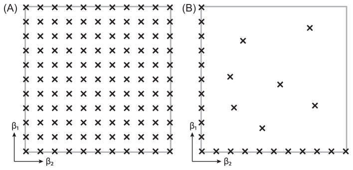
We suggest here a novel experimental design and reconstruction framework: instead of sampling the entire experimental parameters space, (β1, β2), and directly estimate the 2D distribution F(ω1,ω2) (Fig. 1A), using MADCO would only require sampling along β1 and β2 axes (i.e., 1D data), complemented with a small number of acquisitions in the 2D space (Fig. 1B). The 2D reconstruction would then have two steps: (1) estimate F(ω1) and F(ω2) from the 1D data, and then (2) use these 1D spectra to constrain the estimation of F(ω1,ω2) from the remaining 2D data.
Fig. 1.
Illustration of the (A) conventional and (B) MADCO experimental design schemes used to obtain a 2D correlation function, F(ω1,ω2).
Although the method is equally applicable to other types of multidimensional experiments, we chose to demonstrate it experimentally on a D-T1 polyvinylpyrrolidone (PVP) water solution phantom. A clinically applicable inversion recovery diffusion-weighted imaging pulse sequence was used to observe D-T1 correlations. Additionally, synthetic T1-T2 data are presented to explore the effects of noise on the estimations, and the performance of the proposed method with a smooth and realistic 2D spectrum. The suggested and the conventional established methods were investigated to determine the generalizability of our analyses.
2. Experiments
2.1. D-T1 phantom preparation and data acquisition
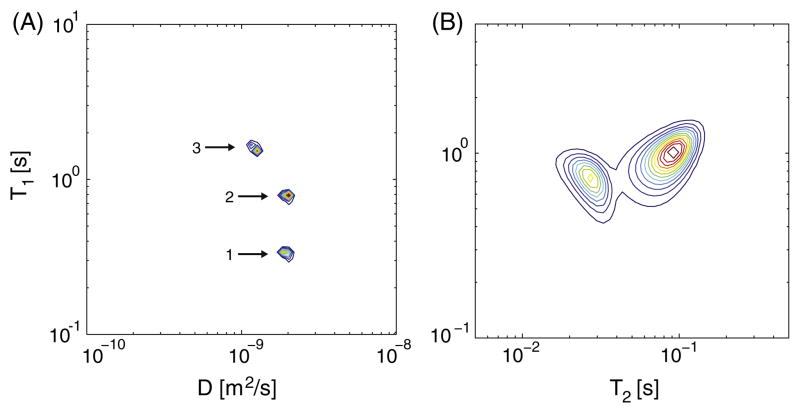
Doped water and PVP (Sigma-Aldrich, K value 29–32) were used to create a D-T1 phantom with three distinct peaks. Aqueous solutions of PVP were shown to make good diffusion MR phantoms since their measured diffusivity is independent of the diffusion time, indicating Gaussian diffusion of a single population of spins [9]. In addition, increasing PVP w/v concentration is negatively correlated with both the diffusivity and T1. Two purified water samples with 0.18 mM and 0.5 mM gadopentetate dimeglumine (Magnevist, Bayer, Germany) were prepared, along with a 20% w/v PVP water solution sample. The corresponding weighted geometric means (gm) of the relaxation times and diffusivities (gmT1, gmD), as measured separately for each sample (see Section 3) are shown in Fig. 2A. Each sample was placed in a 4 mmNMR tube; these were then inserted together into a 15 mm NMR tube.
Fig. 2.
(A) Ground truth T1-D distribution obtained from a separate analysis of each (T1,D) sample and averaging according to the relative spin density. The 3 peaks are identified and numbered for future reference, and their (gmT1, gmD) values were 1. (293 ms, 2.26 μm2/ms), 2. (782 ms, 1.99 μm2/ms), and 3. (1596 ms, 1.24 μm2/ms). (B) T1-T2 relaxometry of the simulated ground truth, with peaks centers (T1, T2) at (921 ms, 27.1 ms) and (1013 ms, 73.6 ms).
Imaging data were collected on a 7 T Bruker wide-bore vertical magnet with an AVANCE III MRI spectrometer equipped with a Micro 2.5 microimaging probe. MRI data were acquired with an inversion recovery spin-echo diffusion-weighted echo planar imaging (IR–DWI–EPI) sequence, with an adiabatic 180° inversion pulse applied before the standard spin-echo diffusion weighted sequence. The full 2D experimental set had 40 diffusion gradient linear steps (G) ranging from 0 to 900 mT/m, 37 inversion times (τ1) with logarithmic temporal spacing ranging from 100 to 3000 ms, and an additional magnetization equilibrium scan with an inversion time of 10 s. The 1D experiments were a subset of the full 2D data set. The 1D IR data set included all of the 37 inversion times with G = 0, and the 1D diffusion data set included all of the odd diffusion gradient linear steps (total of 20) with τ1 = 10 s. Other acquisition parameters were diffusion gradient duration and separation of δ = 3 ms and Δ = 15 ms, respectively, leading to a b-value range of 0–6200 s/mm2 (b = γ2δ2G2(Δ − δ/3), where γ is the gyromagnetic ratio), TE = 50 ms, and TR = inversion time + 10 s. A single 5 mm axial slice with a matrix size and resolution of 64 × 64 and 0.2 × 0.2mm2, respectively, acquired with 2 averages and 4 segments. The experimental signal-to-noise ratio (SNR) in the full 2D experiment was ~700.
2.2. Simulations
Two peaks in a 2D T1-T2 relaxogram with positions and patterns similar to those obtained from spinal cord white matter [10,11] were used as the joint distribution (Fig. 2B) to generate the data using the T1 and T2 kernels, with Gaussian noise at low and high SNRs of 200 and 2500, respectively. For each SNR value, 200 realizations of noisy data were generated and from each of these 1D T1 and T2 spectra, and 2D T1-T2 spectrum were fitted using the procedure described in Section 3, and subsequently averaged. The number of acquisitions that considered a ‘‘full sample” was based on previous studies [12,13], and was set at 30 logarithmically distributed inversion times, τ1, ranging from 200 to 4000 ms, and 1024 logarithmically distributed echo times, τ2, ranging from 5 to 200 ms (total of 30,720).
3. Methods
Eq. (1) can be discretized with Nω1 and Nω2 values of ω1 and ω2, respectively, and Nβ1 and Nβ2 values of β1 and β2, respectively, and have the general form of
| (2) |
The specific kernels that were used in this study were
| (3a) |
| (3b) |
| (3c) |
while it is worth noting that for T1-weighted measurements the fully recovered data are subtracted from the data set to remove signal offset. When the kernels are separable, a 2D kernel can be defined as the product K(ω1, β1,ω2, β2) = K1(ω1, β1)K2(ω2, β2), and Eq. (2) can be written in matrix form as
| (4) |
where M and F are (Nβ1Nβ2) × 1 and (Nω1Nω2) × 1 vectors, and K is a (Nβ1Nβ2) × (Nω1Nω2 ) matrix. As discussed earlier, Eq. (4) represents an ill-conditioned problem, i.e., a small change in M may result in large variations in F. A standard approach to solving ill-conditioned problems is to regularize them. When the spectrum is expected to be smooth, ℓ2 regularization is appropriate [14], and therefore was used in the T1-T2 distribution simulations. However, in the case of the phantom, the D-T1 space is comprised of discrete components, therefore making ℓ1 regularization a more suitable choice since it has many of the beneficial properties of ℓ2 regularization, but yields sparse models [15]. The regularized problem considered in this study was
| (5) |
where||···||i are the ℓ1 and ℓ2 norms, for i = 1, 2, respectively. The regularization parameter, α, was chosen based on the S-curve method [14], which uses the fit error, χ(α) = ||KF(α) − M||2. The regularization parameter was determined such that d(log χ)/d(log α) = TOL, with TOL = 0.1 [14].
In this work we suggest a simple way to stabilize the solution of Eq. (5), while significantly reducing the number of required acquisitions (i.e., Nβ1 and Nβ2) and improving accuracy. Since F(ω1,ω2) is in fact the joint distribution of ω1 and ω2, it is related to the 1D marginal distributions F(ω1) and F(ω2) by
| (6) |
These marginal distributions, however, can be separately estimated from 1D experiments, and then used to find F(ω1,ω2) by applying the two parts of Eq. (6) as equality constraints when Eq. (5) is solved. The 1D problems, in which Eq. (5) is solved by replacing the (Nβ1Nβ2) × (Nω1Nω2 ) kernel K with kernel K1 or kernel K2 ( and are the number of 1D acquisitions), reduce the number of free parameters by a factor of Nω2 and Nω1, respectively. Using MADCO will be shown here to dramatically reduce the number of acquisitions required to estimate the 2D distribution, such that and . The 1D estimation suffers from the same ill-posed nature of the 2D case, and therefore these equality constraints should be relaxed in the presence of experimental noise, when the estimation of F(ω1) and F(ω2) is expected to be inaccurate. In this case the constraints are
| (7) |
and
| (8) |
where in this work σ was set as the standard deviation (SD) of the noise (as determined after complete signal decay) normalized by the unattenuated signal. It is worth noting that while the constraints in Eq. (6) have a deductive value, Eqs. (7) and (8) should be used when processing noisy data. Similarly to the standard non negativity constraints, the inequality constraints in Eqs. (7) and (8) also represent physical conditions that must be fulfilled (‘‘conservation of mass” of the 2D probability distribution projected onto one of its axes), and can be applied in a similar manner.
Performance of the proposed method was assessed by computing the Jensen difference, which is a well-established method of measuring distance between two probability distributions [16]. The Jensen difference metric is a symmetric version of the Kullback-Leibler divergence that is bounded by 0 and 1 and is defined for two distributions, Q and P, as
| (9) |
4. Results
4.1. D-T1 distribution PVP phantom
In the phantom study, NT1 = ND = 50, , and the number of 2D experiments (Nτ1Nb) were varied in the range of 7–1480, while stability and accuracy were quantified. Imaging the PVP phantom enabled separate analysis of each of the (T1,D) samples by the selection of 3 ROIs. For each ROI, separately solving Eq. (5) with the kernels KD and KT1 , using the full 2D data set and the 1D subsets resulted in estimations of FGT (T1,D), FGT (T1), and FGT (D) (GT stands for ground truth). Estimating the spectra of single peak data (i.e., monoexponential) is a well-posed problem, and therefore the 1D and 2D distributions obtained from these analyses were averaged according to their relative spin density and taken as the ground truth (Fig. 2A for D, and Fig. 1S in the SI for 1D).
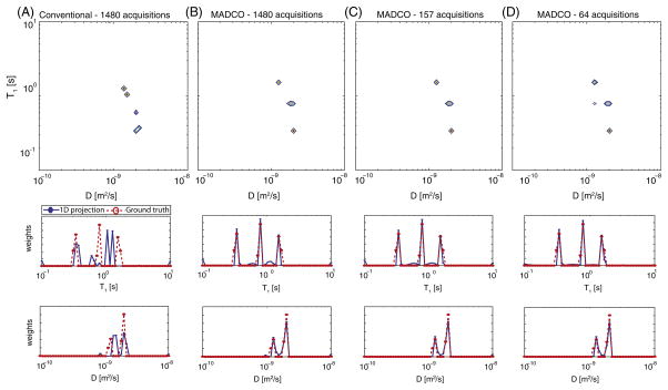
The performance of MADCO was determined and compared with the conventional method by estimating the D-T1 distribution by using 500 random subsamples from the full data at 19 logarithmically distributed number of acquisitions. Two-dimensional distribution reconstruction and its 1D projections using the conventional experimental design (Fig. 1A) when the full data set is used (1480 acquisitions) are shown in Fig. 3A (similarly, results using 2 more data subsamples – 64, 157 acquisitions – are shown in Fig. 2S in the SI). Visually compared with the ground truth in Fig. 2A, the estimated results in Fig. 3A are inaccurate, both for the 2D and 1D projections.
Fig. 3.
D-T1 phantom spectra reconstruction using the two methods. (A) Conventional approach using the full data set. MADCO approach using (B) the full data set, and subsamples of (C) 157 acquisitions, and (D) 64 acquisitions. The 1D projections (blue circles) overlaid with the ground truth 1D distributions (red circles) are presented below each 2D spectrum. (For interpretation of the references to color in this figure legend, the reader is referred to the web version of this article.)
Spectra reconstructed using the MADCO experimental design (Fig. 1B) and processing framework at 3 representative data subsamples – 64, 157, and 1480 acquisitions (7, 100, and 1423 2D acquisitions along with 20 and 37 1D diffusion and IR acquisitions, respectively) are shown in Fig. 3B–D. Stability, as well as accuracy, are evident from the 2D distributions, in which little to no difference was noted as the number of acquisitions was decreased by a factor of 25. In terms of establishing the peaks (mean and amplitude) accuracy, MADCO outperformed the conventional method in almost every instance, while consistently keeping the normalized root mean square error well-below 10%. (For the complete list of parameters and details regarding the error computation, please refer to the SI.)
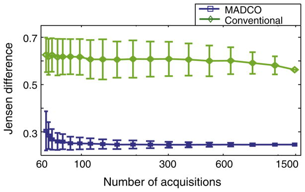
As opposed to first and second moment parameters accuracy, it is more informative to study the accuracy of the entire reconstructed 2D distribution as a function of the number of acquisitions. Jensen differences between the estimated and the ground truth distributions were calculated after reconstruction of the 2D distributions with and without MADCO. For each number of acquisitions, averages and SDs of the 2D Jensen differences from the 500 random subsamples were computed and are presented in Fig. 4. The high accuracy of MADCO reconstruction is demonstrated by its markedly low Jensen difference from the ground truth, compared with results from the unconstrained approach. The stability of MADCO is evident from the relatively small SD and its low variability. Conversely, the conventional method resulted in large SD that points to a high degree of sensitivity to experimental parameters, which was mitigated by using MADCO.
Fig. 4.
Accuracy and stability of the methods demonstrated by the Jensen differences between the estimated and the ground truth distributions, with the conventional (green diamonds) and MADCO (blue squares) methods, as a function of the number of acquisitions. (For interpretation of the references to color in this figure legend, the reader is referred to the web version of this article.)
4.2. T1-T2 distribution simulations
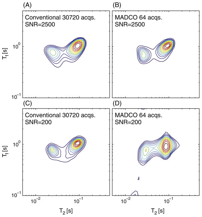
Computer simulation data are presented to address three issues relevant to this work: (1) evaluate the performance of the proposed method with a smooth and continuous 2D spectrum, (2) demonstrate the T1-T2 correlation case, and (3) examine how the SNR affects the estimation. In the simulations study, NT1 = NT2 = 50, , along with 4 additional 2D acquisitions for the MADCO approach (total of 64 acquisitions). The number of acquisitions for the conventional approach was Nτ1 = 30, and Nτ2 = 1024, a total of 30,720 2D acquisitions.
After experimentally establishing a high degree of accuracy at a moderate SNR (700), simulations were used to explore very high and very low SNR levels. For the full data with noise at SNR = 2500, the conventional approach yielded a close estimate (Fig. 5A) of the ground truth (Fig. 2B) with a Jensen distance of 0.018. At the same high SNR, the MADCO approach resulted in a highly accurate estimate as well (Jensen distance of 0.023, Fig. 5B), while using 480 times less data. Using both approaches, the estimated 2D distributions resembled the ground truth both in the shape and orientation of the peaks, and their location and amplitude.
Fig. 5.
T1-T2 simulations spectra reconstruction using the two methods. Conventional approach using the full data set with noise at (A) SNR = 2500, and (C) SNR = 200. MADCO approach using 64 acquisitions with noise at (B) SNR = 2500, and (D) SNR = 200.
Although less accurate, the estimated spectrum at the low SNR level (SNR = 200) with the conventional approach using the full data (Fig. 5C) was still fairly close to the ground truth, with a Jensen distance of 0.021. This time the accuracy of the contour of the peaks was reduced, while their location preserved. Using 64 acquisitions at an SNR of 200 with the MADCO approach resulted in a reasonable reconstruction, with a Jensen distance of 0.094 (Fig. 5D). While both peaks were resolved with accurate locations and amplitudes, their shape and orientation did not perfectly match the ground truth.
5. Discussion
Despite the ill-conditioned nature of the numerical inversion of the Fredholm integrals of the first kind, this problem is at the heart of many applications [1,3,13,17]. The resultant data bottleneck that require a large number of experiments and samples has made many applications impractical or infeasible. For example, although 2D NMR experiments are very powerful, because of the long acquisition time required to obtain sufficient data to invert the Fredholm equation, these experiments have not been migrated to in vivo preclinical or clinical MRI applications. In this work we have suggested a novel framework to stabilize, accelerate, and improve the reconstruction of a 2D spectrum by using the more easily accessible knowledge about its 1D projections. MADCO is a general mathematical approach for improving the properties of ILT and has been demonstrated here experimentally on a D-T1 phantom sample comprised of 3 distinct peaks, and on a simulated smooth T1-T2 distribution. Our results showed that, provided a reasonably accurate estimation of the 1D marginal distributions, constraining Eq. (5) with the inequalities in Eqs. (7) and (8) resulted in a high level of accuracy while using a fraction of the full data set. The efficiency of the proposed method can be expressed by considering the number of dimensions, 𝒩, and the number of acquisitions required to reconstruct the 1D spectrum in a given dimension, M. The conventional approach would require 𝒪(M𝒩) measurements, while using MADCO only 𝒪(M𝒩) acquisitions are needed.
In the experiments on the D-T1 distribution PVP phantom, the full acquisition scan time was ~37 h. As shown, the D-T1 distribution estimated using the conventional method was far from accurate, even when the full data set was used. Conversely, applying the proposed method led to very good agreement with the ground truth distribution, even when using only 4% of the full data set (64 acquisitions). It is fair to assume that additional acquisitions would have improved the accuracy of the conventional approach (leading to a convergence in the Jensen distance in Fig. 4). Since such a convergence could not be reached because of practical considerations, it is difficult to establish the true acceleration factor of MADCO based on the D-T1 experiment (although it is guaranteed to be greater than 1480/64 ≈ 25).
The T1-T2 distribution simulations study allowed to examine some aspects that the PVP phantom experiment could not determine, which were mainly the effects of noise on the estimations, and the performance of the proposed method with a smooth and realistic 2D spectrum. The simulations showed that in the case of high SNR data, the resulting T1-T2 spectra obtained using the conventional and the proposed approaches were quantitatively and qualitatively comparable. Both estimates were highly accurate, only that the MADCO approach used 480 times less data. When high levels of noise were introduced, the conventional approach yielded a more accurate 2D spectrum, especially in terms of the general shape and contour of the peaks. While the MADCO approach was able to resolve the two peaks, their locations, amplitude, and spread with high accuracy, their shape was not well preserved. According to this analysis, if the exact shape of the peaks in the 2D spectrum is of importance, SNR should be in the order of 700 (the SNR level in the D-T1 PVP phantom experiment). Even though an SNR of 700 in a 2D relaxometry in vivo MRI acquisition is feasible, the exact shape of the peaks may not be crucial in many applications, in which case an SNR of 200 and an order of 65 acquisitions should suffice.
With the imaging parameters that were used in the phantom study 64 acquisitions, corresponding to ~90 min in scan time, were sufficient for a complete and accurate D-T1 distribution mapping using the proposed method. Although this is a phantom study, we intentionally used an IR–DWI–EPI pulse sequence, which can be directly applied to in vivo preclinical and clinical studies. The conservatively chosen repetition time in this study could have been reduced from 10 s to the widely used range in in vivo T1 mapping applications of ~3 s [18], resulting in a total acquisition time of ~30 min. Further acceleration can be achieved by using a version of the Look-Locker acquisition for T1-weighting [19]. Recent advances in sampling strategies, such as compressed sensing for relaxometry parameter space [11], may be integrated with the MADCO method to increase the 2D acquisition efficiency.
Among other biological applications, characterization of nerve tissue with 2D diffusometry/relaxometry MRI may be able to reveal otherwise inaccessible information. Preliminary findings from 2D MRI experiments on nerve tissue analyzed with MADCO by our group indicate sensitivity to microstructural features and complex water exchange dynamics (data not shown). Future work could provide a comprehensive investigation in a reasonable time frame by using the method in conjunction with a variety of 2D experiments, such as D-T2 and T1-T2 correlation and T2-T2 and D-D exchange studies. Furthermore, our work may be extended beyond 2D, since application of the marginal distributions constrained optimization principle in higher dimensions enables the main limitation of experimental time to be lifted.
Supplementary Material
Acknowledgments
This work was supported by funds provided by the Intramural Research Program of The Eunice Kennedy Shriver National Institute of Child Health and Human Development (NICHD). The authors thank Dr. Martin Lizak for writing the IR-DWI pulse sequence, Dr. Jian Cheng for providing fruitful discussions, and Ms. Liz Salak for editing the manuscript.
Appendix A. Supplementary material
Supplementary data associated with this article can be found, in the online version, at http://dx.doi.org/10.1016/j.jmr.2016.08.004.
References
- 1.Does MD, Gore JC. Compartmental study of T1 and T2 in rat brain and trigeminal nerve in vivo. Magn Reson Med. 2002;47:274–283. doi: 10.1002/mrm.10060. [DOI] [PubMed] [Google Scholar]
- 2.Callaghan PT, Furó I. Diffusion-diffusion correlation and exchange as a signature for local order and dynamics. J Chem Phys. 2004;120:4032. doi: 10.1063/1.1642604. [DOI] [PubMed] [Google Scholar]
- 3.Hürlimann MD, Burcaw L, Song YQ. Quantitative characterization of food products by two-dimensional D-T2 and T1-T2 distribution functions in a static gradient. J Colloid Interface Sci. 2006;297:303–311. doi: 10.1016/j.jcis.2005.10.047. [DOI] [PubMed] [Google Scholar]
- 4.English AE, Whittall KP, Joy MLG, Henkelman RM. Quantitative two-dimensional time correlation relaxometry. Magn Reson Med. 1991;22:425– 434. doi: 10.1002/mrm.1910220250. [DOI] [PubMed] [Google Scholar]
- 5.McWhirter JG, Pike ER. On the numerical inversion of the Laplace transform and similar Fredholm integral equations of the first kind. J Phys A: Math Gen. 1978;11:1729–1745. [Google Scholar]
- 6.Venkataramanan L, Song Yi-Qiao, Hurlimann M. Solving Fredholm integrals of the first kind with tensor product structure in 2 and 2.5 dimensions. IEEE Trans Signal Process. 2002;50:1017–1026. [Google Scholar]
- 7.Shellock FG. Radiofrequency energy-induced heating during MR procedures: a review. J Magn Reson Imaging. 2000;12:30–36. doi: 10.1002/1522-2586(200007)12:1<30::aid-jmri4>3.0.co;2-s. [DOI] [PubMed] [Google Scholar]
- 8.Benjamini D, Basser PJ. Joint radius-length distribution as a measure of anisotropic pore eccentricity: an experimental and analytical framework. J Chem Phys. 2014;141:214202. doi: 10.1063/1.4901134. [DOI] [PMC free article] [PubMed] [Google Scholar]
- 9.Pierpaoli C, Sarlls J, Nevo U, Basser P, Horkay F. Polyvinylpyrrolidone (PVP) water solutions as isotropic phantoms for diffusion MRI studies. Proceedings of the 17th Annual Meeting of ISMRM; Honolulu, HI, USA. 2009. [Google Scholar]
- 10.Harrison R, Bronskill MJ, Henkelman RM. Magnetization transfer and T2 relaxation components in tissue. Magn Reson Med. 1995;33:490–496. doi: 10.1002/mrm.1910330406. [DOI] [PubMed] [Google Scholar]
- 11.Bai R, Cloninger A, Czaja W, Basser PJ. Efficient 2D MRI relaxometry using compressed sensing. J Magn Reson. 2015;255:88–99. doi: 10.1016/j.jmr.2015.04.002. [DOI] [PubMed] [Google Scholar]
- 12.Does MD, Beaulieu C, Allen PS, Snyder RE. Multi-component T1 relaxation and magnetisation transfer in peripheral nerve. Magn Reson Imaging. 1998;16:1033–1041. doi: 10.1016/s0730-725x(98)00139-8. [DOI] [PubMed] [Google Scholar]
- 13.Song YQ, Venkataramanan L, Hürlimann M, Flaum M, Frulla P, Straley C. T1-T2 correlation spectra obtained using a fast two-dimensional Laplace inversion. J Magn Reson. 2002;154:261–268. doi: 10.1006/jmre.2001.2474. [DOI] [PubMed] [Google Scholar]
- 14.Fordham E, Sezginer A, Hall L. Imaging multiexponential relaxation in the (y, LogeT1) plane, with application to clay filtration in rock cores. J Magn Reson Ser A. 1995;113:139–150. [Google Scholar]
- 15.Tibshirani R. Regression shrinkage and selection via the lasso. J Roy Stat Soc Ser B (Methodol) 1996;58:267–288. [Google Scholar]
- 16.Endres D, Schindelin J. A new metric for probability distributions. IEEE Trans Inform Theory. 2003;49:1858–1860. [Google Scholar]
- 17.Benjamini D, Nevo U. Estimation of pore size distribution using concentric double pulsed-field gradient NMR. J Magn Reson. 2013;230:198–204. doi: 10.1016/j.jmr.2013.03.001. [DOI] [PubMed] [Google Scholar]
- 18.Mulkern RV, Zengingonul HP, Robertson RL, Bogner P, Zou KH, Gudbjartsson H, Guttmann CR, Holtzman D, Kyriakos W, Jolesz FA, Maier SE. Multi-component apparent diffusion coefficients in human brain: relationship to spin-lattice relaxation. Magn Reson Med. 2000;44:292–300. doi: 10.1002/1522-2594(200008)44:2<292::aid-mrm17>3.0.co;2-q. [DOI] [PubMed] [Google Scholar]
- 19.Look DC, Locker DR. Time saving in measurement of NMR and EPR relaxation times. Rev Sci Instrum. 1970;41:250. [Google Scholar]
Associated Data
This section collects any data citations, data availability statements, or supplementary materials included in this article.


