Multiple Hypotheses Image Segmentation and Classification With Application to Dietary Assessment

Abstract

We propose a method for dietary assessment to automatically identify and locate food in a variety of images captured during controlled and natural eating events. Two concepts are combined to achieve this: a set of segmented objects can be partitioned into perceptually similar object classes based on global and local features; and perceptually similar object classes can be used to assess the accuracy of image segmentation. These ideas are implemented by generating multiple segmentations of an image to select stable segmentations based on the classifier’s confidence score assigned to each segmented image region. Automatic segmented regions are classified using a multichannel feature classification system. For each segmented region, multiple feature spaces are formed. Feature vectors in each of the feature spaces are individually classified. The final decision is obtained by combining class decisions from individual feature spaces using decision rules. We show improved accuracy of segmenting food images with classifier feedback.

I. Introduction

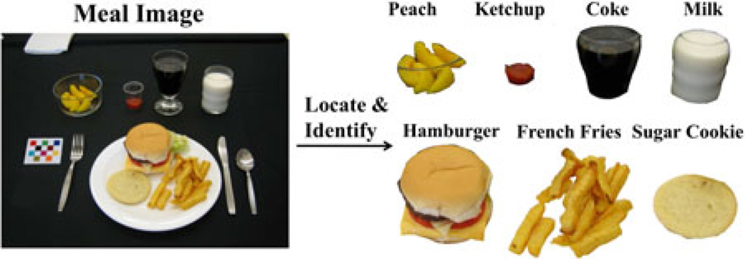
We are interested in developing methods to locate and identify perceptually similar food objects in an image for dietary assessment applications. Accurate assessment of food and beverage intake is an open problem in the nutrition field [1]. Our research focuses on developing a food record method using a mobile device that will provide an accurate account of daily food and nutrient intake [2]. Our goal is to identify food items using a single image acquired from the mobile device (e.g., a mobile telephone). An example of this is shown in Fig. 1, where each food item is segmented and identified. Our proposed dietary assessment system consists of two main parts: a mobile application and a “backend” system consisting of a computation server and a database system. In our system, images captured by users “before” and “after” eating occasions are sent to the server for automatic image analysis. Results are sent back to the mobile device for confirmation and review. None of the image analysis/classification described in this paper is done on the mobile device. It is all done on the server. The overall system and its applications are described in more detail in our previous paper [2].

Fig. 1.

Ideal food image analysis system.

Assigning class labels to every pixel in an image is a highly unconstrained problem, yet the human vision system is able to group pixels of an image into meaningful object segments without knowing a priori what objects are present in the image. Designing systems capable of making more informed decisions based on increased spatial information is an open problem for image segmentation and classification. It is necessary to work at different spatial scales on segmented regions that can model either entire objects, or at least sufficiently distinct parts of them. In [3], a framework for generating and ranking plausible objects hypotheses by solving a sequence of constrained parametric min-cut problems and ranking the object hypotheses based on mid-level properties is presented. A multiple hypotheses framework is proposed in [4] for robust estimation of the scene structure from a single image and obtaining confidences for each geometric label. Sivic et al. [5] used a probability latent semantic analysis model to determine the object categories in a set of unlabeled images.

Schemes for object classification usually proceed in two stages. First, features of the object or segmented region are measured or “extracted” and then the features are classified to obtain a decision regarding which class label to assign to a particular object [6]. An essential step is to adequately represent the information of the object by the features. The goal is to find features that can efficiently distinguish between objects belonging to different classes (interclass discrimination), and also describe as much information as possible for one class so that two objects of the same class, with different properties, can be classified together (intraclass robustness). Once the features for each object are obtained, a classification system selects the most likely class label.

In our image analysis system, once a food image is acquired, we need to locate the object boundaries for the food items in the image. This is accomplished by an iterative image segmentation and classification system that uses multiple hypotheses for potential segmented regions and then chooses the stable segmented regions. The ideal segmentation is to group pixels in the image that share visual characteristics. Although segmentation is a difficult task, it is very important because good segmentation can help with recognition, registration, and image database retrieval. In our system, the results of the segmentation are used for food labeling/classification. The objective of classification is to use the image features to identify and label the food items in the scene. Features are grouped into feature vectors forming the feature space. These features can model properties for an entire segmented region (global features), or local neighborhoods of the segmented region (local features) [7].

Recently, several works in automatic food segmentation and classification have been proposed. In [8], a multiview image system is proposed for food classification and volume estimation. A bootstrap procedure for selecting features from different feature channels is described. Voice annotation is used to constrain the number of candidate food classes (constrained set) from which the classifier has to choose. Three-dimensional (3-D) stereo reconstruction is proposed to estimate the amount of food. In [9], a method for food identification that exploits the spatial relationship among different ingredients (such as meat and bread in a sandwich) is described. The food items are represented by pairwise statistics between local features of the different ingredients of the food items. However, pairwise statistic consistency is not guarantee across different samples of the same food. In [10], automatic food identification is achieved by integrating three sets of features namely color, texture, and scale invariant feature transform (SIFT) descriptors. All three features are fused together forming one single-feature vector, and support vector machines (SVM) is applied for the final classification, they report around 60%–65% of classification accuracy for several Japanese food databases. In [11], an online food-logging system is presented, which distinguishes food images from other images, analyzes the food balance, and visualizes the log. More than 90% of correct food versus nonfood detection is achieved. Finally, in [12], color, Gabor filters, LBP, and SIFT features are encoded using sparse coding and classified using multiclass SVM. They achieve more than 68% of correct accuracy among 50 different Chinese foods. Depth information of the image is available as an input to aid in the location and 3-D reconstruction of food items.

In [2], [13]–[16], we have investigated various approaches to segment food items in an image such as connected component labeling, active contours, normalized cut, and semiautomatic methods. In [17], we proposed an earlier version of the multiple hypotheses segmentation system. In [18], we presented an earlier version of our classification system that used a subset of the features presented in this paper and a simple approach for combining class decisions. In this paper, we extend our previous work by exploring new features, comparing k-nearest neighbors (KNN) and SVM classifiers for various feature spaces, and describe decision rules for combining individual class decisions from several feature spaces which we call late decision fusion. We also present a quantitative evaluation of our proposed segmentation and classification system.

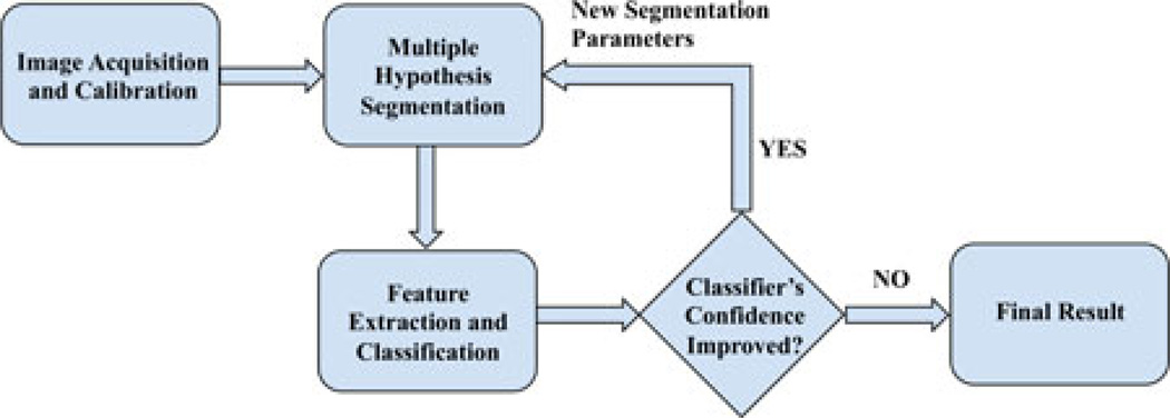
Fig. 2 is an overview of our approach, which we call the multiple hypotheses segmentation and classification (MHSC) system. Food images are acquired from a mobile device where a fiducial marker, currently a color checkerboard pattern, is placed in the scene to ensure color consistency due to changes in illumination and viewpoints. These images are sent to a server for the image analysis. A multiple hypotheses segmentation method (see Section II) is used to generate segmented regions, for which features are measured and classification is performed (see Sections III and IV). The classifier assigns to each segmented region a class label and a confidence score that indicates the “classifier’s confidence” that the label is correct. This information is evaluated based on a stability criteria (see Section V). If the stability condition is not satisfied, the segmentation step partitions the image again into a new set of segmented regions and the classification process is repeated. When the stability condition is satisfied, the classifier is no longer changing its class label decisions, the proposed system achieves the best possible class label for every pixel in the image.

Fig. 2.

Multiple hypotheses segmentation and classification.

Automatic identification of food items in an image is not an easy problem since foods can dramatically vary in appearance. Such variations may arise not only from changes in illumination and viewpoint but also from nonrigid deformations, and intraclass variability in shape, texture, color, and other visual properties. We fully understand that we will not be able to recognize every food. Some food items look very similar, e.g., margarine and butter. In other cases, the packaging or the way the food is served will present problems for automatic recognition. For example, if the food is in an opaque container then we will not be able to identify it. In some cases, if a food is not correctly identified, it may not make much difference with respect to the energy or nutrients consumed. For example, if our system identifies a “brownie” as “chocolate cake,” there is not a significant difference in the energy or nutrient content [1], [19]. Our goal is to provide a tool for better assessment of dietary intake to professional dietitians and researchers that is currently available using existing methods.

II. Multiple Hypotheses Segmentation

Given an unlabeled collection of images, our goal is to assign a class label to every pixel in the image corresponding to the object containing that pixel or declare it as “background” if the pixel does not belong to any of the specified classes. The output of our system is a labeled image with each pixel label indicating the class (object). We exploit the fact that segmentation methods are not stable as one perturbs their parameters, thus obtaining a variety of different segmentations. Many segmentation methods, such as normalized cut [20], use the number of segments as one of the input parameters of the segmentation method. Since, the exact number of segmented regions in an image is not known a priori, a particular choice of the number of regions results in either an under segmented or over segmented image. Furthermore, for a particular choice of the number of segmented regions, some objects may be under segmented, while others may be over segmented. That is, some of the segmented regions may contain pixels from more than one class while more than one segmented region may correspond to a single class. In order to obtain accurate segmentation of the image, we propose a joint iterative segmentation and classification system, where the classifier’s feedback (i.e., class label and confidence score) is used to obtain a final “stable” segmentation. We describe details of this process in Section V after explaining our segmentation method (see Section II), feature selection (see Section III) and choice of classifiers (see Section IV).

A. Salient Region Detection

Our segmentation method includes an initial step to identify regions of interest or salient regions. Unique to our application, we are interested in regions of an image containing food objects. The region of interest detection is useful for the task of assigning a correct label to each pixel by rejecting nonfood objects such as tablecloth, utensils, napkins, and thus reducing the number of pixels to be processed.

The first step is to remove the background pixels from our search space. We generate a foreground-background image by labeling the most frequently occurring color in the CIE L^*a^*b^* color space as the background pixel color. We identify strong edges present in each RGB channel of the image. In particular, we use the Canny operator to estimate the edges [21]. Edge pixels are linked together into lists of sequential edge points, one list for each edge contour. These edge lists are transferred back into a 2-D image array [22]. We combine background and edge images and remove undesired noise, such as holes, gaps, and bulges with morphological operations. We then label connected components in the binary image. Since food items are generally located in a plate, bowl, or glass that have distinctive shapes, our goal is to detect these objects. We first remove known nonfood objects such as the fiducial marker, currently a color checkerboard pattern, used as both a geometric and color reference [23]. To determine which components contain potential food items, we use the Canny edge filter [21] on each component and obtain the normalized edge histogram. The criteria for identifying components that contain food objects is experimentally determined to be the uniformity of the edge histogram. We compute the Euclidean distance between the normalized edge histogram of each salient region and a uniform distribution. Based on this criteria, a threshold is selected to determine a salient region.

B. Multiscale Segmentation

Multiscale segmentation approaches have achieved promising results. In [24], an algebraic multigrid technique is used to find an appropriate solution to the normalized cut measures, and a process of recursive coarsening is used to produce an irregular pyramid encoding of region-based grouping cues. Another method, proposed in [25] constructs multiscale edges with pairwise pixel affinity at multiple grids. Simultaneous segmentation through all graph levels is evaluated based on the average cuts criterion. We adopted the approach proposed in [26], where multiple scales of the image are processed in parallel without iteration to capture both coarse- and fine-level details. This approach uses the normalized cut [20] graph partitioning framework.

In the normalized cut, an image is modeled as a weighted, undirected graph. Each pixel is a node in the graph with an edge formed between every pair of pixels. The weight of an edge is a measure of the similarity between the two pixels, denoted as W_I (i, j). The image is partitioned into disjoint sets by removing the edges connecting the segments. The stable partitioning of the graph is the one that minimizes the weights of the edges that were removed (the cut). The method in [20] seeks to minimize the normalized cut, which is the ratio of the cut to sum of the weights of all of the edges in the set. Two simple yet effective local grouping cues are used to encode the pairwise pixel affinity graph. Since close-by pixels with similar intensity values are likely to belong to the same object, we can represent such affinity by

$$W_I(i,j)=\text{exp }[-(\frac{{\Vert I_i-I_j\Vert }_2^2}{{\sigma }_I^2}+\frac{{\Vert X_i-X_j\Vert }_2^2}{{\sigma }_X^2}\left)\right]$$ (1)

where I_i and X_i denote pixel intensity and location. Image edges are also strong indicator of the potential object boundary. The affinity between two pixels can be measured by the magnitude of image edges between them,

$$W_C(i,j)=\text{exp}\frac{-{\text{max}}_{x\in \text{line}(i,j)}{\Vert \text{Edge}(x)\Vert }^2}{{\sigma }_C^2}$$ (2)

where line(i, j) is the line joining pixels i and j, and Edge(x) is the edge strength at location x. We can combine these two grouping cues with tuning parameter α by

$$W_{\text{comb}}(i,j)=\sqrt{W_I(i,j)\times W_C(i,j)}+\alpha W_C(i,j).$$ (3)

The graph affinity W(i, j) exhibits very different characteristics at different ranges of spatial separation. Therefore, we can separate the graph links into different scales according to their underlying spatial separation,

$$W_{\mathit{\text{full}}}=W_1+W_2\approx W_1+{C_{1,2}}^T{W}_2{C}_{1,2}=W_{\text{reconstruction}}$$ (4)

where W_i contains affinity between pixels with certain spatial separation range and can be compressed using a recursive sub-sampling of the image pixels such as the use of interpolation matrix C_1,2 between two scales. This decomposition allows one to study behaviors of graph affinities at different spatial separations. The small number of short-range and long-range connections can have virtually the same effect as a large fully connected graph. This method is able to compress a large fully connected graph into a multiscale graph with O(N) total graph weights. The combined grouping cues are used with the CIE L^*a^*b^* color space. Selections of normalized cut parameters to generate the “stable” segmentation based on classifier’s feedback as shown in Fig. 2 are discussed in Section V.

C. Fast Rejection

Having a large pool of segments makes our overall methods more reliable; however, many segments are redundant and poor. These segments are results of selecting inappropriate clustering number in the segmentation step reflecting accidental image grouping. We deal with these problems using a fast rejection step. We first remove small segments (up to 500 pixels in area) in our implementation as these segments do not contain significant feature points to represent the object classes. We then assign background label to segments in each salient region detected previously. The number of segments that passes the fast rejection step is indicative of how rich or cluttered a salient region is.

III. Feature Description

An essential step in solving any object classification problem starts by determining the characteristics or features of the object that can be used to separate the object from other objects in the image. As mentioned earlier, feature spaces are formed by different types of features. Feature spaces formed by averaging features for an entire segmented region are known as global features, while feature spaces formed by features in local neighborhoods around points of interest or keypoints in the segmented region are known as local features. Both global and local features are used in our system.

A. Global Features

Color, texture, and shape are the three object representations most widely used for describing global characteristics of an object. In general, the segmentation step does not preserve the global shape information of an object. Also, most foods have large variations in shape based on eating conditions. Therefore, we use only color and texture descriptions as global features and not explicit shape information.

1. Global Color Features: Color is an important discriminative property of foods allowing one to distinguish, for example, between mustard and mayonnaise, and in some cases it is the only way to distinguish between liquids (e.g., orange juice and milk). Food shows large variation of color. Fresh food may contain different color chromaticities according to their ripeness and whether they are raw or cooked. Hence, there is no unique feature or color description that can be used to characterize food. In order to address many of the color effects found in foods, we considered three types of color features namely global color statistics, entropy color statistics, and predominant color statistics. First proposed for visual food description in [18].

   1. Global color statistics: consists of the first, and second moment statistics of the R, G, B, Cb, Cr, a^*, b^*, H, S, V color components corresponding to RGB, Y CbCr, L^*a^*b^*, and HSV color spaces, respectively. One feature vector is obtained for the entire image segment; containing the two moments for each color component.
   2. Entropy color statistics: this feature characterizes the distinctiveness and repeatability of color information for each color space component using entropy [27]. The feature vector is formed by estimating the first- and second-moment statistics of the entropy in RGB space components for the entire segmented region.
   3. Predominant color statistics: our third color descriptor aims at capturing the distribution of the salient colors in the object by selecting the P most representative colors (in RGB space) for a segment. The feature vector for this color descriptor is defined as

      $$F=\{(c_1,p_1,{\upsilon }_1),\dots ,(c_P,p_P,{\upsilon }_P)\}$$ (5)

      where c_i represents the 3-D color vector from the RGB cube, p_i is the percentage of color in the total object, and υ_i is the color variance inside the region described by the predominant color. The total dimension of the feature vector is (7 × P). A similar color descriptor is used in the MPEG-7 standard, known as the dominant color descriptor [28].
2. Global Texture Features: For many object categories, texture is a very descriptive feature. In our system, we used three texture descriptors for food classification [29]: Gradient Orientation Spatial-Dependence Matrix (GOSDM), Entropy-based categorization and Fractal Dimension estimation (EFD), and a Gabor-based image decomposition and Fractal Dimension estimation (GFD).

   1. Gradient Orientation Spatial-Dependence Matrix: Describes the spatial relationship between gradient orientations by means of the occurrence of pairs of gradient orientation values at offsets d (length and orientation). For each magnitude of d (2⁰, 2², 2⁴, …), we determined four GOSDMs based on the following angular directions: 0°, 45°, 90°, 135°. As in the case of GLCM features, several statistics were used to compress the amount of information of each GOSDM [30]. These are Correlation (COR), Angular Second Moment (ASM), Entropy (ENT), Contrast (CON), and Homogeneity (HOM).
      Once these measures are determined, the final step is to create the feature vector for the entire texture region. For an H × V texture region it is defined as [7], [29]:

      $$\mathbf{f}=[f_{d_1}\hspace{1em}{f}_{d_4}\hspace{1em}{f}_{d_{16}}\dots f_{d_{\text{min}(\mathrm{H}/2,\mathrm{V}/2)}}]$$ (6)

      where the vector f_di is defined as f_di = [COR_0°ASM_0°ENT_0° CON_0°HOM_0°COR_45°ASM_45°ENT_45° CON_45° HOM_45° COR_90°ASM_90°ENT_90°CON_90°HOM_90°COR_135°ASM_135° ENT_135°CON_135°HOM_135°]_i.
   2. Entropy categorization and fractal dimension estimation: Our second texture descriptor is based on multifractal analysis [31], [32]. We examined a multifractal analysis of textures using entropy [7], [29]. Given a pixel x and a local neighborhood M_p, we first estimate its entropy H_x. Once the entropy is estimated for all the pixels in the texture image, we cluster regions where the entropy function exhibits similar values. For a given entropy value υ, ϒ_υ represents the set of pixels {x : x ∈ H × V and H_x ∈ (υ, υ + δ)}, for some arbitrary δ. Once this pixel categorization is completed, we estimate FD_ϒυ, the fractal dimension (FD) for each ϒ_υ by following the approach presented in [33]. The final texture feature is formed by fusing all the FD_ϒυ into one single-feature vector.
   3. Gabor-based image decomposition and fractal dimension estimation (GFD): Our third texture descriptor is also based on multifractal theory [31], [32], and it uses Gabor filterbanks [34]. For each scale (m = 0, 1, …, S − 1) and orientation (n = 0, 1, …, K − 1), we estimate the FD of the image filter response (I_{gm, n}), FD_{Igm, n}. The final descriptor becomes f = [FD_{Ig 1, 1} FD_{Ig 1, 2}⋯FD_{Ig S ,K}].

B. Local Features

Low-level features based on multiscale or scale-space representation were also examined. The main difference with global features is the size of the region used to estimate the features. Local features are estimated around points located in regions of the image. These locations are often called points of interest or keypoints. They are described by the local appearance of the group of neighboring pixels surrounding the point location.

We have used a series of local feature spaces including SIFT [35] and SURF [36] descriptors. We also used steerable filters [37] which are a bank of randomly oriented filters. In this case, we used 2-D circularly symmetric Gaussian functions and obtain the first- and second-moment statistics of the response of the filtered local image neighborhood with the steerable filterbank. We used five orientations and up to fifth-order Gaussian derivative. Finally, we also used SIFT descriptors on the R,G,B color components separately since we were also interested on capturing local color information (Red-SIFT, Green-SIFT, and Blue-SIFT).

Overall for each segmented object, we constructed 12 feature spaces (feature channels): three global color feature channels (Global color statistics, Entropy color statistics, and Predominant color statistics), three global texture channels (GOSDM, EFD, and GFD), and finally six local feature channels (SIFT descriptor, Red-SIFT descriptor, Green-SIFT descriptor, Blue-SIFT descriptor, SURF, and Steerable filters). Table I in Section VI shows all the features as well the feature space dimension.

TABLE I.

Mean Classification Rate for All Classes for Each Type of Feature Channel Using the KNN and SVM Classifiers

Feature Channel	Type	Dimension	Mean classif. rate KNN	Mean classif. rate SVM
Color Stats.	Global Color	20/segment	0.68	0.62
Entropy Color Stats.	Global Color	6/segment	0.20	0.35
Pred. Color Stats.	Global Color	28/segment	0.42	0.60
EFD	Global Texture	120/segment	0.39	0.47
GFD	Global Texture	120/segment	0.23	0.27
GOSDM	Global Texture	60/segment	0.32	0.32
SIFT	Local	128/keypoint	0.44	0.48
Red-SIFT	Local	128/keypoint	0.45	0.48
Green-SIFT	Local	128/keypoint	0.44	0.49
Blue-SIFT	Local	128/keypoint	0.47	0.47
SURE	Local	128/keypoint	0.43	0.45
Steerable Filters	Local	50/keypoint	0.39	0.43

IV. Classification

In Section III, we described the features we are using to form feature vectors f. Given an unlabeled collection of images, our goal is to assign a class label to every pixel in the image corresponding to the object containing that pixel or declare it as “background” if the pixel does not belong to any of the specified classes. The output of our system is a labeled image with each pixel label indicating the class (object).

In this section, we describe our system for classifying objects, from segmented input images, given training segmented regions and their feature vectors (supervised learning) using several machine-learning strategies. Note that we distinguish between training segmented regions and testing segmented regions. Each class/label (food class) is composed of many training objects S_t, and their associated feature vectors, f_t. Testing data refers to segmented regions S_q obtained from the input image I_q that the system has yet to classify after forming testing feature vectors f_q at the feature extraction stage.

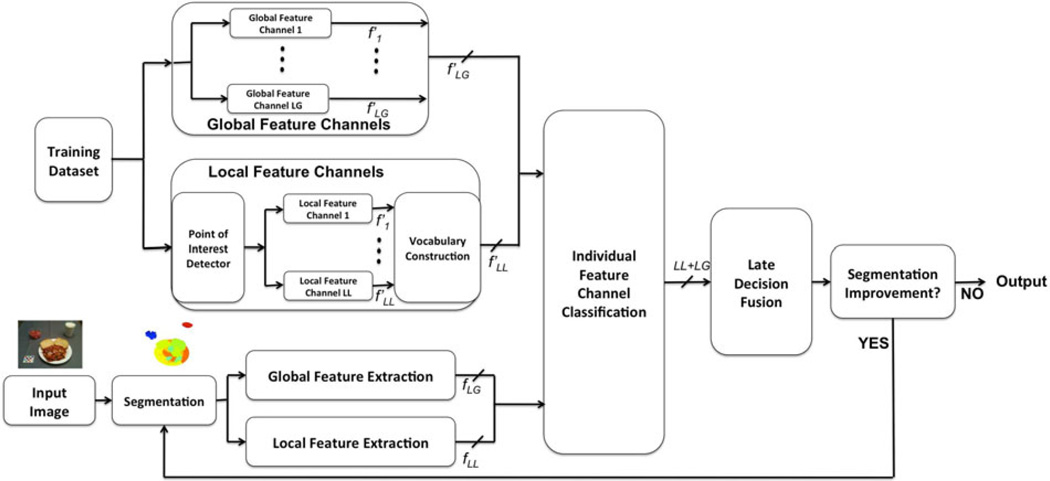
We have followed the works presented in [38] and [39] where authors have shown how decision-level fusion outperforms feature-level fusion for very different datasets, and in [40] where authors have shown how combination of individual classifiers improves significantly the contribution of individual classifiers. We propose a multichannel feature classification system, where each feature channel (feature type) is individually classified. We have 12 feature channels that consists of three global color feature channels: Global color statistics, Entropy color statistics, and Predominant color statistics, three global texture feature channels, namely GOSDM, EFD, and GFD, and finally, six local feature channels SIFT descriptor, Red-SIFT descriptor, Green-SIFT descriptor, Blue-SIFT descriptor, SURF, and Steerable filters. As a result of this process, 12 class decisions are obtained for each segmentation region. The next step is to obtain the final classification based on the 12 individual classifier decisions by fusing the results of the 12 classifiers. We call this late decision fusion. Fig. 3 shows the components of our classification system.

Fig. 3.

Classification System. (LG is the number of global feature channels and LL is the number of local feature channels. f′(․) corresponds to the training feature set, and f (․) corresponds to features of the image.)

A. Individual Classification

We have examined two classifiers, KNN and SVM, to classify the feature channels. The KNN classifier consists of assigning a class label based on data proximity in a n-dimensional feature space. It estimates a distance measure (e.g., Euclidean distance), in the feature channel l between the testing feature vector $f_d^{(l)}$, and each of the training feature vectors $f_t^{(l)}$, and then, selects the class with at least K of the training feature vectors closest to the testing feature vector [41]. KNN bases its decision on data locality (only the K closest training feature vectors are considered). The goal of an SVM is to produce a classification model by constructing an N-dimensional hyperplane that optimally separates the training data (feature vectors) into classes or feature space partitions [42]. We used the publicly available SVM toolbox [43]. Before the supervised classification, KNN or SVM, there is a step known as vocabulary construction and signature formation. This is known as bag of features (BoF) [44], [45]. Local features are used to build visual vocabularies that are formed by using an unsupervised learning strategy such as clustering. Each cluster of local features represents a visual word. We use a hierarchical version of k-means, where each local feature space is recursively divided into clusters [46]. For each segmented region of the test image, local features are extracted and propagated down the tree. A signature is formed by estimating the distribution of the visual words in the segmented region (e.g., how many times each visual word in the vocabulary occurs in the segmented region S_q). This distribution is known as the signature of the object [45]. For each local feature channel one signature is obtained. We used the signature as input to the individual local feature channel classifiers (i.e., KNN or SVM). For the experiments presented in Table I, the dimensionality of our signatures is 1110 (the size of the visual vocabulary).

B. Combination of Local and Global Features

As a result of the individual multichannel classification, we obtain 12 class labels for each segmented region for an input image. A final decision needs to be obtained from these decisions [40]. We fuse the outputs of the individual feature channel classifiers for a final class decision [38]. Hence, we are individually classifying each feature type and combining classifier decisions along with distance-based confidence scores given the best β candidate classes for each feature channel. By candidate classes, we mean the most likely class labels that a classifier selects and ranks given an input segmented region S_q.

The confidence score indicates the likelihood that the identified class label is correct. It is estimated using only the feature vectors of the training samples from each class that contribute to the classification, e.g., in the KNN case only the K closest samples of an identified class are used to estimate the classifier’s confidence. The confidence score ψ(S_q, λ), of the KNN classifier for assigning segmented region S_q of an input image I_q to class λ in feature channel l is defined as

$${\psi }_l{(S_q,\lambda )}^{(k-NN)}=\frac{1}{k}\sum _{i=1}^k\frac{\text{exp}(-d(f_{S_q},f_{S_{\lambda }^i}))}{(d_{1-NN}+\epsilon )},\text{for each }\lambda \in \mathrm{\Lambda }$$ (7)

where $d(f_{S_q},f_{S_{\lambda }^i})$ represents the distance between the normalized feature vector of the input segmented region S_q, f_Sq, and the normalized feature vector of the ith nearest neighbor training sample belonging to class λ, $f_{S_{\lambda }^i}·d_{1-\mathrm{N}\mathrm{N}}$ represents the distance between the normalized feature vector of the input segmented region S_q, and the nearest neighbor (1−NN), we add ε to the denominator to avoid division by zero; this was set to machine epsilon (i.e., the relative error due to rounding in floating point arithmetic). Λ is the collection of class labels.

Similarly, when SVM is used, then the classifier’s confidence score is

$${\psi }_l{(S_q,\lambda )}^{(\mathrm{S}\mathrm{V}\mathrm{M})}=\frac{\text{exp}(-d(f_{S_q},f_{S_{\lambda }^i}^{(\text{ave})}))}{(d_{1-NN}+\epsilon )},\text{for each }\lambda \in \mathrm{\Lambda }$$ (8)

where $d(f_{S_q},f_{S_{\lambda }^i}^{(\text{ave})})$ represents the distance between the normalized feature vector of the input segmented region S_q, f_Sq, and the normalized average feature vector for class λ, $f_{S_{\lambda }^i}^{(\text{ave})}$. For the local features, the average class feature vector $f_{S_{\lambda }^i}^{(\text{ave})}$ is a feature vector containing the frequency that each visual word is observed in class λ on average. Average feature vectors can be thought of as feature prototypes to represent each class. They have been shown to increase classification accuracies [47], [48].

Two strategies are considered for the final fusion decision given as follows:

1. Maximum confidence score: This consists of choosing the class label such that the confidence score from all the feature channel classifiers is the largest. That is, for each segment S_q select the class such that it satisfies $\hat{\lambda }(S_q)={\text{argmax}}_{{\lambda }^{*}\in |\mathrm{\Lambda }|}({\sum }_{l=1}^L{\sum }_{b=1}^{\beta }{\psi }_l^b(S_q,{\lambda }_l^b))$, with L being the number of feature channels.

2. Majority vote: Here the majority vote on the set ${\lambda }_1^{b=1},\dots ,{\lambda }_L^{b=1}$ is used. In the case of the same number of votes, the tie-breaker is the output of the individual classifier that achieves higher classification rate (most salient feature). Majority rule can be seen as a variation of the maximum confidence score for the case that all KNN are equal distance in the feature space from the input segment.

As a result of using multiple feature channels and combining them into one final class decision, we obtain a set of candidate classes for each segmented region in the input image Λ_m,C (S_q), which correspond to the top C most likely classes for a given input segmented region S_q and a segmentation hypothesis, m. A segmentation hypothesis is obtained by varying the number of segmented regions for each input image. Each final candidate class λ̂_m,c = λ̂(S_q) has a final confidence score associated with it defined as

$$\mathrm{\Psi }(S_q,{\hat{\lambda }}_{m,c})=\frac{1}{L}\sum _{i=1}^L{\psi }_l(S_q,{\hat{\lambda }}_{m,c}),$$ (9)

where L = 12 is the total number of feature channels, and ψ_l (․, ․) represents the confidence score per feature channel, and Ψ(․, ․) the final confidence score of the classifier to label segment S_q with label λ̂_m,c.

V. Stable Segmentation via Iteration

As we described earlier in Fig. 2, results from the classifier are used as feedback to select the “stable” parameters of the normalized cut segmentation method used in each salient region. This iterative approach generates the final “stable” segmentation based on the improved classifier’s confidence. Through iteration, each segmentation hypothesis generated by the normalized cut vary in the number of segments and class labels; thus, there are errors in different regions of the image. Our challenge is to determine which parts of the hypotheses are likely to be correct and combine the hypotheses to accurately locate the objects and determine their class labels. Since the “correct” number of segments Q that yield a “stable” segmentation is unknown a priori, we explore all possible parameter settings.

We propose an iterative stability framework for joint segmentation and classification. To produce multiple segmentations, we vary the number of segmented regions Q(the “segmentation parameter” in the normalized cut method) in two ways depending on the size of the salient region. Q = 3 is used as the initial number of segmentations for salient regions less than 250-pixels in length or breadth of a bounding box, and Q = 7 for larger salient regions. Let S_q (i, j)^m denote the segmented region containing pixel I_q (i, j), for the mth iteration of the segmentation and classification steps. Λ_m,C (S_q (i, j)) denotes the set of C candidate class labels for segmented region S_q (i, j) for the mth iteration. The set of C candidate class labels for pixel I_q (i, j), after M iterations is denoted by ${\mathrm{\Lambda }}_{M,C}^{\star }(I_q(i,j))$. The candidate class with highest confidence score ${\lambda }_{M,c}^{\star }(I_q(i,j))$ is estimated based on the cumulative confidence scores Ψ^M (I_q (i, j), λ) defined as ${\lambda }_{M,c}^{\star }(I_q(i,j))=\underset{\hat{\lambda }\notin {\mathrm{\Lambda }}_{M,C-1}^{\star }}{\underbrace{\text{argmax}}}{\mathrm{\Psi }}^M(I_q(i,j),\hat{\lambda })$ where

$${\mathrm{\Psi }}^M(I_q(i,j),\hat{\lambda })=\frac{{\sum }_{m=1}^M{\sum }_{{\lambda }_i\in {\mathrm{\Lambda }}_{m,C}{(S_q(i,j))}^1{({\lambda }_i=\hat{\lambda })}^{\mathrm{\Psi }(S_q{(i,j)}^m,\hat{\lambda })}}}{{\sum }_{{\lambda }_i\in {\mathrm{\Lambda }}_{m,C}{(S_q(i,j))}^1({\lambda }_i=\hat{\lambda })}}.$$ (10)

In each iteration, every pixel is assigned the class label that has the highest cumulative confidence scores up to the current iteration. Note that λ̂_m,c is a candidate class label generated from an input segmentation parameter for the current mth iteration. ${\lambda }_{m,c}^{\star }$ is the best candidate class label based on the cumulative confidence scores after m iterations.

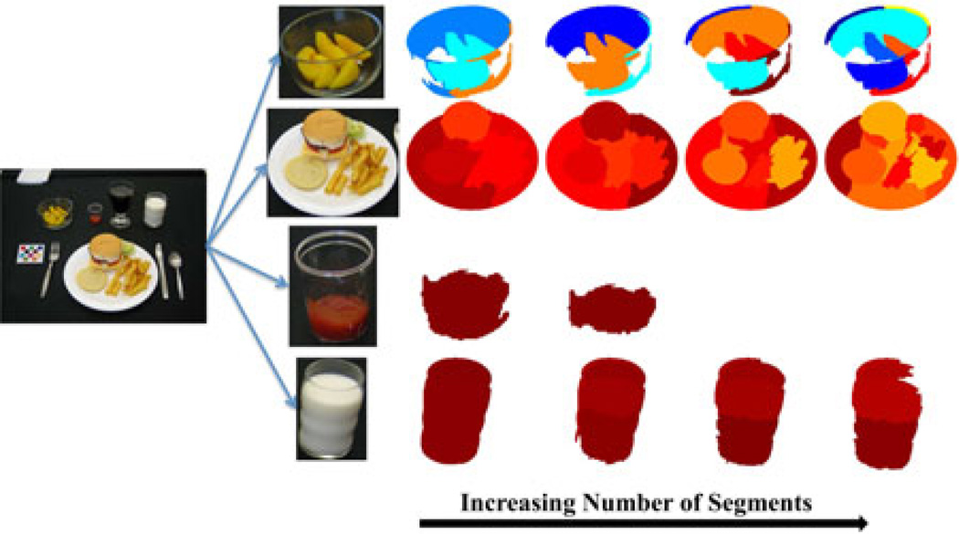
The pixel label becomes stable when the cumulative confidence scores does not show improvement. The iteration process stops when the percentage of pixel labels being updated is less than 5% for each segment. This means the image region has been segmented properly (“stable” segmentation) based on the stability of the classifier’s confidence scores. In general, we achieve the “stable” results after four iterations. Fig. 4 shows multiple segmentations generated from each iteration of the joint segmentation and classification approach for every salient region detected from the input image shown in Fig. 1. The number of segmented regions Q is increased for each iteration. Some regions may require fewer iterations to reach the “stable” segmentation than others. For example, region containing ketchup requires only two iterations, while other salient regions require four iterations for this meal image.

Fig. 4.

Multiple segmentations obtained from the salient regions.

The output is a labeled map with each pixel assigned to the best class label. The iterative stability measure depends on the classifier’s confidence of the assigned label for each segment being correct; thus, the performance of the classification plays an important role. The correct class label of the segment requires accurate detection of the object boundary so that features extracted from the segment can be closely matched to features of objects in the training images. Therefore, a high confidence score of the classifier not only implies strong visual similarity between the identified object and its training data, but also accurate boundary detection from the segmentation. It is unlikely that the classifier will have 100% accuracy even with perfect segmentation because some foods are inherently difficult to classify due to their similarity in the feature space. Examples of these are illustrated in Section VI.

VI. Experimental Results

The proposed system was tested on a collection of food images acquired by participants during nutritional studies conducted by the Department of Nutrition Science at Purdue University. We also have ground-truth information, done manually, for the images including the segmentation regions for each food item and the corresponding class label. This will be used for system performance evaluation. In our dietary assessment system, the image segmentation and classification part are performed on the server. In a typical scenario, the server takes less than 30 s to analyze a 3-MP image.

A. Quantitative Evaluation of Segmentation Performance

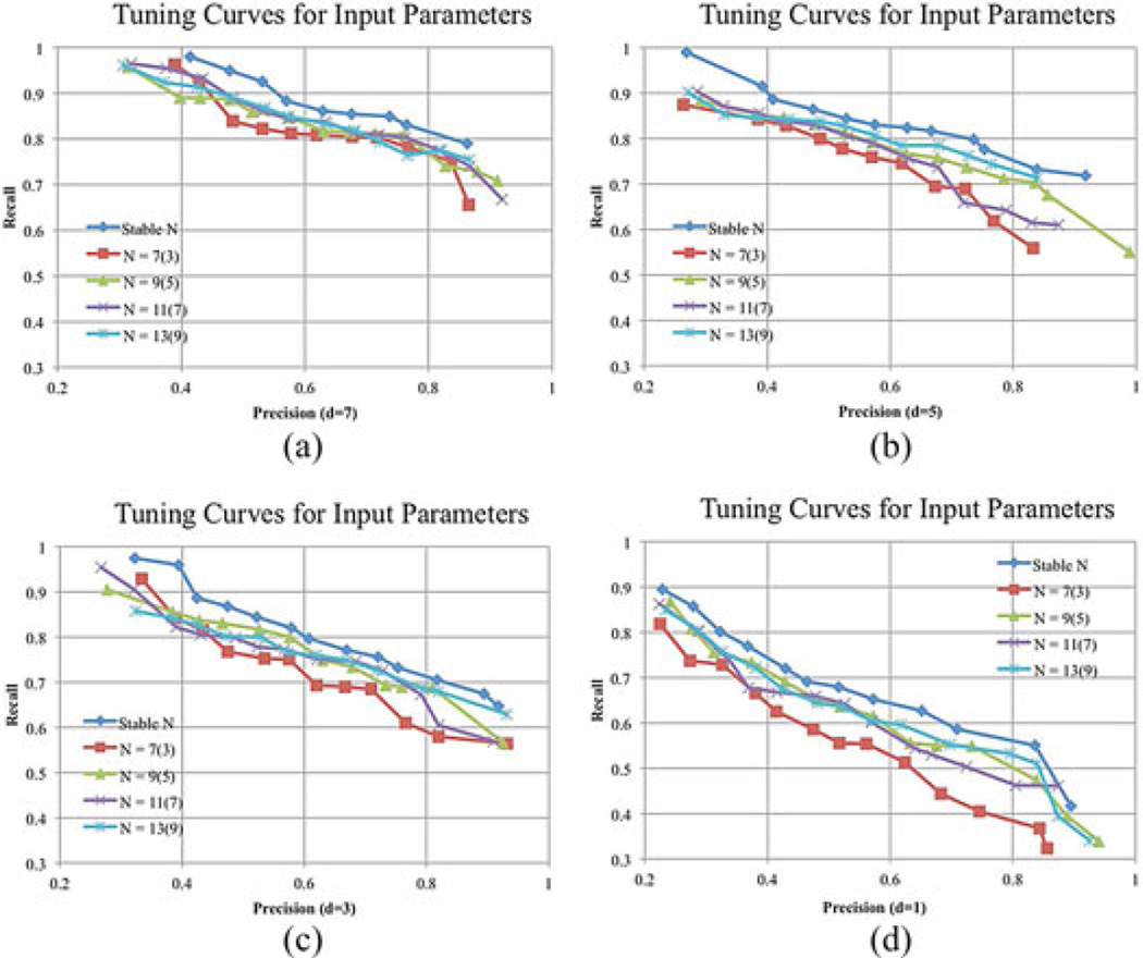
We are interested in evaluating our proposed methods based on quantitative measures of segmentation quality. In particular, the disparity between an actually segmented image and the ideal segmented image (ground-truth) can be used to assess performance. We used the method proposed by Estrada et al. [49] to generate precision/recall scores for a range of input parameters (number of segments between 3 and 13) of the normalized cut method, the stable parameter, as well as manual segmentation. Precision is defined as the proportion of boundary pixels in the automatic segmentation that correspond to boundary pixels in the ground truth, while recall is defined as the proportion of boundary pixels in the ground truth that were successfully detected by the automatic segmentation.

Given two segmentations S₁ and S₂, a suitable match for each boundary pixel in S₁ was found by examining its neighborhood within a radius of d for boundary pixels in S₂. A pixel b_i in S₁ was matched to a pixel b_x in S₂ when the following conditions were satisfied.

1. No other boundary pixel b_j in S₁ exists between b_i and b_x.

2. The closest boundary pixel in S₁ for pixel b_x is in the specified direction of b_i. If b_x has several closest neighbors, at least one must point in the specified direction of b_i. In practical implementation, this means the directions from b_x to b_i, and from b_x to one of its closest neighbors must be within 25° of each other.

In the case where more than one pixel in S₂ satisfies the listed conditions for pixel b_i, we select the nearest one.

To obtain a meaningful benchmark, for each combination of parameters, we tested the methods on a set of 130 food images. The scores for a particular combination of input parameters is the median of the precision and recall scores obtained for the individual image. The median precision and recall scores computed for different combinations of input parameters yield tuning curves characterizing the performance of the methods.

Since the normalized cut and our multiple hypotheses segmentation approach take only one input parameter, which is the desired number of segments, we tested these methods for a number of output segmented regions within a range of input parameters that yield reasonable segmentations appropriate for our dataset. For the normalized cut method (no classifier feedback), the range of input parameter is [3,13]. Our segmentation method automatically selects the stable input parameter from the classifier feedback.

We choose for comparison the tuning curves resulting from various precision and recall scores. From these curves, the appropriate parameters can be selected that will yield a target value of either precision or recall for a given method. More importantly, they provide a direct way of comparing the quality of the segmentation produced by different methods across a wide range of input parameters. We can tell from these tuning curves if a method performs consistently better than others across its particular range of parameters, and then rank methods by performance for particular values of precision or recall.

Fig. 5 shows quantitative evidence that our proposed segmentation method including the class label information and the classifier’s confidence score outperforms the normalized cut (no classifier feedback) across the range of tested input parameters. Comparing the four sets of curves, the scores for all tuning curves fall sharply as d decreases. This is consistent with the observation made by Martin et al. [50] and supports the use of a smaller matching radius during evaluation.

Fig. 5.

Tuning curves for a normalized cut (no classifier feedback) and our MHSC segmentation (with classifier feedback) for (a) d = 7, (b) d = 5, (c) d = 3, and (d) d = 1. The stable input parameter is automatically chosen based on the segmentation method.

B. Feature and Classification Evaluation

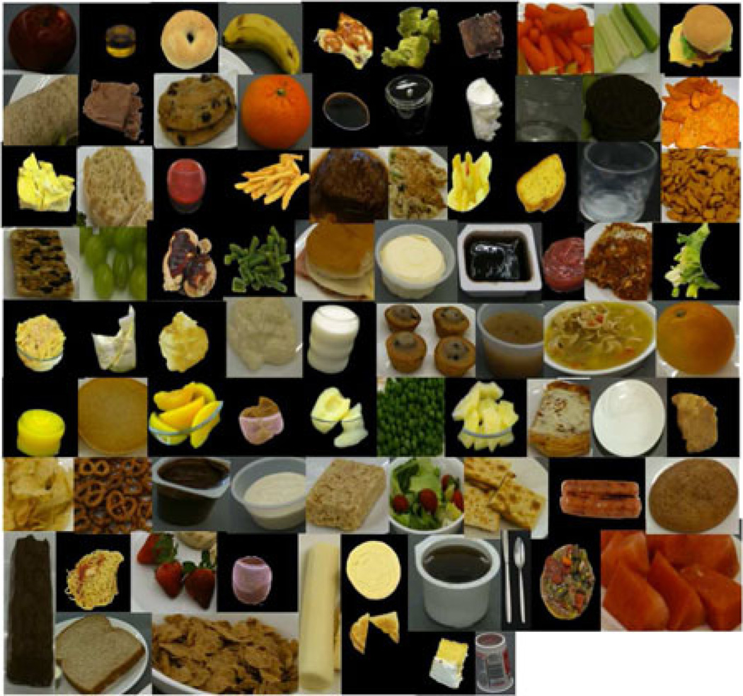
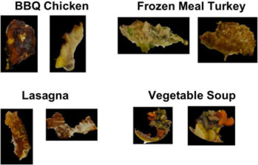
In the previous section, we presented results of combining segmentation and classification for quantitative measures of segmentation quality. In this section, we show evaluation results of our proposed classification system performance in terms of correct classification accuracy given a set of segmented regions. The goal was to measure the efficiency of the features for food characterization. For this set of experiments, we considered 83 classes (79 food classes, and utensils, glasses, plates, and plastic cups). Each class contained many segmented regions or samples obtained from the segmentation of meal images. The number of samples in each class varies, with 20 being the minimum number of samples for some classes and 50 being the maximum, and an average of 30 per class. Fig. 6 shows manually segmented examples of each food item. Fig. 7 shows examples of the automatic segmentation regions used in our system.

Fig. 6.

Examples of 83 food classes used in our experiments.

Fig. 7.

Examples of segmented regions: BBQ chicken, frozen meal turkey, lasagna, and vegetable soup.

First, we compared the information captured by each of the 12 feature channels. Table I shows mean correct object classification rates for each feature channel for both classifiers: KNN and SVM. In the experiments 60% of the data were used for training and 40% for testing. Experiments were repeated 10 times with random selection of training and testing data. Note that in the SVM case, global color statistics, entropy color statistics, EFD, SIFT, Red-SIFT, Green-SIFT, Blue-SIFT, and Steerable filters, GOSDMs were classified using RBF kernels, and for predominant color statistics, GFD and SURF descriptor we used quadratic kernels. In all cases, we set gamma (SVM parameter) as being the inverse of the average number of feature vectors (number of classes times average number of instances per class): 0.001 < γ < 0.0001. We set C as the number of classes, C = 83. Only when both γ and C were low (<0.01) the SVM performance was substantially degraded. These parameters were determined after cross-validation experiments. As shown, global color statistics feature outperformed the other color features in all tests considered. Among the texture features EFD performed better than the other two types of features: GFD and GOSDM. Also, local features and the BoF approach have proven to be very efficient. These results show the importance of color information to globally describe food segments. Finally, local features such as SIFT achieved high performance, but so did Red-SIFT, Green-SIFT, and Blue-SIFT which indicates that color information may also be relevant to describe objects locally. From these results, we also observed that, in general, for local features SVM performs better than KNN.

After the individual channel classification, the next step in our classification system is to obtain the final class decision by combining individual decisions. The experiment consisted of comparing our two decision fusion methods as a function of the number of candidate classes (1 and 8) on each feature channel. Candidate classes refer to the most likely class labels (top ranked) for each feature channel that a classifier selects given an input segmented region. By using more than one candidate for each feature channel, the probability that the true (correct) label be among the class candidates increases. Table II shows the performance of both decision fusion approaches. For reference, we have compared our decision-based classifiers with two other types of classifiers: SVM feature concatenation and Fisher vectors encoding on SIFT features [51]. SVM feature concatenation refers to concatenate feature vectors into one vector. In our case the best performing feature channel of each type (Table I): color statistics for color, EFD for texture, and SIFT for local features were used. SVM kernels, of the three feature channels, were linearly combined into one single kernel for classification. Fisher vector encoding has been evaluated using the publicly available VLFEAT library [52].

TABLE II.

Average Classification Rate for Each Decision Fusion Approach Majority Vote Rule and Maximum Confidence Score for Both KNN and SVM Classifiers for Multiple Candidates (1, and 8)

Decision Fusion (Classifier)	1 Candidate	8 Candidates
Majority vote rule (KNN)	0.70	0.74
Maximum confidence score (KNN)	<0.1	0.75
Majority vote rule (SVM)	0.57	0.72
Maximum confidence score (SVM)	0.33	0.70
SVM concat.	0.52
SIFT FV	0.61

And comparison with SVM feature concatenation (SVM concat.) and Fisher vector encoding with SIFT (SIFT FV).

The best performance was achieved combining decisions obtained using KNN for large number of candidates. We observed, that decision fusion strategies require orthogonal feature spaces, i.e., feature channels that complement each other. From the results, data locality-based classifiers such as KNN have more consistent class decision when considering multiple candidates, even for very independent feature spaces when compared to efficient classifiers such as SVM. Performing late decision fusion shown an improvement compared to the performance of individual classifiers. These results are aligned with earlier work presented in [38]–[40], and [53], where similar late decision fusion algorithms outperformed individual classifiers. Comparing both decision rules, we observed that maximum confidence score has a great dependance upon the training data since it bases its efficiency on the visual appearance compactness of a class to assign scores. If unstable segmented regions within each class have large variation in appearance, majority rule proved to be a better solution.

We also observed that simple decision rules like majority vote rule can be a better choice for feature fusion as opposed to concatenate the best performing individual features into one single vector and apply SVM. Late decision fusion rules and combination of different type of features can also be competitive in terms of classification accuracy compared to other state-of-the-art algorithms like Fisher vector encoding using SIFT features that have proven its efficiency in image classification tasks [54].

We were also interested in determining the contribution of each feature channel into the final food classification decision to identify which features are more salient for food classification. We measured it as the ratio between the number of total correct classification foods for a particular feature channel and the number of total correct classification foods of the overall system. Global color statistics contributed 0.760 to the final decision, entropy color statistics achieved 0.485, predominant color statistics 0.650, EFD 0.648, GFD 0.442, GOSDM 0.567, SIFT 0.794, Red-SIFT 0.835, Green-SIFT 0.830, Blue-SIFT 0.831, SURF 0.751, Steerable 0.720 agreement with the final decision. From these results, we observed that SIFT-based features had a large contribution on the overall system; however, simple color statistics can also provide salient food descriptions. In terms of type of features, on average local features contributed the most with an overall contribution rate of 0.793 versus color and texture features with 0.631 and 0.552, respectively. In case only complex foods were considered (foods with many ingredients such as cheeseburger, soups, sandwiches), local features achieved even a higher contribution rate, 0.882, which indicates how descriptive these type of features are for complex objects in contrast with global color and texture features that describe more uniform characteristics.

Our evaluations combine errors from both segmentation and classification. If an image is perfectly segmented, i.e., it completely agrees with the ground truth, the error in classification contributes to pixels being incorrectly labeled. If a region of the image is poorly segmented, it may not represent the visual characteristics of associated food class, therefore resulting in wrong class labels for pixels belong to that region. As it has been mentioned before some foods are inherently difficult to classify due their similarity in the feature space; others are difficult to segment due to faint boundary edges that camouflage the food item; as well as the nonhomogeneous nature of certain foods. In order to measure the joint performance of segmentation and classification, we looked at the improvement obtained as a result of applying our iterative approach versus a one-pass segmentation and classification strategy in terms of the per pixel accuracy. Per pixel accuracy is obtained by comparing the class label assigned to each pixel to ground-truth information. On average, we observed an increase of 22% classification accuracy in the final iteration with respect to the initial (one-pass) iteration.

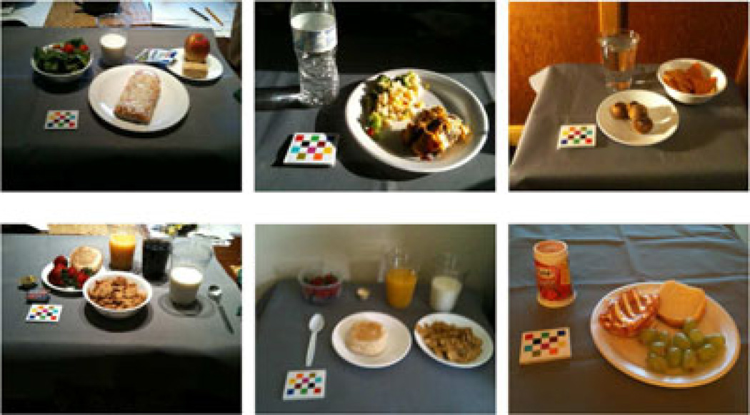
Another challenge that we face in our system is the large variation of illumination conditions observed in images acquired by users. Fig. 8 show several examples of images acquired by users with very different illumination conditions. In order to deal with large number of food classes and different illumination conditions our dietary assessment system [2] has the ability to output a set of class labels (food suggestions) for each object in the image. This set consists of the top four ranked food classes. This information is used by the user to select the true food class. By measuring the performance of the system with respect to whether the true food class is within the four suggestions, we can increase the food classification rate by 30%, and thus achieve very high classification accuracies for large number of foods and illumination conditions [7]. The user’s feedback also allows the system to learn the user eating pattern. Currently, we are investigating the integration of a user’s eating pattern into training the classifier to further increase the efficiency of our classification system, as well as other contextual information like eating locations, times and dates.

Fig. 8.

Examples of images acquired by users exhibiting large illumination variations.

VII. Conclusion

We have described a segmentation and classification system based on generating multiple segmentation hypotheses by selecting segmentations using confidence scores assigned to each segment. Evaluation of the proposed MHSC method shows that our approach outperforms the normalized cut method. This also agrees well with the visually perceived quality of the corresponding segmentations. We have also investigated global and local features in order to provide a more complete description of objects. We have shown that by individually classifying each feature channel and doing late decision fusion based on the individual classifier’s decisions and their confidence scores, we can increase the classification rates for each individual classifier. Based on our evaluations, we have shown improved accuracy of segmenting food images using our segmentation approach compared to normalized cut without classifier feedback when there is no prior information about the scene. This translates into an overall improved classification accuracy. Overall we have shown that our methods can be integrated into an image-based dietary assessment system.

Biographies

Fengqing Zhu (S’05–M’12) received the B.S., M.S. and Ph.D. degrees in electrical and computer engineering from Purdue University, West Lafayette, IN, USA, in 2004, 2006, and 2011.

During the summer of 2007, she was a Student Intern at the Sharp Laboratories of America, Camas, WA, USA. She is currently a Staff Researcher at Huawei Technologies (USA), Santa Clara, CA. Her research interests include video compression, image/video processing and analysis, computer vision, and computational photography.

Marc Bosch (S’05–M’12) received a degree in Telecommunications engineering from the Technical University of Catalonia (UPC), Barcelona, Spain, in 2007, and the M.S. and Ph.D. degrees in electrical and computer engineering from Purdue University, West Lafayette, IN, USA, in 2009 and 2012, respectively. In 2012, he joined Texas Instruments as a Computer Vision/Computational Photography Engineer. He is currently a Senior Video Engineer at Qualcomm, Inc, San Diego, CA, USA. His research interest include image/video processing, computer vision, machine learning, and computational photography.

Dr. Bosch received the Archimedes Award for the best undergraduate engineering thesis in Spain from the Science and Education Ministry of Spain in 2007. He received the Meritorious New Investigator Award at the 2010 mHealth Summit.

Nitin Khanna (S’07–M’10) received the B. Tech. degree in electrical engineering from the Indian Institute of Technology, Delhi, India, in 2005, and the Ph.D. degree in electrical and computer engineering from Purdue University, West Lafayette, IN, USA, in 2009.

From 2009–2012, he was working as a Post-Doctoral Research Associate in the Video and Image Processing Laboratory, School of Electrical and Computer Engineering, Purdue University. Since 2012, he has been an Associate Professor in the Department of Electronics and Communication Engineering, Graphic Era University, Dehradun, Uttarakhand, India.

Carol J. Boushey received the B.Sc. degree from the University of Washington, Seattle, WA, USA, and the Masters of Public Health from the University of Hawaii at Manoa, Honolulu, HI, USA, and the Ph.D. degree from the University of Washington through the interdisciplinary nutrition program and the epidemiology program. She is an Associate Researcher at the University of Hawaii Cancer Center and Adjunct Professor at Purdue University, West Lafayette, IN, USA. She has directed two multisite randomized school trials, No Bones About It! and Eat Move Learn; and the statewide Safe Food for the Hungry program in Indiana. Her research interests include dietary assessment methods, adolescent dietary behaviors, school-based interventions, food insecurity, and applications of quantitative methods.

Dr. Boushey serves on the Board of Editors of the Journal of The American Dietetic Association. She is the Coeditor for the second edition of Nutrition in the Treatment and Prevention of Disease (spring of 2008, Elsevier). Her published research has appeared in book chapters and journals, such as Pediatrics, the Journal of Nutrition, and JAMA. She has presented on numerous occasions at regional, statewide, national, and international meetings. She is currently a Registered Dietitian with the Commission on Dietetic Registration.

Edward J. Delp (S’70–M’79–SM’86–F’97) was born in Cincinnati, OH, USA. He received the B.S.E.E. (cum laude) and the M.S. degrees from the University of Cincinnati and the Ph.D. degree from Purdue University, West Lafayette, IN, USA.

In May 2002, he received an Honorary Doctor of Technology from the Tampere University of Technology, Tampere, Finland. From 1980 to 1984, he was with the Department of Electrical and Computer Engineering, The University of Michigan, Ann Arbor, MI, USA. Since August 1984, he has been with the School of Electrical and Computer Engineering and the School of Biomedical Engineering, Purdue University. He is currently The Charles William Harrison Distinguished Professor of Electrical and Computer Engineering and Professor of Biomedical Engineering. His research interests include image and video compression, multimedia security, medical imaging, multimedia systems, communication, and information theory.

Dr. Delp is a Fellow of the SPIE, a Fellow of the Society for Imaging Science and Technology (IS&T), and a Fellow of the American Institute of Medical and Biological Engineering. In 2000, he was selected a Distinguished Lecturer of the IEEE Signal Processing Society. He received the Honeywell Award in 1990, the D. D. Ewing Award in 1992 and the Wilfred Hesselberth Award in 2004 all for excellence in teaching. In 2001, he received the Raymond C. Bowman Award for fostering education in imaging science from the Society for Imaging Science and Technology (IS&T). In 2004, he received the Technical Achievement Award from the IEEE Signal Processing Society for his work in image and video compression and multimedia security. In 2008, he received the Society Award from IEEE Signal Processing Society (SPS). This is the highest award given by SPS and it cited his work in multimedia security and image and video compression. In 2009, he received the Purdue College of Engineering Faculty Excellence Award for Research.

References

- 1.Boushey C, Kerr D, Wright J, Lutes K, Ebert D, Delp E. Use of technology in children’s dietary assessment. Eur. J. Clin. Nutrit. 2009;63:S50–S57. doi: 10.1038/ejcn.2008.65. [DOI] [PMC free article] [PubMed] [Google Scholar]
- 2.Zhu F, Bosch M, Woo I, Kim S, Boushey C, Ebert D, Delp E. The use of mobile devices in aiding dietary assessment and evaluation. IEEE J. Sel. Topics Signal Process. 2010 Aug.4(4):756–766. doi: 10.1109/JSTSP.2010.2051471. [DOI] [PMC free article] [PubMed] [Google Scholar]
- 3.Carreira J, Sminchisescu C. Constrained parametric min-cuts for automatic object segmentation; Proc. IEEE Conf. Comput. Vis. Pattern Recognit; 2010. Jun. pp. 3241–3248. [DOI] [PubMed] [Google Scholar]
- 4.Hoiem D, Efros A, Hebert M. Geometric context from a single image. Proc. 10th IEEE Int. Conf. Comput. Vis. 2005 Oct.1:654–661. [Google Scholar]
- 5.Sivic J, Russell B, Efros A, Zisserman A, Freeman W. Discovering objects and their location in images. Proc. 10th IEEE Int. Conf. Comput. Vis. 2005 Oct.1:370–377. [Google Scholar]
- 6.Biem A, Katagiri S. Proc. IEEE Int. Conf. Acoust., Speech, Signal Process. Minneapolis, MN, USA: 1993. Apr. Feature extraction based on minimum classification error/generalized probabilistic descent method; pp. 275–278. [Google Scholar]
- 7.Bosch M. Ph.D. dissertation. West Lafayette, IN, USA: Purdue Univ.; 2012. May, Visual feature modeling and refinement with application in dietary assessment. [Google Scholar]
- 8.Puri M, Zhu Z, Yu Q, Divakaran A, Sawhney H. Recognition and volume estimation of food intake using a mobile device. Proc. IEEE Workshop Appl. Comput. Vis. 2009 Dec.:1–8. [Google Scholar]
- 9.Yang S, Chen M, Pomerleau D, Sukhankar R. Proc. IEEE Int. Conf. Comput. Vis. Pattern Recognit. San Francisco, CA, USA: 2010. Jun. Food recognition using statistics of pairwise local features; pp. 2249–2256. [Google Scholar]
- 10.Joutou T, Yanai K. Proc. Int. Conf. Image Process. Cairo, Egypt: 2009. Nov. A food image recognition system with multiple kernel learning; pp. 285–288. [Google Scholar]
- 11.Kitamura K, Yamasaki T, Aizawa K. Proc. ACM Multimedia Workshop Multimedia Cook. Eat. Activit. Beijing, China: 2009. Nov. Foodlog: Capture, analysis and retrieval of personal food images via web; pp. 23–30. [Google Scholar]
- 12.Chen M, Yang Y, Ho C, Wang S, Liu S, Chang E, Yeh C, Ouhyoung M. Proc. Spec. Interest Group Graph. Interact. Techn. Asia. Singapore: 2012. Dec. Automatic chinese food identification and quantity estimation; pp. 1–4. [Google Scholar]
- 13.Zhu F, Bosch M, Schap T, Khanna N, Ebert D, Boushey C, Delp E. Segmentation assisted food classification for dietary assessment. Proc. IS&T/SPIE Conf. Computat. Imag. IX. 2011 Jan.7873 doi: 10.1117/12.877036. [DOI] [PMC free article] [PubMed] [Google Scholar]
- 14.Zhu F, Bosch M, Delp E. Proc. Int. Conf. Image Process. Hong Kong: 2010. Sep. An image analysis system for dietary assessment and evaluation; pp. 1853–1856. [DOI] [PMC free article] [PubMed] [Google Scholar]
- 15.Zhu F, Mariappan A, Kerr D, Boushey C, Lutes K, Ebert D, Delp E. Proc. IS&T/SPIE Conf. Computat. Imag. VI. Vol. 6814. San Jose, CA, USA: 2008. Jan. Technology-assisted dietary assessment. [DOI] [PMC free article] [PubMed] [Google Scholar]
- 16.Zhu F. Ph.D. dissertation. West Lafayette, IN, USA: Purdue University; 2011. Dec. Multilevel image segmentation with application in dietary assessment and evaluation. [Google Scholar]
- 17.Zhu F, Bosch M, Khanna N, Boushey C, Delp E. Proc. 7th Int. Symp. Image Signal Process. Anal. Dubrovnik, Croatia: 2011. Sep. Multilevel segmentation for food classification in dietary assessment; pp. 337–342. [PMC free article] [PubMed] [Google Scholar]
- 18.Bosch M, Zhu F, Khanna N, Boushey C, Delp E. Proc. Int. Conf. Image Process. Brussels, Belgium: 2011. Combining global and local features for food identification and dietary assessment. [DOI] [PMC free article] [PubMed] [Google Scholar]
- 19.Six B, Schap T, Zhu F, Mariappan A, Bosch M, Delp E, Ebert D, Kerr D, Boushey C. Evidence-based development of a mobile telephone food record. J. Amer. Dietetic Assoc. 2010 Jan.:74–79. doi: 10.1016/j.jada.2009.10.010. [DOI] [PMC free article] [PubMed] [Google Scholar]
- 20.Shi J, Malik J. Normalized cuts and image segmentation. IEEE Trans. Pattern Anal. Mach. Intell. 2000 Aug.22(8):888–905. [Google Scholar]
- 21.Canny J. A computational approach to edge detection. IEEE Trans. Pattern Anal. Mach. Intell. 1986 Nov.PAMI-8(6):679–698. [PubMed] [Google Scholar]
- 22.Kovesi P. 2007 [Online]. Available: http://www.csse.uwa.edu.au/pk/research/matlabfns/ [Google Scholar]
- 23.Xu C, Zhu F, Khanna N, Boushey C, Delp EJ. Proc. IS&T/SPIE Conf. Computat. Imag. X. Vol. 8296. San Francisco, CA, USA: 2012. Jan. Image enhancement and quality measures for dietary assessment using mobile devices; pp. 1–10. [DOI] [PMC free article] [PubMed] [Google Scholar]
- 24.Sharon E, Brandt A, Basri R. Fast multiscale image segmentation. Proc. IEEE Conf. Comput. Vis. Pattern Recognit. 2000 Jun.1:70–77. [Google Scholar]
- 25.Yu S. Segmentation using multiscale cues; Proc. IEEE Conf. Comput. Vis. Pattern Recognit; 27 Jun.–2 Jul. 2004; pp. 247–254. [Google Scholar]
- 26.Cour T, Benezit F, Shi J. Spectral segmentation with multiscale graph decomposition. Proc. IEEE Int. Conf. Comput. Vis. Pattern Recognit. 2005 Jun.2:1124–1131. [Google Scholar]
- 27.Shannon C. A mathematical theory of communication. Bell Syst. Tech. J. 1948 Jul-Oct;27:379–423. 623–656. [Google Scholar]
- 28.Manjunath B, Salembier P, Sikora T. Introduction to MPEG-7: Multimedia Content Description Interface. New York, NY, USA: Wiley; 2002. [Google Scholar]
- 29.Bosch M, Zhu F, Khanna N, Boushey C, Delp E. Proc. 19th Eur. Signal Process. Conf. Barcelona, Spain: 2011. Sep. Food texture descriptors based on fractal and local gradient information; pp. 764–768. [PMC free article] [PubMed] [Google Scholar]
- 30.Haralick R, Shanmugam K, Dinstein I. Texture features for image classification. IEEE Trans. Syst., Man, Cybern. 1973 Nov.SMC-3(6):610–621. [Google Scholar]
- 31.Falconer K. Fractal Geometry: Mathematical Foundations and Applications. London, U.K.: Wiley; 1990. [Google Scholar]
- 32.Xu Y, Ling H, Fermuller C. Proc. IEEE Conf. Comput. Vis. Pattern Recognit. Vol. 2. New York, NY, USA: 2006. A projective invariant for textures; pp. 1932–1939. [Google Scholar]
- 33.Xu Y, Ji H, Fermuller C. Viewpoint invariant texture description using fractal analysis. Int. J. Comput. Vis. 2009;83(1):85–100. [Google Scholar]
- 34.Manjunath B, Ma WY. Texture features for browsing and retrieval of image data. IEEE Trans. Pattern Anal. Mach. Intell. 1996 Aug.18(8):837–842. [Google Scholar]
- 35.Lowe D. Distinctive image features from scale-invariant keypoints. Int. J. Comput. Vis. 2004;2(60):91–110. [Google Scholar]
- 36.Bay H, Ess A, Tuytelaars L, Van Gool T. Surf: Speeded up robust features. Proc. Int. Conf. Comput. Vis. Image Understand. 2008;110(3):346–359. [Google Scholar]
- 37.Freeman W, Adelson EH. The design and use of steerable filters. IEEE Trans. Pattern Anal. Mach. Intell. 1991 Sep.13(9):891–906. [Google Scholar]
- 38.Prasad S, Bruce L. Decision fusion with confidence-based weight assignment for hyperspectral target recognition. IEEE Trans. Geosci. Remote Sens. 2008 May;46(5):1448–1456. [Google Scholar]
- 39.Topcu B, Erdogan H. Proc. 20th Int. Conf. Pattern Recognit. Washington, DC, USA: 2010. Decision fusion for patch-based face recognition; pp. 1348–1351. [Google Scholar]
- 40.Xu L, Krzyzak A, Suen C. Methods of combining multiple classifiers and their applications to handwriting recognition. IEEE Trans. Syst., Man Cybern. 1992 May-Jun;22(3):418–435. [Google Scholar]
- 41.Duda R, Hart P. Pattern Classification and Scene Analysis. New York, NY, USA: Wiley; 1973. [Google Scholar]
- 42.Vapnik V. The Nature of Statistical Learning Theory. New York, NY, USA: Springer-Verlag; 1995. [Google Scholar]
- 43.Canu S, Grandvalet Y, Guigue V, Rakotomamonjy A. SVM and kernel methods MATLAB toolbox. 2005 [Google Scholar]
- 44.Lazebnik S, Schmid C, Ponce J. Proc. 2006 Int. Conf. Comput. Vis. Pattern Recognit. New York, NY, USA: 2004. Beyond bags of features: Spatial pyramid matching for recognizing natural scene categories; pp. 2169–2176. [Google Scholar]
- 45.Csurka G, Dance C, Fan L, Willamowski J, Bray C. presented at the 2004 Int. Worksh. Statist. Learn. Comput. Vis. Prague: Czech Republic; 2004. Visual categorization with bags of keypoints. [Google Scholar]
- 46.Nister D, Stewenius H. Scalable recognition with a vocabulary tree. Computer Vision and Pattern Recognition. 2006:2161–2168. [Google Scholar]
- 47.Khabou M, Hermi L, Rhouma M. Shape recognition using eigen-values of the Dirichlet Laplacian. Pattern Recogn. 2007 Jan.40(1):141–153. [Google Scholar]
- 48.Divvala S, Efros A, Hebert M. Tech. Rep. Pittsburgh, PA: CMU Robotics Institute; 2008. Can similar scenes help surface layout estimation? paper 273. [Google Scholar]
- 49.Estrada F, Jepson A. Benchmarking image segmentation algorithms. Int. J. Comput. Vis. 2009;85(2):167–181. [Google Scholar]
- 50.Martin D, Fowlkers C. The berkeley segmentation database and benchmark. [Online]. Available: http://www.cs.berkeley.edu/projects/vision/grouping/segbench/ [Google Scholar]
- 51.Perronnin F, Sanchez J, Mensink T. Proc. Eur. Conf. Comput. Vis. Crete, Greece: 2010. Sep. Improving the fisher kernel for large-scale image classification. [Google Scholar]
- 52.Vedaldi A, Fulkerson B. VLFeat: An open and portable library of computer vision algorithms. 2008 [Online]. Available: http://www.vlfeat.org/ [Google Scholar]
- 53.Prasad S, Bruce L, Ball J. Proc. IEEE Eng. Med. Biol. Conf. Vancouver, Canada: 2008. Aug. A multi-classifier and decision fusion framework for robust classification of mammographic masses; pp. 3048–3051. [DOI] [PubMed] [Google Scholar]
- 54.Chatfield K, Lempitsky V, Vedaldi A, Zisserman A. presented at the Brit. Mach. Vis. Conf. Dundee, U.K.: 2011. Aug. The devil is in the details: An evaluation of recent feature encoding methods. [Google Scholar]