Molecular graph convolutions: moving beyond fingerprints

Abstract

Molecular “fingerprints” encoding structural information are the workhorse of cheminformatics and machine learning in drug discovery applications. However, fingerprint representations necessarily emphasize particular aspects of the molecular structure while ignoring others, rather than allowing the model to make data-driven decisions. We describe molecular graph convolutions, a machine learning architecture for learning from undirected graphs, specifically small molecules. Graph convolutions use a simple encoding of the molecular graph—atoms, bonds, distances, etc.—which allows the model to take greater advantage of information in the graph structure. Although graph convolutions do not outperform all fingerprint-based methods, they (along with other graph-based methods) represent a new paradigm in ligand-based virtual screening with exciting opportunities for future improvement.

Introduction

Computer-aided drug design requires representations of molecules that can be related to biological activity or other experimental endpoints. These representations encode structural features, physical properties, or activity in other assays [28, 38]. The recent advent of “deep learning” has enabled the use of very raw representations that are less application-specific when building machine learning models [15]. For instance, image recognition models that were once based on complex features extracted from images are now trained exclusively on the pixels themselves—deep architectures can “learn” appropriate representations for input data. Consequently, deep learning systems for drug screening or design should benefit from molecular representations that are as complete and general as possible rather than relying on application-specific features or encodings.

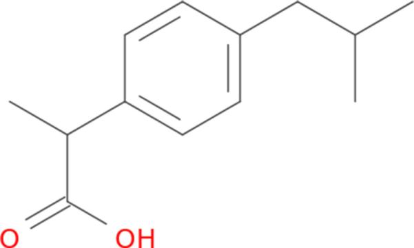
First-year chemistry students quickly become familiar with a common representation for small molecules: the molecular graph. Figure 1 gives an example of the molecular graph for ibuprofen, an over-the-counter non-steroidal anti-inflammatory drug. The atoms and bonds between atoms form the nodes and edges, respectively, of the graph. Both atoms and bonds have associated properties, such as atom type and bond order. Although the basic molecular graph representation does not capture the quantum mechanical structure of molecules or necessarily express all of the information that it might suggest to an expert medicinal chemist, its ubiquity in academia and industry makes it a desirable starting point for machine learning on chemical information.

Fig. 1.

Molecular graph for ibuprofen. Unmarked vertices represent carbon atoms, and bond order is indicated by the number of lines used for each edge

Here we describe molecular graph convolutions, a deep learning system using a representation of small molecules as undirected graphs of atoms. Graph convolutions extract meaningful features from simple descriptions of the graph structure—atom and bond properties, and graph distances—to form molecule-level representations that can be used in place of fingerprint descriptors in conventional machine learning applications.

Related work

The history of molecular representation is extremely diverse [38] and a full review is outside the scope of this report. Below we describe examples from several major branches of the field to provide context for our work. Additionally, we review several recent examples of graph-centric approaches in cheminformatics.

Much of cheminformatics is based on so-called “2D” molecular descriptors that attempt to capture relevant structural features derived from the molecular graph. In general, 2D features are computationally inexpensive and easy to interpret and visualize. One of the most common representations in this class is extended-connectivity fingerprints (ECFP), also referred to as circular or Morgan fingerprints [30]. Starting at each heavy atom, a “bag of fragments” is constructed by iteratively expanding outward along bonds (usually the algorithm is terminated after 2–3 steps). Each unique fragment is assigned an integer identifier, which is often hashed into a fixed-length representation or “fingerprint”. Additional descriptors in this class include decompositions of the molecular graph into sub-trees or fixed-length paths (OpenEye GraphSim Toolkit), as well as atom pair (AP) descriptors that encode atom types and graph distances (number of intervening bonds) for all pairs of atoms in a molecule [4].

Many representations encode 3D information, with special emphasis on molecular shape and electrostatics as primary drivers of interactions in real-world systems. For example, rapid overlay of chemical structures (ROCS) aligns pairs of pre-generated conformers and calculates shape and chemical (“color”) similarity using Gaussian representations of atoms and color features defined by a simple force field [11]. ROCS can also be used to generate alignments for calculation of electrostatic field similarity [23]. Ultrafast shape recognition (USR) calculates alignment-free 3D similarity by comparing distributions of intramolecular distances [2].

The Merck Molecular Activity Challenge [5] catalyzed interest in deep neural networks trained on fingerprints and other molecular descriptors. In particular, multitask neural networks have produced consistent gains relative to baseline models such as random forest and logistic regression [6, 17, 19, 29].

Other approaches from both the cheminformatics and the machine learning community directly operate on graphs in a way similar to how we do here. The “molecular graph networks” of Merkwirth and Lengauer [21] iteratively update a state variable on each atom with learned weights specific to each atom type–bond type pair. Similarly, Micheli [22] presents a more general formulation of the same concept of iterated local information transfer across edges and applies this method to predicting the boiling point of alkanes.

Scarselli et al. [33] similarly defines a local operation on the graph. They demonstrate that a fixed point across all the local functions can be found and calculate fixed point solutions for graph nodes as part of each training step. In another vein, Lusci et al. [16] convert undirected molecular graphs to a directed recursive neural net and take an ensemble over multiple conversions.

Recently, Duvenaud et al. [9] presented an architecture trying to accomplish many of the same goals as this work. The architecture was based on generalizing the fingerprint computation such that it can be learned via backpropagation. They demonstrate that this architecture improves predictions of solubility and photovoltaic efficiency but not binding affinity.

Bruna et al. [3] introduce convolutional deep networks on spectral representations of graphs. However, these methods apply when the graph structure is fixed across examples and only the labeling/features on individual nodes varies.

Convolutional networks on non-Euclidean manifolds were described by Masci et al. [18]. The problem addressed was to describe the shape of the manifold (such as the surface of a human being) in such a way that the shape descriptor of a particular point was invariant to perturbations such as movement and deformation. They also describe an approach for combining local shape descriptors into a global descriptor and demonstrate its use in a shape classification task.

Methods

Deep neural networks

Neural networks are directed graphs of simulated “neurons”. Each neuron has a set of inputs and computes an output. The neurons in early neural nets were inspired by biological neurons and computed an affine combination of the inputs followed by a non-linear activation function. Mathematically, if the inputs are x₁. . .x_N, weights w₁. . .w_N and bias b are parameters, and f is the activation function, the output is

$$f\left(b+\sum _i{w}_i{x}_i\right)$$ (1)

Popular activation functions include the sigmoid function $(f\left(z\right)=\frac{1}{1+e^{-z}})$ and rectified linear unit (ReLU) (f(z) = 0 if z ≤ 0 else z).

Any mostly differentiable function can be used as the unit of computation for a neuron and in recent years, many other functions have appeared in published networks, including max and sum.

Convolution in neural networks refers to using the same parameters (such as the w_i in Eq. 1) for different neurons that are attached to different parts of the input (or previous neurons). In this way, the same operation is computed for many different subsets of the input.

At the “top” of the neural network you have node(s) whose output is the value you are trying to predict (e.g. the probability that this molecule binds to a target or the binding affinity). Many output nodes for different tasks can be added and this is commonly done [17, 29]. In this way, different output tasks can share the computation and model parameters in lower parts of the network before using their own parameters for the final output steps.

The architecture of a neural network refers to the choice of the number of neurons, the type of computation each one does (including what learnable parameters they have), which parameters are shared across neurons, and how the output of one neuron is connected to the input of another.

In order to train the network, you first have to choose a loss function describing the penalty for the network producing a set of outputs which differ from the outputs in the training example. For example, for regression problems, the L2 distance between the predicted and actual values is commonly used. The objective of training is then to find a set of parameters for the network that minimizes the loss function. Training is done with the well known technique of back-propagation [32] and stochastic gradient descent.

Desired invariants of a model

A primary goal of designing a deep learning architecture is to restrict the set of functions that can be learned to ones that match the desired properties from the domain. For example, in image understanding, spatial convolutions force the model to learn functions that are invariant to translation.

For a deep learning architecture taking a molecular graph as input, some arbitrary choice must be made for the order that the various atoms and bonds are presented to the model. Since that choice is arbitrary, we want:

Property 1 (Order invariance) The output of the model should be invariant to the order that the atom and bond information is encoded in the input.

Note that many current procedures for fingerprinting molecules achieve Property 1. We will now gradually construct an architecture which achieves Property 1 while making available a richer space of learnable parameters.

The first basic unit of representation is an atom layer which contains an n-dimensional vector associated with each atom. Therefore the atom layer is a 2 dimensional matrix indexed first by atom. Part of the original input will be encoded in such an atom layer and the details of how we construct the original input vector are discussed in the “Input featurization” section. The next basic unit of representation is a pair layer which contains an n-dimensional vector associated with each pair of atoms. Therefore, the pair layer is a 3 dimensional matrix where the first two dimensions are indexed by atom. Note that the pair input can contain information not just about edges but about any arbitrary pair. Notably, we will encode the graph distance (length of shortest path from one atom to the other) in the input pair layer. The order of the atom indexing for the atom and pair layer inputs must be the same.

We will describe various operations to compute new atom and pair layers with learnable parameters at every step. Notationally, let A^x be the value of a particular atom layer x and P^y be the value of a particular pair layer y. The inputs that produce those values should be clear from the context. $A_a^x$ refers to the value of atom a in atom layer x and $P_{(a,b)}^y$ refers to the value of pair (a, b) in pair layer y.

In order to achieve Property 1 for the overall architecture, we need a different type of invariance for each atom and pair layer.

Property 2 (Atom and pair permutation invariance) The values of an atom layer and pair permute with the original input layer order. More precisely, if the inputs are permuted with a permutation operator Q, then for all layers x, y, A^x and P^y are permuted with operator Q as well.

In other words, Property 2 means that from a single atom's (or pair's) perspective, its value in every layer is invariant to the order of the other atoms (or pairs).

Since molecules are undirected graphs, we will also maintain the following:

Property 3 (Pair order invariance) For all pair layers y, $P_{(a,b)}^y=P_{(b,a)}^y$

Property 3 is easy to achieve at the input layer and the operations below will maintain this.

Properties 2 and 3 make it easy to construct a molecule-level representation from an atom or pair such that the molecule-level representation achieves Property 1 (see “Molecule-level features” section).

Invariant-preserving operations

We now define a series of operations that maintain the above properties.

Throughout, f represents an arbitrary function and g represents an arbitrary commutative function (g returns the same result regardless of the order the arguments are presented). In this work, f is a learned linear operator with a rectified linear (ReLU) activation function and g is a sum.

The most trivial operation is to combine one or more layers of the same type by applying the same operation to every atom or pair. Precisely, this means if you have layers x1, x2, . . ., xn and function f, you can compute a new atom layer from the previous atom layer (A → A) as

$$A_a^y=f\left(A_a^{x1},A_a^{x2},\dots ,A_a^{xn}\right)$$ (2)

or pair layer from the previous pair layer (P → P) as

$$P_{a,b}^y=f\left(P_{a,b}^{x1},P_{a,b}^{x2},\dots ,P_{a,b}^{xn}\right)$$ (3)

Since we apply the same function for every atom/pair, we refer to this as a convolution. All the transformations we develop below will have this convolution nature of applying the same operation to every atom/pair, maintaining Property 2.

When operating on pairs of atoms, instead of putting all pairs through this function, you could select a subset. In the “Distance-dependent pair features” section we show experiments for restricting the set of pairs to those that are less than some graph distance away.

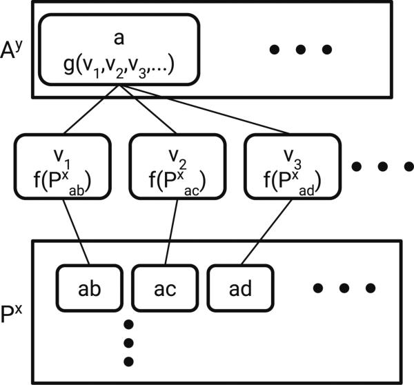
Next, consider an operation that takes a pair layer x and constructs an atom layer y (P → A). The operation is depicted in Fig. 2. Formally:

$$A_a^y=g\left(f\left(P_{(a,b)}^x\right),f\left(P_{(a,c)}^x\right),f\left(P_{(a,d)}^x\right),\dots \right)$$ (4)

In other words, take all pairs of which a is a part, run them through f, and combine them with g. Note that Property 3 means we can choose an arbitrary one of $P_{(a,b)}^x$ or $P_{(b,a)}^x$.

Fig. 2.

P → A operation. P^x is a matrix containing features for atom pairs ab, ac, ad, etc. The v_i are intermediate values obtained by applying f to features for a given atom pair. Applying g to the intermediate representations for all atom pairs involving a given atom (e.g. a) results in a new atom feature vector for that atom

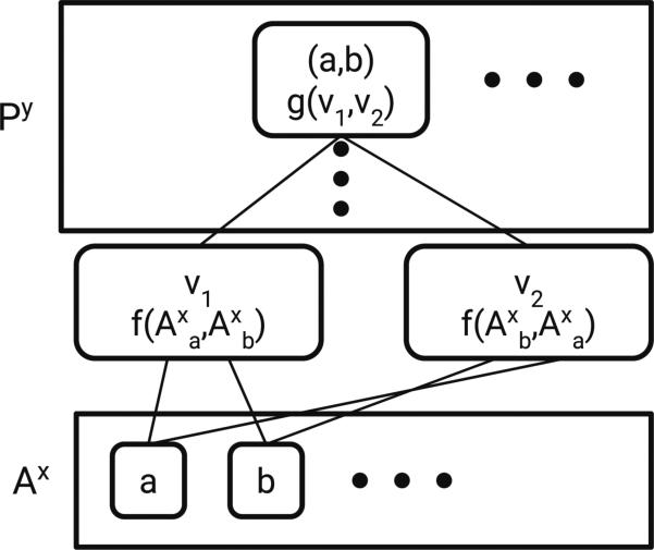
The most interesting construction is making a pair layer from an atom layer (A → P). The operation is graphically depicted in Fig. 3 and formally as

$$P_{ab}^y=g\left(f\left(A_a^x,A_b^x\right),f\left(A_b^x,A_a^x\right)\right)$$ (5)

Note that just applying g to $A_a^x$ and $A_b^x$ would maintain Properties 2 and 3 but we use this more complex form. While commutative operators (such as max pooling) are common in neural networks, commutative operators with learnable parameters are not common. Therefore, we use f to give learnable parameters while maintaining the desired properties.

Fig. 3.

A → P operation. A^x is a matrix containing features for atoms a, b, etc. The v_i are intermediate values obtained by applying f to features for a given pair of atoms concatenated in both possible orderings (ab and ba). Applying g to these intermediate ordered pair features results in an order-independent feature vector for atom pair ab

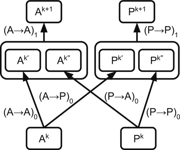
Once we have all the primitive operations on atom and pair layers (A → A, P →P, P → A, A → P), we can combine these into one module. We call this the Weave module (Fig. 4) because the atoms and pair layers cross back and forth to each other. The module can be stacked to an arbitrary depth similar to the Inception module that inspired it [37]. Deep neural networks with many layers (e.g. for computer vision) learn progressively more general features—combinations of lower-level features—in a hierarchical manner [15]. By analogy, successive Weave modules can produce more informative representations of the original input. Additionally, stacked Weave modules with limited maximum atom pair distance progressively incorporate longer-range information at each layer.

Fig. 4.

Weave module. This module takes matrices A^k and P^k (containing atom and pair features, respectively) and combines A → A, P → P, P → A, and A → P operations to yield a new set of atom and pair features (A^k+1 and P^k+1, respectively). The output atom and pair features can be used as input to a subsequent Weave module, which allows these modules to be stacked in series to an arbitrary depth

Molecule-level features

The construction of the Weave module maintains Properties 2 and 3. What about overall order invariance (Property 1)? At the end of a stack of Weave modules we are left with an n-dimensional vector associated with every atom and an m-dimensional vector associated with every pair. We need to turn this into a molecule-level representation with some commutative function of these vectors.

In related work [9, 16, 21], a simple unweighted sum is often used to combine order-dependent atom features into order-independent molecule-level features. However, reduction to a single value does not capture the distribution of learned features. We experimented with an alternative approach and created “fuzzy” histograms for each dimension of the feature vector.

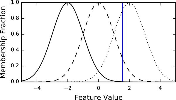
A fuzzy histogram is described by a set of membership functions that are functions with range [0, 1] representing the membership of the point in each histogram bin [42]. A standard histogram has membership functions which are 1 in the bin and 0 everywhere else. For each point, we normalize so that the total contribution to all bins is 1. The value of a bin in the histogram over all points is just the sum of the normalized contributions for all the points.

Figure 5 gives an example of a fuzzy histogram composed of three Gaussian bins. A histogram is constructed for each dimension of the feature vectors and the concatenation of those histograms is the molecule-level representation.

Fig. 5.

Fuzzy histogram with three Gaussian “bins”. Each curve represents the membership function for a different bin, indicating the degree to which a point contributes to that bin. The vertical blue line represents an example point which contributes normalized densities of <0:01, ~0:25, and ~0:75 to the bins (from left to right)

In this work we used Gaussian membership functions (which are unnormalized versions of the standard Gaussian PDF) with eleven bins spanning a Gaussian distribution with mean of zero and unit standard deviation, shown in Fig. S10. These bins were chosen somewhat arbitrarily to cover the expected distribution of incoming features and were not optimized further (note that the incoming features were batch normalized; see “Model training and evaluation” section).

Throughout this paper, we construct the molecule-level features only from the top-level atom features and not the pair features. This is to restrict the total number of feature vectors that must be summarized while still providing information about the entire molecule. Note, however, that the initial and intermediate pair features can influence the final atom features through Weave module operations.

Before the molecule-level featurization, we do one final convolution on the atoms. Since molecule-level featurization can be a major bottleneck in the model, this convolution expands the depth so that each dimension of the atom feature vector contains less information and therefore less information is lost during the molecule-level featurization. On this convolution, we do not use a ReLU activation function to avoid the histogram having many points at zero.

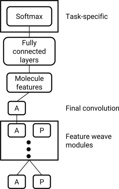
Once you have a molecule-level representation, this becomes a more standard multitask problem. We follow the common approach [17, 19, 29] of a small number of fully connected layers on top of the molecule-level features followed by standard softmax classification.

The overall architecture is depicted in Fig. 6. Table 1 lists hyperparameters and default values for graph convolution models. In models with multiple Weave modules it is conceivable to vary the convolution depths in a module-specific way. However, the models in this work used the same settings for all Weave modules.

Fig. 6.

Abstract graph convolution architecture. In the current implementation, only the final atom features are used to generate molecule-level features

Table 1.

Graph convolution model hyperparameters

Group	Hyperparameter	Default value
Input	Maximum number of atoms per molecule	60
	Maximum atom pair graph distance	2
Weave	Number of Weave modules	1
	(A → A)0 convolution depth	50
	(A → P)0 convolution depth	50
	(P → P)0 convolution depth	50
	(P → A)0 convolution depth	50
	(A → A)1 convolution depth	50
	(P → P)1 convolution depth	50
Reduction	Final atom layer convolution depth	128
	Reduction to molecule-level features	Gaussian histogram
Post-reduction	Fully-connected layers (number of units per layer)	2000, 100
Training	Batch size	96
	Learning rate	0.003
	Optimization method	Adagrad

Our current implementation imposes an upper limit on the number of heavy atoms represented in the initial featurization. For molecules that have more than the maximum number of atoms, only a subset of atoms (and therefore atom pairs) are represented in the input encoding. This subset depends on the order in which the atoms are traversed by the featurization code and should be considered arbitrary. In this work we set the maximum number of atoms to 60, and only 814 of the 1,442,713 unique molecules in our datasets (see “Datasets” section) exceed this limit.

Input featurization

The initial atom and pair features are summarized in Tables 2 and 3, respectively. The features are a mix of floating point, integer, and binary values (all encoded as floating point numbers in the network). The feature set is intended to be broad, but not necessarily exhaustive, and we recognize that some features can potentially be derived from or correlated to a subset of the others (e.g. atom hybridization can be determined by inspecting the bonds that atom makes). We performed experiments using a “simple” subset of these features in an effort to understand their relative contributions to learning (“Input featurization” section), but many other questions about specifics of the input featurization are left to future work.

Table 2.

Atom features

Feature	Description	Size
Atom typea	H, C, N, O, F, P, S, Cl, Br, I, or metal (one-hot or null)	11
Chirality	R or S (one-hot or null)	2
Formal charge	Integer electronic charge	1
Partial charge	Calculated partial charge	1
Ring sizes	For each ring size (3–8), the number of rings that include this atom	6
Hybridization	sp, sp2, or sp3 (one-hot or null)	3
Hydrogen bonding	Whether this atom is a hydrogen bond donor and/or acceptor (binary values)	2
Aromaticity	Whether this atom is part of an aromatic system	1
		27

^aIncluded in the “simple” featurization (see “Input featurization” section)

Table 3.

Atom pair features

Feature	Description	Size
Bond typea	Single, double, triple, or aromatic (one-hot or null)	4
Graph distancea	For each distance (1–7), whether the shortest path between the atoms in the pair is less than or equal to that number of bonds (binary values)	7
Same ring	Whether the atoms in the pair are in the same ring	1
		12

^aIncluded in the “simple” featurization (see “Input featurization” section)

All features were generated with RDKit [14], including Gasteiger atomic partial charges [10]. Although our featurization includes space for hydrogen atoms, we did not use explicit hydrogens in any of our experiments in order to conserve memory and emphasize contributions from heavy atoms.

Other deep learning applications with more “natural” inputs such as computer vision and speech recognition still require some input engineering; for example, adjusting images to a specific size or scale, or transforming audio into the frequency domain. Likewise, the initial values for the atom and pair layers describe these primitives in terms of properties that are often considered by medicinal chemists and other experts in the field, allowing the network to use or ignore them as needed for the task at hand. One of the purposes of this work is to demonstrate that learning can occur with as little preprocessing as possible. Accordingly, we favor simple descriptors that are more or less “obvious”.

Datasets

We used a dataset collection nearly identical to the one described by Ramsundar et al. [29] except for some changes to the data processing pipeline (including the duplicate merging process for the Tox21 dataset) and different cross-validation fold divisions. Briefly, there are 259 datasets divided into four groups indicating their source: PubChem BioAssay [41] (PCBA, 128 datasets), the “maximum unbiased validation” datasets constructed by Rohrer and Baumann [31] (MUV, 17 datasets), the enhanced directory of useful decoys [24] (DUD-E, 102 datasets), and the training set for the Tox21 challenge (see Mayr et al. [19]) (Tox21, 12 datasets). The combined dataset contained over 38 M data points and included targets from many different biological classes.

Model training and evaluation

Graph convolution and traditional neural network models were implemented with TensorFlow [1], an open-source library for machine learning. Models were evaluated by the area under the receiver operating characteristic curve (ROC AUC, or simply AUC) as recommended by Jain and Nicholls [13]. We used fivefold stratified cross-validation, where each fold-specific model used 60 % of the data for training, 20 % for validation (early stopping/model selection), and 20 % as a test set.

Graph convolution models were trained for 10–20 M steps using the Adagrad optimizer [8] with learning rate 0.003 and batch size 96, with periodic checkpointing. All convolution and fully-connected layer outputs were batch normalized [12] prior to applying the ReLU nonlinearity. Training was parallelized over 96 CPUs (or 96 GPUs in the case of the W₄N₂ model) and required several days for each model. Adding additional Weave modules significantly increased training time. However, models trained on smaller datasets (see “Comparisons to other methods” section) trained much faster.

To establish a baseline, we also trained pyramidal (2000, 100) multitask neural network (PMTNN) [29], random forest (RF), and logistic regression (LR) models using Morgan fingerprints with radius 2 (essentially equivalent to ECFP4) generated with RDKit [14]. As a very simple baseline, we also computed Tanimoto similarity to all training set actives and used the maximum similarity score as the active class probability (MaxSim).

The PMTNN had two hidden layers (with 2000 and 100 units, respectively) with rectified linear activations, and each fold-specific model was trained for 40–50 M steps using the SGD optimizer with batch size 128 and a learning rate of 0.0003, with periodic checkpointing. Additionally, this model used 0.25 dropout [35], initial weight standard deviations of 0.01 and 0.04 and initial biases of 0.5 and 3.0 in the respective hidden layers. This model did not use batch normalization.

Logistic regression (LR) models were trained with the LogisticRegression class in scikit-learn [27] using the ‘lbfgs’ solver and a maximum of 10,000 iterations. Values for the regularization strength (C) parameter were chosen by grid search, using the held-out validation set for model selection. Random forest (RF) models were trained using the scikit-learn RandomForestClassifier with 100 trees.

In graph convolution and PMTNN models, active compounds were weighted in the cost function such that the total active weight equalled the total inactive weight within each dataset (logistic regression and random forest models also used these weights as the sample_weight argument to their fit methods). Furthermore, graph convolution and PMTNN models were evaluated in a task-specific manner by choosing the training checkpoint with the best validation set AUC for each task. We note that some fold-specific models had a small number of tasks were not “converged” in the sense that their validation set AUC scores were still increasing when training was halted, and that the specific tasks that were not converged varied from model to model.

To statistically compare graph convolution and baseline models, we report three values for each dataset group: (1) median fivefold mean AUC over all datasets, (2) median difference in per-dataset fivefold mean AUC (ΔAUC) relative to the PMTNN baseline, and (3) a 95 % Wilson score interval for the sign test statistic relative to the PMTNN baseline. The sign test estimates the probability that a model will achieve a higher fivefold mean AUC than the PMTNN baseline; models with sign test confidence intervals that do not include 0.5 are considered significantly different in their performance (the median ΔAUC can be used as a measure of effect size). To calculate these intervals, we used the proportion_confint function in statsmodels [34] version 0.6.1 with method=‘wilson’ and alpha=0.05, counting only non-zero differences in the sign test. We do not report values for the DUD-E dataset group since all models achieved >0.98 median fivefold mean AUC.

As a general note, confidence intervals for box medians were computed as $\pm 1.57\times \mathrm{IQR}∕\sqrt{\mathrm{N}}$ [20] and do not necessarily correspond to sign test confidence intervals.

Comparisons to other methods

In addition to the baseline models described in the “Model training and evaluation” section, there are many other methods that would be interesting to compare to our graph convolution models. In particular, Duvenaud et al. [9] described “neural fingerprints” (NFP), a related graph-based method. The original publication describing NFP reported mean squared errors (MSE) on datasets for aqueous solubility, drug efficacy, and photovoltaic efficiency. We trained multitask graph convolution models on these datasets using fivefold cross-validation (note that the published NFP models were single-task).

Additionally, we report results on a dataset used to validate the influence relevance voter (IRV) method of Swamidass et al. [36], which is a hybrid of neural networks and k-nearest neighbors. The original publication reported results for two datasets, HIV and DHFR, but the latter was no longer available from its original source. We trained graph convolution models on the HIV dataset using tenfold stratified cross-validation. In each cross-validation round, onefold each was used for testing and validation (early stopping), and the remaining folds were used for training. We note that RDKit was only able to process 41,476 of the 42,678 SMILES strings in the HIV dataset. We report performance on this dataset using both ROC AUC and BEDROC [39] with α = 20.

Although we expect our results on these datasets to provide reasonable comparisons to published data, differences in fold assignments and variations in dataset composition due to featurization failures mean that the comparisons are not perfect.

Results

Proof of concept

With so many hyperparameters to adjust, we sought to establish a centerpoint from which to investigate specific questions. After several experiments, we settled on a simple model with two Weave modules, a maximum atom pair distance of 2, Gaussian histogram molecule-level reductions, and two fully-connected layers of size 2000 and 100, respectively. Notationally, we refer to this model as W₂N₂. Table 4 shows the performance of the W₂N₂ model and related models derived from this centerpoint by varying a single hyperparameter. Additionally, Table 4 includes results for several baseline models: MaxSim, logistic regression (LR), random forest (RF), and pyramidal (2000, 100) multitask neural network (PMTNN) models trained on Morgan fingerprints.

Table 4.

Median fivefold mean AUC values for reported models

Model	PCBA (n = 128)			MUV (n = 17)			Tox21 (n = 12)
	Median AUC	Median ΔAUC	Sign Test 95% CI	Median AUC	Median ΔAUC	Sign Test 95% CI	Median AUC	Median ΔAUC	Sign Test 95% CI
MaxSim	0.754	−0.137	(0.00, 0.04)	0.638	−0.136	(0.01, 0.27)	0.728	−0.131	(0.00, 0.24)
LR	0.838	−0.059	(0.04, 0.13)	0.736	−0.070	(0.10, 0.47)	0.789	−0.073	(0.01, 0.35)
RF	0.804	−0.092	(0.02, 0.10)	0.655	−0.135	(0.01, 0.27)	0.802	−0.047	(0.01, 0.35)
PMTNN	0.905			0.869			0.854
W2N2-simple	0.905	−0.003	(0.27, 0.44)	0.849	0.012	(0.36, 0.78)	0.866	0.003	(0.39, 0.86)
W2N2-sum	0.898	−0.011	(0.16, 0.31)	0.818	−0.014	(0.17, 0.59)	0.848	−0.010	(0.09, 0.53)
W2N2-RMS	0.902	−0.007	(0.20, 0.35)	0.851	−0.026	(0.13, 0.53)	0.854	−0.007	(0.05, 0.45)
W1N2	0.905	−0.007	(0.20, 0.35)	0.840	−0.002	(0.26, 0.69)	0.849	−0.009	(0.09, 0.53)
W2N1	0.908	−0.003	(0.30, 0.46)	0.858	−0.016	(0.17, 0.59)	0.867	−0.002	(0.19, 0.68)
W2N2	0.909	0.000	(0.42, 0.59)	0.847	−0.004	(0.22, 0.64)	0.862	0.004	(0.32, 0.81)
W2N3	0.906	−0.001	(0.38, 0.55)	0.838	−0.013	(0.26, 0.69)	0.861	0.000	(0.25, 0.75)
W2N4	0.908	−0.001	(0.37, 0.54)	0.836	−0.008	(0.17, 0.59)	0.858	0.001	(0.39, 0.86)
W2N∞	0.897	−0.008	(0.12, 0.25)	0.841	−0.025	(0.10, 0.47)	0.846	−0.006	(0.14, 0.61)
W3N2	0.906	0.000	(0.44, 0.61)	0.875	0.010	(0.31, 0.74)	0.859	0.004	(0.47, 0.91)
W4N2	0.907	−0.001	(0.33, 0.50)	0.856	−0.007	(0.22, 0.64)	0.862	0.004	(0.32, 0.81)

Graph convolution models are labeled as W_xN_y, where x and y denote the number of Weave modules and the maximum atom pair distance, respectively (see the text for descriptions of the simple, sum, and RMS models). All graph convolution models fed into a Pyramidal (2000, 100) MTNN after the molecule-level feature reduction step. MaxSim, logistic regression (LR), random forest (RF), and pyramidal (2000, 100) multitask neural network (PMTNN) baselines used Morgan fingerprints as input. For each model, we report the median ΔAUC and the 95 % Wilson score interval for a sign test estimating the probability that a given model will outperform the PMTNN baseline (see “Model training and evaluation” section). Bold values indicate sign test confidence intervals that do not include 0.5

Several graph convolution models achieved performance comparable to the baseline PMTNN on the classification tasks in our dataset collection, which is a remarkable result considering the simplicity of our input representation. For example, the centerpoint W₂N₂ model is statistically indistinguishable from the PMTNN for the PCBA, MUV, and Tox21 dataset groups (we do not report results for the DUD-E dataset group because all models achieved extremely high median AUC scores). Additionally, many of the graph convolution models with worse performance than the PMTNN (i.e. sign test confidence intervals excluding 0.5) had very small effective differences as measured by median ΔAUC.

As an additional measure of model performance, we also calculated ROC enrichment [13] scores at the following false positive rates: 1, 5, 10, and 20 %. Enrichment scores are reported in Section B (in the supplementary material) and show that graph convolution models generally performed worse than or comparable to the PMTNN. We note that the analysis of model performance and hyperparameter optimization that follows is based only on ROC AUC scores.

We also trained graph convolution models on some additional datasets in order to compare to the “neural fingerprints” (NFP) of Duvenaud et al. [9] and the influence relevance voter (IRV) method of Swamidass et al. [36] (see “Comparisons to other methods” section). Table 5 compares graph convolution models to published results on these datasets under similar cross-validation conditions. Graph convolution results were comparable to published NFP models, with significant improvement on the photo-voltaic efficiency task (note that the graph convolution results are from multitask models trained on all three NFP datasets while Duvenaud et al. [9] report values for single-task models). The tenfold mean AUC and BEDROC scores on the HIV dataset were slightly lower than the published IRV values. However, we held out 10 % of the data (one fold) in each cross-validation round as a validation set for checkpoint selection, meaning that the graph convolution models were trained with fewer examples than the published IRV models.

Table 5.

Comparison of graph convolution to neural fingerprint (NFP) and influence relevance voter (IRV) models

Model	Dataset	Metric	Original	Graph convolution
NFP	Solubility (log M)	MSE	0.52 ± 0.07	0.46 ± 0.08
	Drug efficacy (nM EC50)	MSE	1.16 ± 0.03	1.07 ± 0.06
	Photovoltaic efficiency (%)	MSE	1.43 ± 0.09	1.10 ± 0.06
IRV	HIV	AUC	0.845	0.838 ± 0.027
		BEDROC (α = 20)	0.630	0.613 ± 0.048

Section “Comparisons to other methods” provides details for datasets and experimental procedures. Note that the NFP comparisons were performed using multitask graph convolution models, and that graph convolution models for the HIV dataset were trained with fewer examples than IRV since one cross-validation fold was used as a held-out validation set

Input featurization

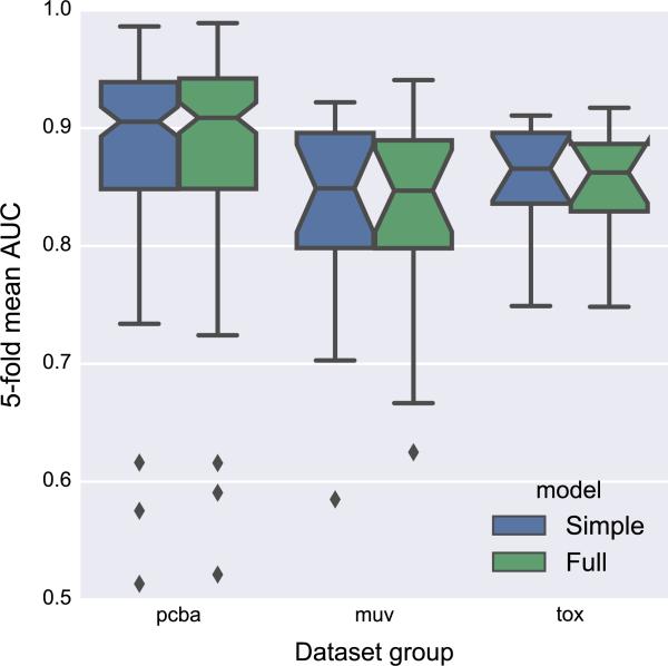
As a further proof of concept and to address the importance of the initial featurization, we trained a model using a subset of features that match typical 2D structural diagrams seen in chemistry textbooks: only atom type, bond type, and graph distance are provided to the network. Figure 7 compares a model trained with this “simple” input featurization to the “full” featurization containing all features from Table 2 and Table 3. Both featurizations achieve similar median fivefold mean AUC scores, suggesting that the additional features in the “full” representation are either mostly ignored during training or can be derived from a simpler representation of the molecular graph. Further work is required to understand the importance of individual features, perhaps with datasets that are sensitive to particular components of the input representation (such as hydrogen bonding or formal charge).

Fig. 7.

Comparison of models with “simple” and “full” input featurizations. The simple featurization only encodes atom type, bond type, and graph distance. The full featurization includes additional features such as aromaticity and hydrogen bonding propensity (see “Molecule-level features” section for more details). Confidence intervals for box plot medians were computed as $\pm 1.57\times \mathrm{IQR}∕\sqrt{\mathrm{N}}$ [20]

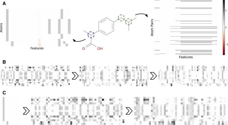
Figure 8 gives examples of how the initial atom features for a single molecule (ibuprofen) evolve as they progress through graph convolution Weave modules. The initial atom and pair feature encodings for the “full” featurization are depicted in Panel A. Comparing the initial atom features to their source molecular graph, the aromatic carbons in the central ring are clearly visible (and nearly identical in the featurization). The pair features are more difficult to interpret visually, and mostly encode graph distance. As the atom features are transformed by the Weave modules (Panel B), they become more heterogeneous and reflective of their unique chemical environments. “Simple” features behave similarly, beginning with rather sterile initial values and quickly diverging as neighborhood information is included by Weave module operations (Panel C). Comparison of the “full” and “simple” atom features after the second Weave module shows that both featurizations lead to similarly diverse feature distributions. Fig. S8 and Fig. S9 show similar behavior for pair features.

Fig. 8.

Graph convolution feature evolution. Atoms or pairs are displayed on the y-axis and the dimensions of the feature vectors are on the x-axis. a Conversion of the molecular graph for ibuprofen into atom and (unique) atom pair features. b Evolution of atom features after successive Weave modules in a graph convolution model with a W₃N₂ architecture and depth 50 convolutions in Weave modules. c Evolution of “simple” atom features (see “Input featurization” section) starting from initial encoding and progressing through the Weave modules of a W₂N₂ architecture. The color bar applies to all panels

Hyperparameter sensitivity

Number of Weave modules

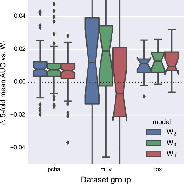
In relatively “local” models with limited atom pair distance, successive Weave modules update atom features with information from progressively larger regions of the molecule. This suggests that the number of Weave modules is a critical hyperparameter to optimize, analogous to the number of hidden layers in traditional neural networks. Figure 9 compares models with 2–4 Weave modules to a model with a single Weave module. As expected, models with a single Weave layer were outperformed by deeper architectures. For the PCBA and Tox21 datasets, there was not much benefit to using more than two Weave modules (Fig. S5), but using three Weave modules gave the best median AUC for the MUV datasets (in exchange for significantly increased training time).

Fig. 9.

Comparison of models with different numbers of Weave modules with a model containing a single Weave module. All models used a maximum atom pair distance of two. The y-axis is cropped to emphasize differences near zero

Alternative feature reductions

The reduction of atom features from the final Weave module to an order-invariant, molecule-level representation is a major information bottleneck in graph convolution models. In related work, a simple unweighted sum [9, 16, 21] or root-mean-square (RMS) [7] reduction is used. Using a consistent base architecture with two Weave modules and a maximum atom pair distance of 2, we compared these traditional reduction strategies with our Gaussian histogram approach.

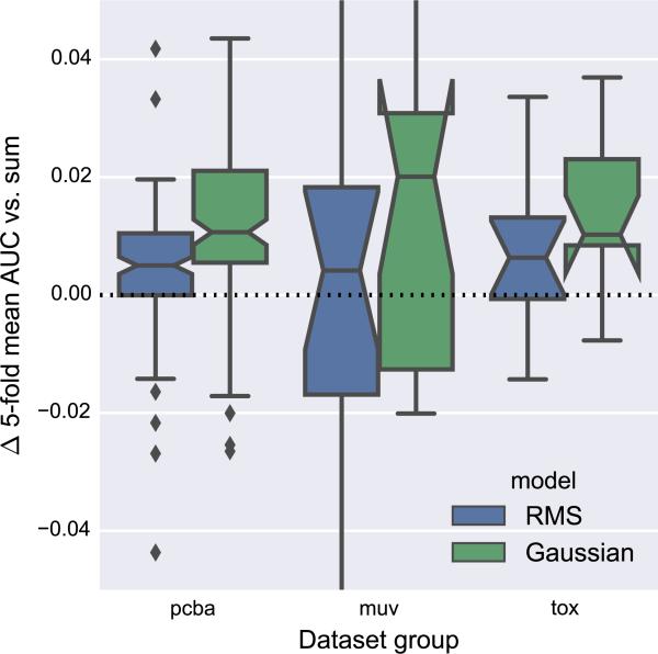
Figure 10 shows that Gaussian histogram models had consistently improved scores relative to sum reductions. RMS reductions were not as robust as Gaussian histograms in terms of per-dataset differences relative to sum reductions, although RMS and Gaussian histogram reductions had similar distributions of absolute AUC values (Fig. S6). Additionally, RMS reductions achieved a slightly higher median AUC than Gaussian histogram reductions on the MUV datasets.

Fig. 10.

Comparison of root-mean-square (RMS) and Gaussian histogram reductions versus sum reduction. The y-axis reports difference in fivefold mean AUC relative to sum reduction. All models used two Weave modules and a maximum atom pair distance of two. The y-axis is cropped to emphasize differences near zero

Distance-dependent pair features

In Weave modules, atoms are informed about their chemical environment by mixing with pair features in the P → A operation. Recall that during this operation, pair features are combined for pairs that contain a given atom, yielding a new representation for that atom. A critical parameter for this operation is the maximum distance (in bonds) allowed between the atoms of the pairs that are combined. If only adjacent atoms are combined, the resulting atom features will reflect the local chemical environment. As an alternative to increasing the number of Weave modules, longer-range interactions can be captured by increasing the maximum atom pair distance. However, our implementation of the P → A operation uses a simple sum to combine pair features, such that a large amount of information (possibly including every pair of atoms in the molecule) is combined in a way that could prevent useful information from being available in later stages of the network.

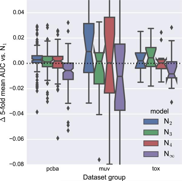
Figure 11 shows the performance of several models with different maximum pair distances relative to a model that used only adjacent atom pairs (N₁). For the PCBA datasets, a maximum distance of 2 (N₂) improves performance to relative the N₁ model, and N_∞ (no maximum distance) is clearly worse. However, the N₁ model achieves the best median AUC score for the MUV and Tox21 datasets (Table 4 and Fig. S7). These results suggest that graph convolution models do not effectively make use of the initial graph distance features to preserve or emphasize distance-dependent information.

Fig. 11.

Comparison of models with different maximum atom pair distances to a model with a maximum pair distance of one (bonded atoms). All models have two Weave modules. The y-axis is cropped to emphasize differences near zero

To further investigate the effect of distance information in Weave modules, we experimented with models that use distance-specific weights for operations involving pair features in order to maintain distance information explicitly throughout the network. However, results for these models are preliminary and were not included in this report.

Discussion

Graph convolutions are a deep learning architecture for learning directly from undirected graphs. In this work, we emphasize their application to small molecules—undirected graphs of atoms connected by bonds—for virtual screening. Starting from simple descriptions of atoms, bonds between atoms, and pairwise relationships in a molecular graph, we have demonstrated performance that is comparable to state of the art multitask neural networks trained on traditional molecular fingerprint representations, as well as alternative methods including “neural fingerprints” [9] and influence relevance voter [36].

Our experiments with the adjustable parameters in graph convolution models indicate a relatively minor sensitivity to the number of Weave modules and the maximum distance between atom pairs (at least for our datasets). These results suggest that a model with two Weave modules, a maximum atom pair distance of 2, and Gaussian histogram reductions is a good starting point for further optimization. Remarkably, graph convolution models perform well with a “simple” input featurization containing only atom type, bond type, and graph distances—essentially the information available from looking at Fig. 1.

Flexibility is a highlight of the graph convolution architecture: because we begin with a representation that encodes the complete molecular graph, graph convolution models are free to use any of the available information for the task at hand. In a sense, every possible molecular “fingerprint” is available to the model. Said another way, graph convolutions and other graph-based approaches purposefully blur the distinction between molecular features and predictive models. As has been pointed out elsewhere [9], the ability to use backpropagation to tune parameters at every stage of the network provides greater representational power than traditional descriptors, which are inflexible in the features they encode from the initial representation. Accordingly, it is not appropriate to think of graph-based methods as alternative descriptors; rather, they should be viewed as fully integrated approaches to virtual screening (although future work could investigate the utility of the learned molecule-level features for additional tasks or other applications such as molecular similarity).

Looking forward, graph convolutions (and related graph-based methods; see “Related work” section) present a “new hill to climb” in computer-aided drug design and cheminformatics. Although our current graph convolution models do not consistently outperform state-of-the-art fingerprint-based models, we emphasize their flexibility and potential for further optimization and development. In particular, we are aware of several specific opportunities for improvement, including (1) additional optimization of model hyperparameters such as Weave module convolution depths; (2) fine-tuning of architectural decisions, such as the choice of reduction in the P → A operation (currently a sum, but perhaps a Gaussian histogram or distance-dependent function); and (3) improvements in memory usage and training performance, such as not handling all pairs of atoms or implementing more efficient versions of Weave module operations. With these and other optimizations, we expect that graph convolutions could exceed the performance of the best available fingerprint-based methods.

Finally, we note that much (or most) of the information required to represent biological systems and the interactions responsible for small molecule activity is not encapsulated in the molecular graph. Biology takes place in a three-dimensional world, and is sensitive to shape, electrostatics, quantum effects, and other properties that emerge from—but are not necessarily unique to—the molecular graph (see, for example, Nicholls et al. [25]). Additionally, most small molecules exhibit 3D conformational flexibility that our graph representation does not even attempt to describe. The extension of deep learning methods (including graph convolutions) to three-dimensional biology is an active area of research (e.g. Wallach et al. [40]) that requires special attention to the added complexities of multiple-instance learning in a relatively small-data regime.

References

- 1.Abadi M, Agarwal A, Barham P, Brevdo E, Chen Z, Citro C, Corrado GS, Davis A, Dean J, Devin M, et al. TensorFlow: large-scale machine learning on heterogeneous systems. Software. 2015 http://tensorflow.org.
- 2.Ballester PJ, Richards WG. Ultrafast shape recognition to search compound databases for similar molecular shapes. J Comput Chem. 2007;28(10):1711–1723. doi: 10.1002/jcc.20681. [DOI] [PubMed] [Google Scholar]
- 3.Bruna J, Zaremba W, Szlam A, LeCun Y. Spectral networks and locally connected networks on graphs. arXiv. 2013:1312–6203. [Google Scholar]
- 4.Carhart RE, Smith DH, Venkataraghavan R. Atom pairs as molecular features in structure-activity studies: definition and applications. J Chem Inf Comput Sci. 1985;25(2):64–73. [Google Scholar]
- 5.Dahl G. Deep learning how I did it: Merck 1st place interview. 2012 http://blog.kaggle.com/2012/11/01/deep-learning-how-i-did-it-merck-1st-place-interview.
- 6.Dahl GE, Jaitly N, Salakhutdinov R. Multi-task neural networks for QSAR predictions. 2014 arXiv:1406.1231. [Google Scholar]
- 7.Dieleman S. Classifying plankton with deep neural networks. 2015 Mar 17; 2015. http://benanne.github.io/2015/03/17/plankton.html.
- 8.Duchi J, Hazan E, Singer Y. Adaptive subgradient methods for online learning and stochastic optimization. J Mach Learn Res. 2011;12:2121–2159. [Google Scholar]
- 9.Duvenaud DK, Maclaurin D, Iparraguirre J, Bombarell R, Hirzel T, Aspuru-Guzik A, Adams RP. Convolutional networks on graphs for learning molecular fingerprints. Advances in neural information processing systems. 2015:2224–2232. [Google Scholar]
- 10.Gasteiger J, Marsili M. Iterative partial equalization of orbital electronegativity–a rapid access to atomic charges. Tetrahedron. 1980;36(22):3219–3228. [Google Scholar]
- 11.Hawkins PCD, Skillman AG, Nicholls A. Comparison of shape-matching and docking as virtual screening tools. J Med Chem. 2007;50(1):74–82. doi: 10.1021/jm0603365. [DOI] [PubMed] [Google Scholar]
- 12.Ioffe S, Szegedy C. Batch normalization: accelerating deep network training by reducing internal covariate shift. 2015 arXiv:1502.03167. [Google Scholar]
- 13.Jain AN, Nicholls A. Recommendations for evaluation of computational methods. J Comput Aided Mol Des. 2008;22(3–4):133–139. doi: 10.1007/s10822-008-9196-5. [DOI] [PMC free article] [PubMed] [Google Scholar]
- 14.Landrum G. RDKit: open-source cheminformatics. 2014 http://www.rdkit.org.
- 15.LeCun Y, Bengio Y, Hinton G. Deep learning. Nature. 2015;521(7553):436–444. doi: 10.1038/nature14539. [DOI] [PubMed] [Google Scholar]
- 16.Lusci A, Pollastri G, Baldi P. Deep architectures and deep learning in chemoinformatics: the prediction of aqueous solubility for drug-like molecules. J Chem Inf Model. 2013;53(7):1563–1575. doi: 10.1021/ci400187y. [DOI] [PMC free article] [PubMed] [Google Scholar]
- 17.Ma J, Sheridan RP, Liaw A, Dahl GE, Svetnik V. Deep neural nets as a method for quantitative structure–activity relationships. J Chem Inf Model. 2015;55(2):263–274. doi: 10.1021/ci500747n. [DOI] [PubMed] [Google Scholar]
- 18.Masci J, Boscaini D, Bronstein M, Vandergheynst P. Geodesic convolutional neural networks on riemannian manifolds. Proceedings of the IEEE international conference on computer vision workshops. 2015:37–45. [Google Scholar]
- 19.Mayr A, Klambauer G, Unterthiner T, Hochreiter S. Deeptox: toxicity prediction using deep learning. Front Environ Sci. 2015;3:80. [Google Scholar]
- 20.McGill R, Tukey JW, Larsen WA. Variations of box plots. Am Stat. 1978;32(1):12–16. [Google Scholar]
- 21.Merkwirth C, Lengauer T. Automatic generation of complementary descriptors with molecular graph networks. J Chem Inf Model. 2005;45(5):1159–1168. doi: 10.1021/ci049613b. [DOI] [PubMed] [Google Scholar]
- 22.Micheli A. Neural network for graphs: a contextual constructive approach. IEEE Trans Neural Netw. 2009;20(3):498–511. doi: 10.1109/TNN.2008.2010350. [DOI] [PubMed] [Google Scholar]
- 23.Muchmore SW, Souers AJ, Akritopoulou-Zanze I. The use of three-dimensional shape and electrostatic similarity searching in the identification of a melanin-concentrating hormone receptor 1 antagonist. Chem Biol Drug Des. 2006;67(2):174–176. doi: 10.1111/j.1747-0285.2006.00341.x. [DOI] [PubMed] [Google Scholar]
- 24.Mysinger MM, Carchia M, Irwin JJ, Shoichet BK. Directory of useful decoys, enhanced (DUD-E): better ligands and decoys for better benchmarking. J Med Chem. 2012;55(14):6582–6594. doi: 10.1021/jm300687e. [DOI] [PMC free article] [PubMed] [Google Scholar]
- 25.Nicholls A, McGaughey GB, Sheridan RP, Good AC, Warren G, Mathieu M, Muchmore SW, Brown SP, Grant JA, Haigh JA, et al. Molecular shape and medicinal chemistry: a perspective. J Med Chem. 2010;53(10):3862–3886. doi: 10.1021/jm900818s. [DOI] [PMC free article] [PubMed] [Google Scholar]
- 26.OpenEye GraphSim Toolkit. OpenEye Scientific Software; Santa Fe, NM.: http://www.eyesopen.com. [Google Scholar]
- 27.Pedregosa F, Varoquaux G, Gramfort A, Michel V, Thirion B, Grisel O, Blondel M, Prettenhofer P, Weiss R, Dubourg V, et al. Scikit-learn: machine learning in python. J Mach Learn Res. 2011;12:2825–2830. [Google Scholar]
- 28.Petrone PM, Simms B, Nigsch F, Lounkine E, Kutchukian P, Cornett A, Deng Z, Davies JW, Jenkins JL, Glick M. Rethinking molecular similarity: comparing compounds on the basis of biological activity. ACS Chem Biol. 2012;7(8):1399–1409. doi: 10.1021/cb3001028. [DOI] [PubMed] [Google Scholar]
- 29.Ramsundar B, Kearnes S, Riley P, Webster D, Konerding D, Pande V. Massively multitask networks for drug discovery. 2015 arXiv:1502.02072. [Google Scholar]
- 30.Rogers D, Hahn M. Extended-connectivity fingerprints. J Chem Inf Model. 2010;50(5):742–754. doi: 10.1021/ci100050t. [DOI] [PubMed] [Google Scholar]
- 31.Rohrer SG, Baumann K. Maximum unbiased validation (MUV) data sets for virtual screening based on pubchem bioactivity data. J Chem Inf Model. 2009;49(2):169–184. doi: 10.1021/ci8002649. [DOI] [PubMed] [Google Scholar]
- 32.Rumelhart DE, Hinton GE, Williams RJ. Learning representations by back-propagating errors. Nature. 1986;323:533–536. [Google Scholar]
- 33.Scarselli F, Gori M, Tsoi AC, Hagenbuchner M, Monfardini G. The graph neural network model. IEEE Trans Neural Netw. 2009;20(1):61–80. doi: 10.1109/TNN.2008.2005605. [DOI] [PubMed] [Google Scholar]
- 34.Seabold S, Perktold J. Statsmodels: econometric and statistical modeling with python. Proceedings of the 9th Python in science conference. 2010:57–61. [Google Scholar]
- 35.Srivastava N, Hinton G, Krizhevsky A, Sutskever I, Salakhutdinov R. Dropout: a simple way to prevent neural networks from overfitting. J Mach Learn Res. 2014;15(1):1929–1958. [Google Scholar]
- 36.Swamidass JS, Azencott C-A, Lin T-W, Gramajo H, Tsai S-C, Baldi P. Influence relevance voting: an accurate and interpretable virtual high throughput screening method. J Chem Inf Model. 2009;49(4):756–766. doi: 10.1021/ci8004379. [DOI] [PMC free article] [PubMed] [Google Scholar]
- 37.Szegedy C, Liu W, Jia Y, Sermanet P, Reed S, Anguelov D, Erhan D, Vanhoucke V, Rabinovich A. Going deeper with convolutions. CVPR 2015. 2015 arxiv.org/abs/1409.4842. [Google Scholar]
- 38.Todeschini R, Consonni V. Molecular descriptors for chemoinformatics. Vol. 41. Wiley; New York: 2009. volume 41 (2 volume set) [Google Scholar]
- 39.Truchon J-F, Bayly CI. Evaluating virtual screening methods: good and bad metrics metrics for the âĂIJearly recog nitionâĂİ problem. J Chem Inf Model. 2007;47(2):488–508. doi: 10.1021/ci600426e. [DOI] [PubMed] [Google Scholar]
- 40.Wallach I, Dzamba M, Heifets A. AtomNet: a deep convolutional neural network for bioactivity prediction in structure-based drug discovery. 2015 arXiv:1510.02855. [Google Scholar]
- 41.Yanli W, Xiao J, Suzek TO, Zhang J, Wang J, Zhou Z, Han L, Karapetyan K, Dracheva S, Shoemaker BA, et al. Pub-Chem's BioAssay database. Nucl Acids Res. 2012;40(D1):D400–D412. doi: 10.1093/nar/gkr1132. [DOI] [PMC free article] [PubMed] [Google Scholar]
- 42.Zadeh LA. Fuzzy sets. Inf Control. 1965;8(3):338–353. [Google Scholar]
Associated Data
This section collects any data citations, data availability statements, or supplementary materials included in this article.