Assessment of Refinement of Template-Based Models in CASP11

Abstract

CASP11 (the 11th Meeting on the Critical Assessment of Protein Structure Prediction) ran a blind experiment in the refinement of protein structure predictions, the fourth such experiment since CASP8. As with the previous experiments, the predictors were provided with one starting structure from the server models of each of a selected set of template-based modeling targets and asked to refine the coordinates of the starting structure toward native. We assessed the refined structures with the Z-scores of the standard CASP measures, which compare the model-target similarities of the models from all of the predictors. Furthermore, we assessed the refined structures with “relative measures”, which compare the improvement in accuracy of each model with respect to the starting structure. The latter provides an assessment of the extent to which each predictor group is able to improve the starting structures toward native. We utilized heat maps to display improvements in the Calpha-Calpha distance matrix for each model. The heat maps labeled with each element of secondary structure helped us to identify regions of refinement toward native in each model. Most positively scoring models show modest improvements in multiple regions of the structure, while in some models we were able to identify significant repositioning of N/C-terminal segments and internal elements of secondary structure. The best groups were able to improve more than 70% of the targets from the starting models, and by an average of 3–5% in the standard CASP measures.

Introduction

The biennial meetings on the Critical Assessment of Techniques for Protein Structure Prediction (CASP) have been a motivating factor in development of better methods for protein structure prediction.¹ CASP encourages the participation of predictor groups from across the world, and a blind assessment of their performance evaluates the current state-of-the-art in the field. Both template-based and free modeling structure prediction methods have improved considerably over the past few years of CASP assessment.² This improvement in structure prediction capabilities can be attributed to better protocols and larger sequence and structure databases. The utility of predicted structures depends strongly on their accuracy.³ It is clear that for some purposes, such as protein-protein docking,⁴ ligand design,^5–7 and the prediction of missense mutation phenotypes from structure,⁸ we require the model accuracy to be as close to native as possible, preferably within experimental error. With that realization, the refinement of predicted protein structures to bring them closer to native has become a significant research area in recent years.

Refinement of protein structure models refers to modifications done beyond copying backbone coordinates of the templates and building insertion-deletion regions and side chains. It often involves adjustment of the relative positions – orientation and distance – of secondary structure units, altering kinks or bends within secondary structures, changing the structure and position of loops, and modifying side-chain rotameric states. Most template-based modeling strategies include some form of refinement which is sometimes limited in scope due to specific modeling strategies or available CPU resources.^9,10 The refinement of a protein structure model is often considered to be the final step of prediction process, and has proved to be a daunting and independent problem in and of itself.

There are broadly two approaches used for protein structure refinement. The first is based on Molecular dynamics (MD) simulations and utilizes conventional molecular mechanics force fields like CHARMM¹¹ and OPLS¹² to sample conformational space and guide it to local minima. Although this approach has shown promise in refinement,¹³ it suffers from being computationally expensive. The second approach is based on knowledge based potentials which are used for sampling or scoring the model. These methods may be more computationally efficient, and optimize the structure by making local changes to reduce the energy of the model.¹⁴

The refinement of protein structure models was introduced as a separate category in CASP8 in 2008¹⁵ and was run in CASP9¹⁶ and CASP10¹⁷ as well as CASP11. The setup of the experiment in CASP11 remains similar to the previous experiments: for each target, a domain from a server model submitted in the template-based prediction category was provided to the predictors for refinement. The starting structures were provided to predictors on the CASP website, and the aim of the experiment was to refine them beyond the accuracy of the starting model. The predictors were expected to refine the structure, usually without resorting to additional template-based remodeling. However, the latter cannot be controlled for, and it is certainly possible that some groups identified better models to start from, including their own, from the template-based modeling category. Three of the starting structures contained chain breaks and missing internal backbone coordinates: TR760 (residues 169–177, also missing from the experimental structure), TR817 (residues 271–494, an inserted domain not part of the refinement target), and TR823 (residues 198–205, also missing from the experimental structure). The assessment of predicted models that we performed was based on their comparison with the unreleased experimentally derived structures. The closeness of the model to the native was assessed by comparing their overall backbone conformation using global measures such as RMSD, GDT-TS, and GDT-HA¹⁸. Moreover, the quality of the model was also assessed by using local measures such as LDDT¹⁹ and SphereGrinder.^20,21 Each of these measures is defined and described below.

The refinement of a predicted structure model has proved to be a difficult task as it requires improving the quality of the model which has already been optimized by a previous method. The CASP8¹⁵ and CASP9¹⁶ experiments reported only modest performance in the refinement category; none of the predictors was able to exhibit consistent refinement of the targets. The situation improved in CASP10 -- an MD-based method of refinement showed promising results.¹³ Here we analyze and discuss the performance of 53 groups participating in the CASP11 refinement experiment, consisting of 36 template-based modeling targets and one free-modeling target from the regular CASP experiment.

In our assessment, we have utilized measures for the relative improvement in the traditional CASP score measures over the starting structures, such that positive scores were obtained only when the submitted refined structure was closer to the experimental than the starting structure. The relative scores were negative if the refined model was further from the native than the starting structure. All the necessary data were provided by the Structure Prediction Center.²¹

Methods

Measures of quality

Intuitively, refinement can be assessed broadly by measuring a) the accuracy of the backbone conformation with the native structure; b) the accuracy of short-range contacts within the protein structure which includes side-chain packing and relative positions of different elements of structure far apart in the sequence; and c) the improvement in quantities like van der Waals clashes and Ramachandran map and rotamer violations. This assessment is done using different measures of quality provided by Structure Prediction Center. The following is a brief description of the measures which are used in the current assessment.

Root mean square deviation (RMSD)

RMS-CA reported by the Structure Prediction Center was calculated with the program LGA,¹⁸ which calculated the best RMSD of Cα atoms for a sequence-dependent alignment that maximizes the number of Cα atoms of the model that are within 4 Å the target structure. As such, it is a global measure of similarity between two protein structures. Because of the squared distances, it is sometimes dominated by small regions of the protein structure such as loops or terminal segments, which may obscure overall improvements in the starting models.

Global distance test – high accuracy score (GDT-HA)

GDT-HA is a high accuracy version of the standard CASP measure, GDT-TS. GDT-HA was designed to overcome limitations of the RMSD measure. It is a global measure of backbone accuracy between a model and its target. It is computed by performing multiple superpositions with LGA to maximize the proportion of Cα atoms in the predicted structure which are within a cutoff distance (d) of the experimental structure. This is performed at four distance values (0.5, 1.0, 2.0, and 4.0 Å), and the average is reported:

$$\mathit{\text{GDT}}-\mathit{\text{HA}}=\frac{1}{4}(\mathit{\text{GDT}}\_P_{0.5}+\mathit{\text{GDT}}\_P_{1.0}+\mathit{\text{GDT}}\_P_{2.0}+\mathit{\text{GDT}}\_P_{4.0})$$

where GDT_P_d denotes percent of residues under distance cutoff ≤ d Å.

SphereGrinder score (SpG)

The SphereGrinder score is a local measure which computes the closeness between two structures based on the local similarity of their substructures.²⁰ The atoms within a 6 Å radius of the Cα atom of every residue of the experimental structure are identified. The RMSD is calculated for this set of atoms between the model and the target structure for every residue. The percentages of Cα atoms for two different cutoffs for which this RMSD is ≤ 2.0 Å and ≤ 4.0 Å are computed. The mean of these two values is reported as the final SpG score. SpG was first introduced in CASP10.²¹

Local Distance Difference Test (LDDT)

LDDT is based on the assumption that a predicted structure of good quality will have similar atom-atom contacts as the native.¹⁹ It evaluates the quality of the prediction by comparing the corresponding atom-atom distances between the model and the target structure. If the difference between these two distances is below a threshold then the contact is assumed to be conserved in the model. In this manner the average of the fraction of correct contacts at four different threshold values (0.5, 1, 2, and 4 Å) is calculated. The method has the advantage of being superposition independent.

Molprobity

Molprobity is based on statistical analysis of high resolution protein structures.^22,23 The fidelity of a structure is defined by four components including a clash score (clashscore, the number of all-atom steric overlaps > 0.4Å per 1000 atom), a rotamer outlier score (rota_out, the percentage of side chain conformations classified as rotamer outliers, from those side chains that can be evaluated), and a Ramachandran outlier score (rama_out, the percentage of residues with a φ,ψ angles outside of the favored regions of the Ramachandran maps as determined by kernel density estimates²²). The final score is defined as:

$$\mathit{\text{MPScore}}=0.426\text{ log}(1+\mathit{\text{clashscore}})+0.33\text{ log}(1+\text{max}(0,\mathit{\text{rota}}\_\mathit{\text{out}}-1))+0.25\text{ log}(1+\text{max}(0,(100-\mathit{\text{rama}}\_\mathit{\text{out}})-2))+0.5$$

MolProbity assess the quality of the prediction by its stereo-chemical properties rather than comparing it with the native structure.^23,24 A lower score indicates that the residues of the model have better stereochemistry than models with higher scores.

Z-Scores

Z-scores were calculated either for model 1 from all predictors, or across all models for the predictors. We used the Z-scores as calculated by the Structure Prediction Center and in line with the methods used in previous CASP assessments.²¹ The procedure involves the following steps: 1) calculating the mean and standard deviation of the measure (e.g., GDT-HA) for all models 1s (or all predicted structures) of a particular target; 2) calculating the initial Z-scores for the set of models (all model 1s or all predicted structures), i.e. the number of standard deviations above or below the mean for their score; 3) recalculating the mean and standard deviation of the scores for all those models that achieved an initial Z-score>-2.0; 4) recalculating the Z-score for all models with the new mean and standard deviation; 5) those with a final Z-score< −2.0 are given a Z-score of −2.0. The Z-scores of metrics such as RMS-CA and MolProbity where lower scores are better were inverted, so that higher Z-scores always represent better models. It is a usual practice in CASP to assess the performance of a group by summing up the Z-scores using different metrics over all the targets.

Relative Scoring

In order to objectively assess the quality of models submitted by a group with respect to the starting structure, we have defined a relative score for each model:

$$R(S_M)=\frac{S_M}{S_0}$$

where S_M is the score (e.g., GDT-HA or SpG) of the model submitted by the predictor and S₀ is the score of the starting structure. We calculated the average ratio for a group via a log transformation followed by the antilog. This is the proper way to calculate the average of ratios²⁵:

$$R_{\mathit{\text{group}}}=\text{exp}(\frac{1}{N_{\mathit{\text{targets}}}}\sum _{i=1}^{N_{\mathit{\text{targets}}}}\text{log}R(S_M))$$

The final score for a group was calculated as:

$$\mathit{\text{Score}}(\mathit{\text{group}})=N_{\mathit{\text{targets}}}(R_{\mathit{\text{group}}}-1)\times 100$$

For combining two scores for the “best models”, such as GDT-HA+SpG, we identified the single model for a target for one group with the best sum of S_M and for these models calculated Score(group) for each measure and then provided the sum for GDT-HA and SpG. This is in contrast to the combined scores from the Structure Prediction Center, which finds the best model for each score and combines the Z-scores of these best models (which may be different for different scores).

Protein Contact Heat Map

A heat map is a two-dimensional visual representation of data reflecting the relationship between two variables. A typical protein contact heat map will display the pairwise distances between residues of a protein as a two-dimensional matrix. For a protein with N residues, the distance matrix, D, is an NxN matrix where the element d_i,j is the distance between Cα atoms of residues i and j. We have used heat maps as a tool to represent the structural modifications in the model with respect to the initial structure submitted by all the groups. This has been done by comparing the distance matrix of the model, the target, and the starting structure with the following equation:

$${\mathit{\Delta }}_{\mathit{\text{refine}}}=|D_{\mathit{\text{model}}}-D_{\mathit{\text{target}}}|-|D_{\mathit{\text{start}}}-D_{\mathit{\text{target}}}|$$

D_start, D_target, and D_model are distance matrices of pairwise distances between all Cα atoms of starting structure, target, and submitted model respectively. An element δ_i,j of matrix Δ_refine with a negative value will reflect that the position of residue i with respect to residue j has been refined to be more native-like. A positive value will show that the relative position of residues i and j is worse than in the starting structure. This matrix, Δ_refine, is visually represented as a heat map with the elements of secondary structure labeled on each axis. An advantage of this method is that it is superposition independent. We use the heat maps to identify what regions of a protein model were improved by predictors, e.g., if the predictor improved the relative positions of two helices with respect to each other.

Results

The targets and prediction quality of the ensemble of models for each target

The structure refinement category in CASP11 comprised 37 targets, up from 27 in CASP10 (Table I). All of the targets except one were derived from targets in the template-based modeling category (TR837 was defined as a free-modeling target). Of the 37 refinement targets, 17 were “human-server-group” (HS) targets in the regular TBM or FM experiments, so that the predictions were performed by both human groups and servers. The remaining 20 targets were categorized as “server-only” (S) in the TBM experiment, where target prediction was performed by automated servers alone. The starting structures provided to the predictors were selected from the server models submitted in the template-based and free modeling categories, regardless of whether the target was an S or HS target (Table I). The initial GDT-HA of the structures selected for refinement ranged from 29.1 to 73.5 (mean 53.2 and standard deviation 11.5), suggesting inclusion of structures with varying levels of difficulty (Table I). The starting structures had at least as many residues as the target structures (which might be missing some coordinates due to lack of electron density) and so the values of GDT-HA were not lowered because of missing residues in the starting model. The RMSD to native ranged from 1.47 to 12.95 Å (mean 4.13 Å and standard deviation 2.38 Å; since RMSDs are similar to a standard deviation, average RMSD was calculated by squaring the RMSDs (akin to a variance), taking the average, and then the square root).

Table I.

Summary of CASP11 refinement targets

Targets	Domain	S/HS	PDB	Start GDTHA	TBM ΔGDTHA	ΔGDTHA- median (%)	Best Model	ΔGDTHA best	Start RMSCA	Best RMSCA	ΔRMSCA best
TR274	D8(186–368)	HS	4QB7	29.10	0	−0.69 (17.33)	302_5	1.78	6.80	301_1	−1.43
TR822	D1(2–115)	HS	-	30.48	5.27	0.88 (58.42)	044_4	7.68	4.21	106_4	−0.31
TR857	D1(6–101)	S	2MQC	34.12	0	−0.27 (43.56)	064_4	5.98	4.00	032_2	−0.53
TR803	D1(1–134)	HS	4OQM	34.33	6.15	0.00 (42.57)	169_2	4.29	5.97	301_1	−0.92
TR827	D1(19–211)	HS	-	35.23	11.14	−0.13 (45.51)	026_5	13.08	3.75	026_5	−0.98
TR774	D7(31–185)	HS	4QB7	39.16	0.17	−1.99 (13.61)	288_4	2.67	5.00	190_2	−0.08
TR823	D1(1–296)	S	-	41.32	0.78	0.34 (62.58)	377_1	7.98	4.36	317_3	−0.21
TR283	D2(244–411)	HS	4CVH	41.34	0.81	−0.96 (31.89)	478_1	3.85	3.92	302_2	−0.44
TR837	D1 (1–121)	HS	-	43.80	1.24	−0.62 (42.92)	180_3	4.96	2.95	180_3	−0.26
TR759	D2(46–107)	HS	4Q28	45.16	26.21	0.41 (55.66)	064_3	16.94	4.23	064_3	−2.11
TR821	D1(20–274)	S	4R7S	49.02	0	0.29 (57.41)	396_4	14.61	2.45	396_4	−0.82
TR786	D1(37–253)	S	4QVU	49.08	0	−0.70 (31.64)	396_1	5.07	3.62	302_5	−0.50
TR828	D1(137–220)	HS	4Z29	50.30	0.29	−4.77 (13.02)	064_3	3.87	3.35	064_3	−0.97
TR829	D1(2–68)	S	4RGI	51.12	5.22	−1.50 (30.00)	064_2	25.75	6.16	064_2	−4.94
TR816	D1(1–68)	HS	5A1Q	51.84	22.80	0.36 (50.81)	064_2	22.43	2.53	064_2	−1.38
TR772	D7(68–265)	S	4QHZ	52.20	1.08	0.07 (34.48)	288_1	1.58	4.78	065_2	−0.86
TR780	D1(40–134)	S	4QDY	54.47	0	0.00 (49.19)	044_1	6.32	2.73	064_3	−0.51
TR810	D2(137–379)	HS	-	55.33	2.12	−0.44 (33.12)	425_1	4.45	12.45	044_5	−7.12
TR228	D2(221–304)	HS	4Z29	55.66	4.75	−0.90 (33.00)	026_4	10.71	3.92	186_4	−1.42
TR760	D1(33–242)	S	4PQX	57.70	0.01	−5.46 (11.62)	296_1	1.88	3.14	301_4	−0.39
TR792	D1(1–80)	S	5A49	57.81	1.17	0.00 (43.50)	288_4	18.13	1.99	288_1	−0.54
TR783	D1(1–243)	HS	4CVH	58.02	0	0.52 (57.79)	064_2	6.07	3.26	425_2	−0.68
TR848	D1(34–171)	HS	4R4Q	58.80	0.08	−1.37 (23.40)	396_5	6.60	3.78	064_1	−1.16
TR765	D1(33–108)	HS	4PWU	59.09	8.67	2.60 (72.37)	288_2	18.50	2.58	040_2	−0.72
TR280	D2(135–230)	S	4QDY	59.37	0	1.31 (65.43)	396_2	12.51	4.03	064_2	−2.38
TR769	D1(1–97)	HS	2MQ8	59.80	9.79	0.00 (48.88)	040_3	12.88	1.74	040_3	−0.52
TR795	D1(4–139)	HS	-	59.93	0	−3.31 (25.64)	288_5	5.51	2.38	296_3	−0.22
TR854	D2(24–93)	S	4RN3	60.36	0	−1.43 (20.70)	288_2	6.07	2.27	357_4	−0.27
TR856	D1(1–159)	S	4QT6	62.26	0	−3.61 (5.55)	296_2	1.42	2.68	065_2	−0.54
TR833	D1(29–136)	S	4R03	62.27	0	−3.94 (18.32)	333_2	3.47	4.71	296_5	−2.47
TR776	D1(38–256)	S	4Q9A	64.27	0.23	0.11 (52.44)	288_1	5.37	2.82	144_4	−1.09
TR768	D1(24–166)	S	4OJU	64.69	6.99	0.70 (59.00)	065_1	8.21	2.61	064_2	−0.71
TR217	D2(271–494)	S	4WED	65.12	0.95	−0.36 (41.66)	310_1	3.69	1.86	065_5	−0.29
TR782	D1(26–135)	S	4QRL	65.23	0	−0.92 (28.42)	288_4	9.55	1.93	302_4	−0.27
TR817	D1(36–270+495–524)	S	4WED	66.32	0	−1.88 (19.28)	026_5	4.72	1.81	064_1	−0.26
TR762	D1(24–280)	S	4Q5T	70.82	0.87	−1.85 (8.10)	065_3	2.62	3.07	301_1	−1.11
TR811	D1(5–255)	S	-	73.51	2.07	−1.50 (26.10)	044_2	5.68	1.45	296_2	−0.26

^*Target numbers correspond to the template-based modeling target with the same number and the domain indicated in column 2 (i.e. TR759 corresponds to TBM target T0759-D2). When more than one domain from a TBM target was used, the second domain used was given a different number (TR280←TR780-D2; TR274←TR774-D8; TR228←T0828-D2; TR217←T0817-D2; TR283←T0783-D2). TR837 was a free modeling target.

To establish a basis for comparison of the refinement results, Table I includes the GDT-HA values for the best models in the regular TBM experiment for each of the refinement targets. For the 20 targets that were server-only targets in the TBM experiment, all but two of them were either the best server model or within 2.1 points of the best server model in GDT-HA. The exceptions were TR829 and TR768, for which the best server models were 5.22 and 6.99 points better than the starting refinement structures. By contrast, for the HS targets, 8 of 17 had TBM models with GDT-HA values 4.0 or more points better than the starting refinement structure, and the largest differences were +22.80 (TR816) and +26.21 (TR759) points. However, for TBM models with comparable GDT-HA scores, the ones with better Molprobity scores were selected as starting models in refinement category.

A total of 53 groups participated in the refinement experiment in CASP11, comparable to CASP10 in which 50 groups participated. Each group could submit up to five model structures ranked from 1 to 5 with model 1 submitted as the first choice model. A total of 6,628 predicted models were submitted by all the groups. Because predictors are not always able to identify their best model, we have performed our analysis on both model 1 submitted by the predictors as well as the best models for each group for each target (the model that achieved the highest GDT-HA with the native structure).

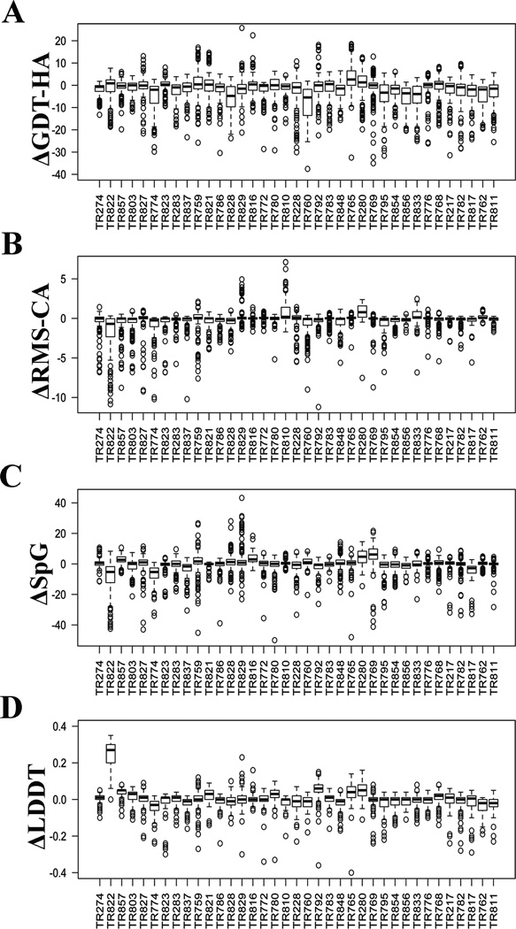
We first investigated the overall performance of the CASP predictors on the refinement targets before comparing the performance of individual groups against each other. Figure 1A shows box-and-whiskers plots of ΔGDT-HA (model – starting_structure) for each target over all the submitted models for each target (up to 5 per target per group). The targets are ordered by starting GDT-HA (lowest to highest, left to right), showing that there is no correlation of the distribution of ΔGDT-HA with the starting model quality. For 22 of 37 targets, the median ΔGDT-HA was negative, but for all of the targets, the maximum ΔGDT-HA was positive, indicating that at least one group was able to improve the starting model. The median and top values are also given in Table I.

Figure 1.

Summary of refinement of all the targets by different groups. Box and whiskers plots representing the relative change in A) ΔGDT-HA, B) ΔRMS-CA, C) ΔSpG, and D) ΔLDDT. The x-axis is sorted by the initial GDT-HA values (from lowest to highest, left to right).

Some of the targets were clearly easier than others for most groups. At least 60% of the groups significantly improved the quality of targets TR765, TR280, and TR823 (Table I). At least 50% of the predictors successfully refined an additional seven targets. Targets TR856 and TR762 proved most difficult with less than 10% of the predictors showing any refinement. The best examples include targets TR829, TR816, TR765, TR792, and TR759 where an improvement of more than 15 GDT-HA units was observed. However, in none of these examples is the best model the same as model 1. This suggests that despite performing good refinement the predictors have failed to identify the model closest to the native in these examples.

Since the RMSD metric is commonly used in structure refinement, we also calculated the distribution of the change in Cα RMSD (ΔRMS_CA) from the starting model to the refined model structures, where both are compared to the native structure (Figure 1B). In this case, a negative value of ΔRMS_CA reflects that the quality of the model has improved; the targets are ordered as in Figure 1A (by starting GDT-HA). The best examples with this metric include TR810, TR829, and TR816 which also have high ΔGDT-HA. While every target displays at least one favorable ΔGDT-HA, some targets have no favorable ΔRMS_CA scores. There were only two difficult targets (TR759 and TR829) that showed considerable refinement (by more than 2 Å RMS_CA) despite the high initial RMS_CA of more than 4 Å with the native. Overall no clear correlation was observed in the quality of the initial structures and the predicted models.

Local scoring metrics, which measure the accuracy of short atom-atom distances, are complementary measures to global metrics such as GDT-HA and RMSD. The distributions of SpG (SphereGrinder, Figure 1C) and LDDT (Local Distance Difference Test, Figure 1D) for each target, sorted by starting GDT-HA demonstrate that success in the global measures is not necessarily correlated with success in the local measures. For instance, TR828 has no significant improvement in GDT-HA but a number of models have significant increases in the SpG score (Figure 1C). Target TR822 had an unusually low value of starting LDDT (0.16) and almost all of the predictors managed to improve this value.

Using combination of metrics for assessment – TR829 example

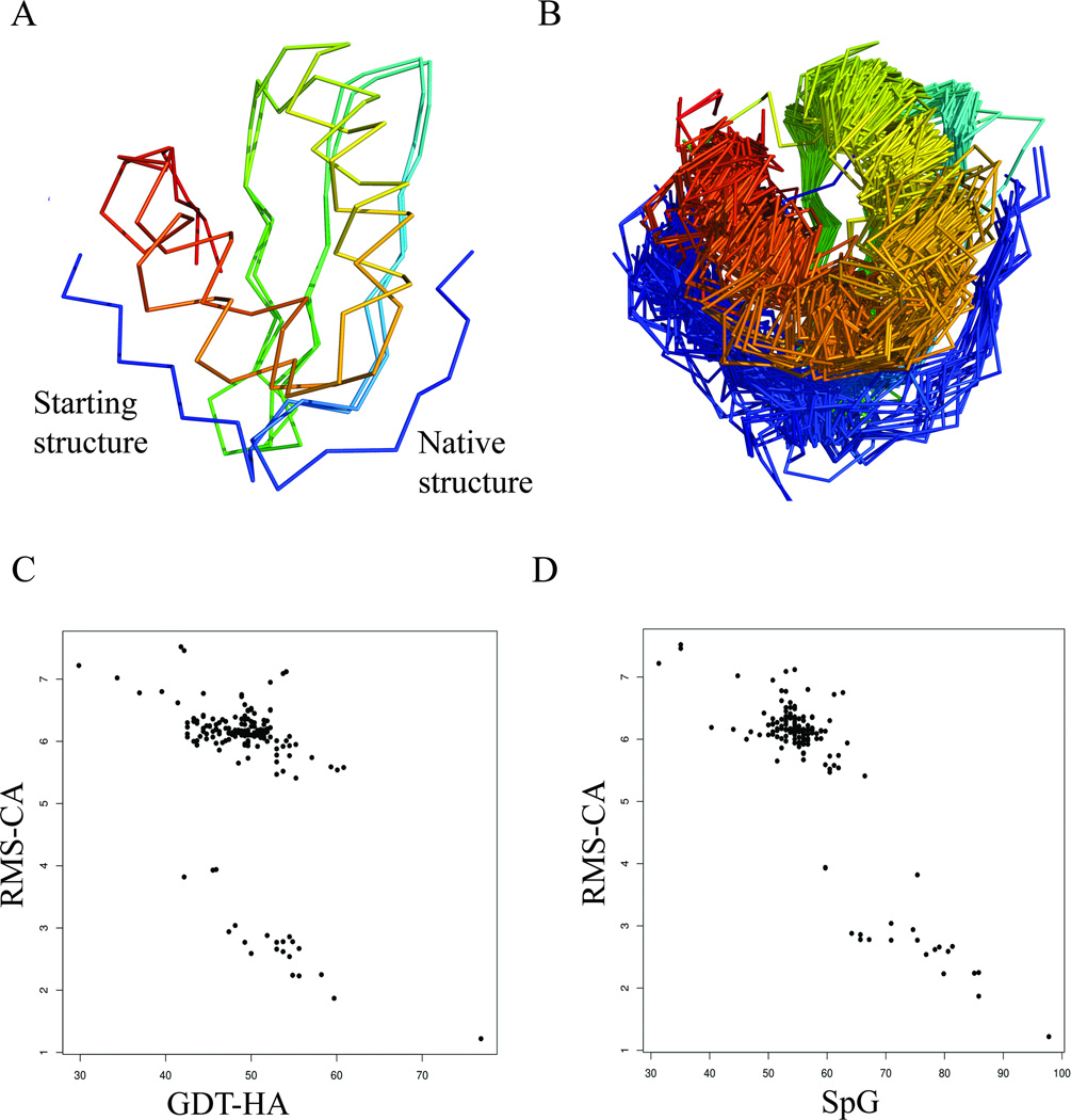
We investigated how the different metrics behave on a target with a defined change in structure between the starting structure and the experimental structure. For target TR829, the predictors were told that “The most problematic region is N-terminal residues 2–9.” The refinement of the starting structure of TR829 requires a repositioning of this N-terminal region from one side of the protein to the other (Figure 2A); 25 of 210 models included this movement (Figure 2B).

Figure 2.

Assessment of refinement in TR829. A) Superposition of initial and native structure. The main region to be refined is the N-terminus (residues 2–9). B) Superposition of the refined models for TR829. Some models were able to refine the position of the N-terminus successfully; C) Relationship between RMS_CA and GDT-HA for all models or TR829. Models with RMS_CA<4 Å successfully modeled the N-terminus; D) Relationship between RMS_CA and SpG for all the models of TR829.

We examined whether the various measures used in CASP were able to identify the models with the correctly positioned N-terminus. Intuitively, one model which correctly predicts this change would be expected to show a corresponding increase in GDT-HA and a decrease in RMS-CA. Surprisingly, we do not see the expected inverse relationship between RMS-CA and GDT-HA (Figure 2C). Visualization of the structures with low RMS-CA (<4 Å) showed that all of these refined structures had the N-terminus repositioned to form a short β sheet strand with strand 2 of the β sheet, while those with higher RMS-CA (all >5.4Å) retained the N-terminus adjacent to C-terminal helix. GDT-HA does not capture the difference between those structures with the correctly modeled N-terminus and those without. The trend is, however, clearly captured in relationship between RMS-CA and SpG values (Figure 2D). Although it is not clear why GDT-HA fails to reflect the N-terminus movement, this clearly demonstrates that a fair assessment of refinement benefits combination of different metrics. A similar phenomenon occurs for other targets where GDT-HA did not capture large-scale movements while RMSD and to some extent SpG did (Supplementary Fig. S1 and S2).

Refinement performance by top groups

The starting structures provided by CASP include proteins of different sizes and folds, and a successful refinement method should perform consistently over the majority of targets. An overall assessment of the refinement performance of the predictors can be gained by computing the percentage of their predicted models which were better than the starting structures. Table II provides a list of groups who have successfully improved the quality of the initial structures in at least 50% of the targets. The performance of five groups (FEIG, Seok-server, RFMQA, Kiharalab and PRINCETON_TIGRESS) exhibit improvement for >70% of the targets. There are eleven additional predictors who exhibit modest performance by successfully refining the starting structure to native-like for >50% of the targets. The remaining 37 groups worsened the structure for the majority of targets (data not shown).

Table II.

Performance of top groups in CASP11 refinement

	Group	Targets Submitted	Successful Predictions	Percentage
1	FEIG	37	29	78.37
2	Seok-server	37	29	78.37
3	RFMQA	35	27	77.14
4	Kiharalab	37	27	72.97
5	PRINCETON_TIGRESS	37	27	72.97
6	Seok	37	25	67.56
7	LEER	35	22	62.85
8	Seok-refine	37	23	62.16
9	KnowMIN_server	37	23	62.16
10	LEE	37	22	59.45
11	Schroderlab	37	21	56.75
12	PRINCETON_MD_REFINE	37	20	54.05
13	MULTICOM-CONSTRUCT	37	20	54.05
14	Bates_BMM	34	18	52.94
15	BAKER-REFINESERVER	36	19	52.77
16	nns	37	19	51.35

The table reports values only for those groups who submitted models for at least 19 of 37 targets, and have improved the starting structure of at least 50% of the targets for model 1.

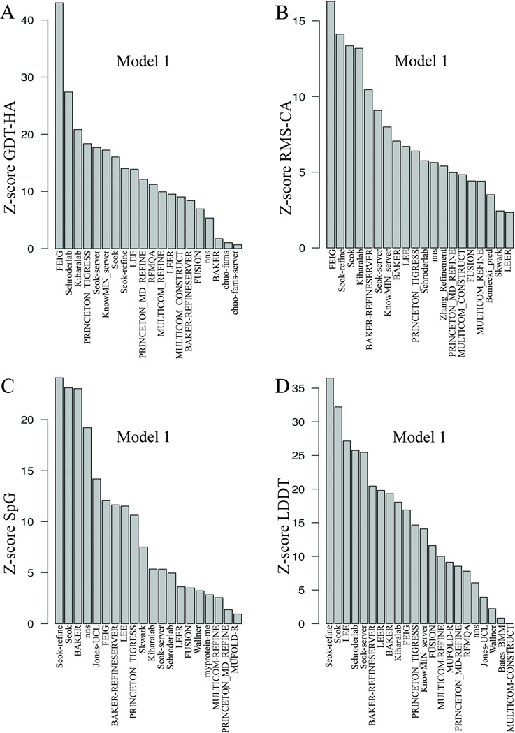
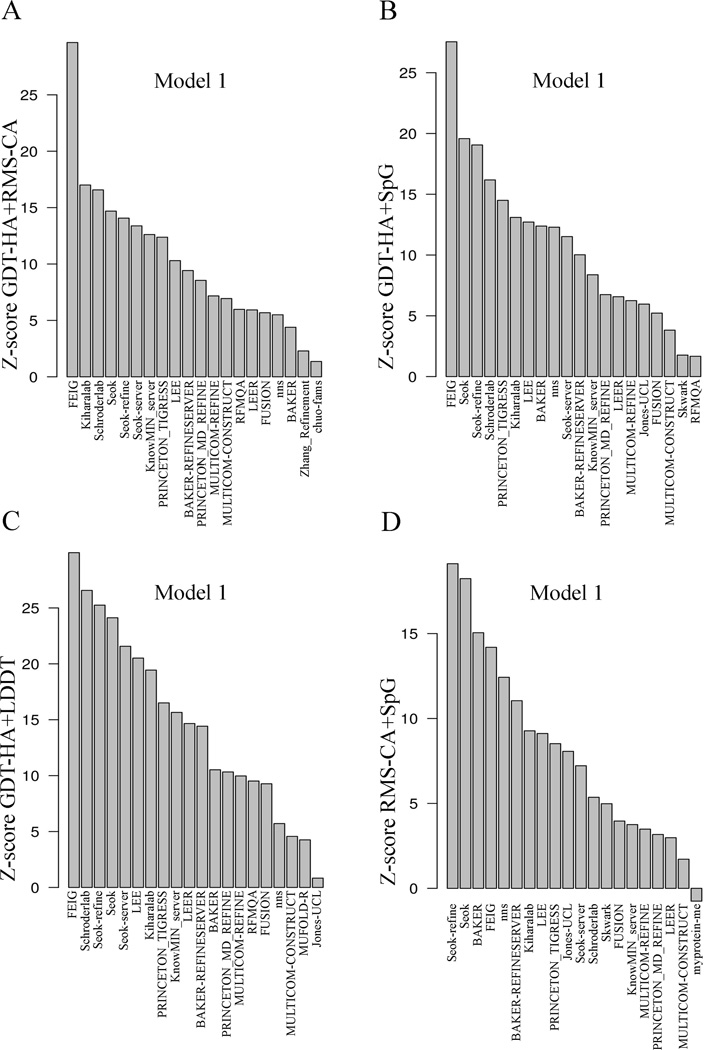
To evaluate the performance of the predictor groups, we first utilized the standard CASP metrics, singly, pairwise, and in various combinations. To combine multiple measures of performance, the Structure Prediction Center provides data in the form of Z-scores for each measure and a tool for summing various combinations of measures. We used this tool to calculate the ranks of the predictor groups for single measures, pairs of measures, and combinations of measures. The Z-scores based on single, pairwise, and multiple-summed metrics calculated for the model 1 of the top twenty groups are shown in Figure 3, 4 and 5 respectively. The Feig group achieved the best summed Z-score of GDT-HA (Figure 3A), Z-score of RMS-CA (Figure 3B), Z-score of GDT-HA+RMS-CA (Figure 4A), and Z-score of GDT-HA+SpG (Figure 4B). The other top predictors, Seok, Seok-refine, Schroderlab, Kiharalab, and PRINCETON_TIGRESS also performed consistently. FEIG performs less well on the local measures, SpG (Figure 3C) and LDDT (Figure 3D), when considered singly. These measures emphasize side-chain packing and other close atomic contacts. For these measures, Seok-refine, Seok, and BAKER end up on top. While the Z-score sums that included GDT-HA decreased rapidly after the first group, the Z-score(RMS-CA) and Z-score(SpG) remained high for the first 4–5 groups.

Figure 3.

Summary of Z-scores for single metrics of model 1 of top 20 groups. The x-axis in all the plots displays the group names. The y-axis is the Z-score for each single metric: A) GDT-HA; B) RMS-CA; C) SpG; D) LDDT

Figure 4.

Summary of Z-scores for pairwise sums of metrics of model 1 of top 20 groups. The x-axis in all the plots displays the group names. The y-axis is the Z-score for pairs of metrics: A) GDT-HA+RMS-CA, B) GDT-HA+SpG C) GDT-HA+LDDT, D) RMS-CA+SpG

Figure 5.

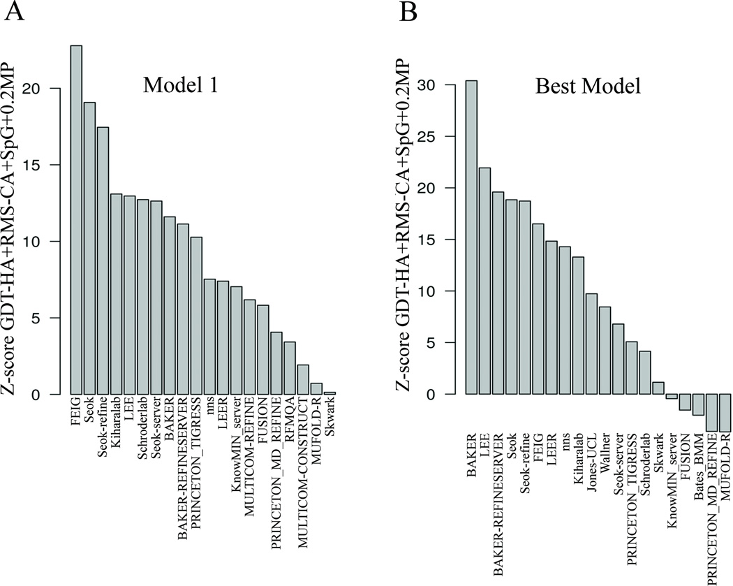
Summary of sum of Z-scores of metrics for model 1 and best models of top 20 groups. The x-axis in all the plots displays the group names. The y-axis is the sum of Z-scores for GDT-HA+RMS-CA+SpG+0.2MP computed for A) Model 1 and, B) Best models.

Molprobity reflects whether the predicted structure has few atomic clashes and backbone and side-chain conformations consistent with statistical analyses of the PDB. While not a reflection of similarity to native, good MolProbity scores (MP scores) indicate that the predicted structure would easily serve as a good starting model for MD simulations or refinement by other programs, and is therefore a desirable property in a refined model structure. We have combined it with the other measures to calculate a total Z-score for each model by summing {GDT-HA + RMS-CA + SpG + 0.2MP} (Figure 5A). The scaling of MP score by 0.2 is somewhat arbitrary but was chosen to be the same as the value we used in the TBM assessment. It reflects that the range of Z-scores for MolProbity is much larger than the Z-scores for the other measures, and so prevents the MP score from overwhelming the measures which compare the models to the native structures.

The combined measure is an assessment of predictor performance that utilizes both local and global metrics with an emphasis on native-like backbone conformation. In this analysis (Figure 5A), FEIG performed best, followed closely by Seok and Seok-refine. By analyzing single metrics and combinations of different metrics, we get an overall picture of the same groups performing consistently though the rankings change among them. The analysis also highlights that the algorithms used by different predictors exhibit different abilities in model refinement. While Seok, BAKER, nns were better in short-range packing as assessed by local scoring metrics, FEIG, Schroder, and Kiharalab exhibit sustained improvement in backbone refinement.

Group performance based on Z-scores of the best models

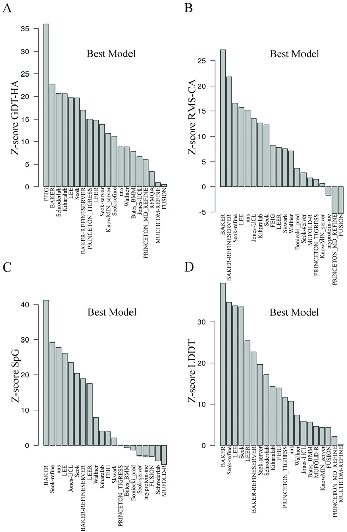
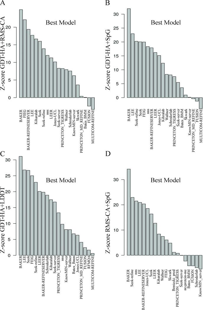
The Z-scores calculated from the best models submitted by each group for each target can highlight if any groups made good predictions but failed to identity them as model 1. As with model 1, we have calculated the summed Z-scores for each group for each individual measure (Figure 6), pairs of measures (Figure 7), and the summed Z-score (Figure 5B). The overall Z-score values for best models are generally higher than the values for model 1, indicating that most of the groups do not consistently submit their best model as model 1. The Z-score for the single metric, GDT-HA, for best models shows FEIG as the top performer by a significant margin (Figure 6A). The other top groups include BAKER, Schroderlab, Kiharalab, and LEE. The Baker group has moved from 17th place considering only model 1 (Figure 3A) to second place when considering the best models (Figure 6A). The same is also observed in Z-score of RMS_CA (Figure 6B) and Z-score of GDT-HA+RMS_CA (Figure 7A) where BAKER and BAKER-REFINESERVER emerged as the top predictors. nns and Jones_UCL were also among the top groups using these metrics. The Z-score for SpG (Figure 6C) and the sum of GDT-HA and SpG (Figure 7B) display similar trends with BAKER outperforming other groups followed by Seok-refine, nns and LEE. Therefore, the assessment based on the summed Z-score, {GDT-HA + RMS-CA + SpG + 0.2MP} (Figure 5B), for the best models is quite different from the assessment of model 1 (Figure 5A). It shows BAKER, LEE and BAKER-REFINESERVER as the top three groups. This clearly highlights that these groups are able to make good predictions but they do not consistently submit them as model 1. Three groups Seok, Seok-refine, and LEE always show high scores whether they are assessed by model 1 or their best models. FEIG, which performed the best in the model 1 analyses, falls to sixth position when the best models are assessed. This concern about limitations in recognizing the model closest to native as model 1 by different groups has also been expressed in previous CASP experiments.

Figure 6.

Summary of Z-scores single metrics of best models of top 20 groups. The x-axis in all the plots displays the group names. The y-axis is the Z-score for each single metric: A) GDT-HA, B) RMS-CA, C) SpG, D) LDDT

Figure 7.

Summary of Z-scores pairs of metrics of best models of top 20 groups. The x-axis in all the plots displays the group names. The y-axis is the Z-score for pairs of metrics: A) GDT-HA+RMS-CA; B) GDT-HA+SpG; C) GDT-HA+LDDT; D) RMS-CA+SpG.

Group performance based on relative scores

The Z-scores for refinement assess the performance of groups with respect to the predictions of all the other groups without regard to the starting structure provided by the CASP organizers. A positive Z-score only means that the structure is better than the mean prediction but it can still be worse than the initial structure. In addition, the range of each Z-score does not correlate with the range of improvements made to the models; even targets for which even the best models made modest improvements in the starting models will count as much as targets for which much larger improvements were made. An objective evaluation of the performance of predictors therefore also requires investigation into how different groups have improved the structure with respect to the initial structure. In order to do so we have calculated relative scores which reflect the improvement in the quality of the prediction with respect to the starting structure as described in the methods section. The summed relative score is the average percentage increase (calculated as a geometric mean and so a proper average of a ratio²⁵) in a score such as GDT-HA multiplied by the number of targets submitted by the group (see Methods).

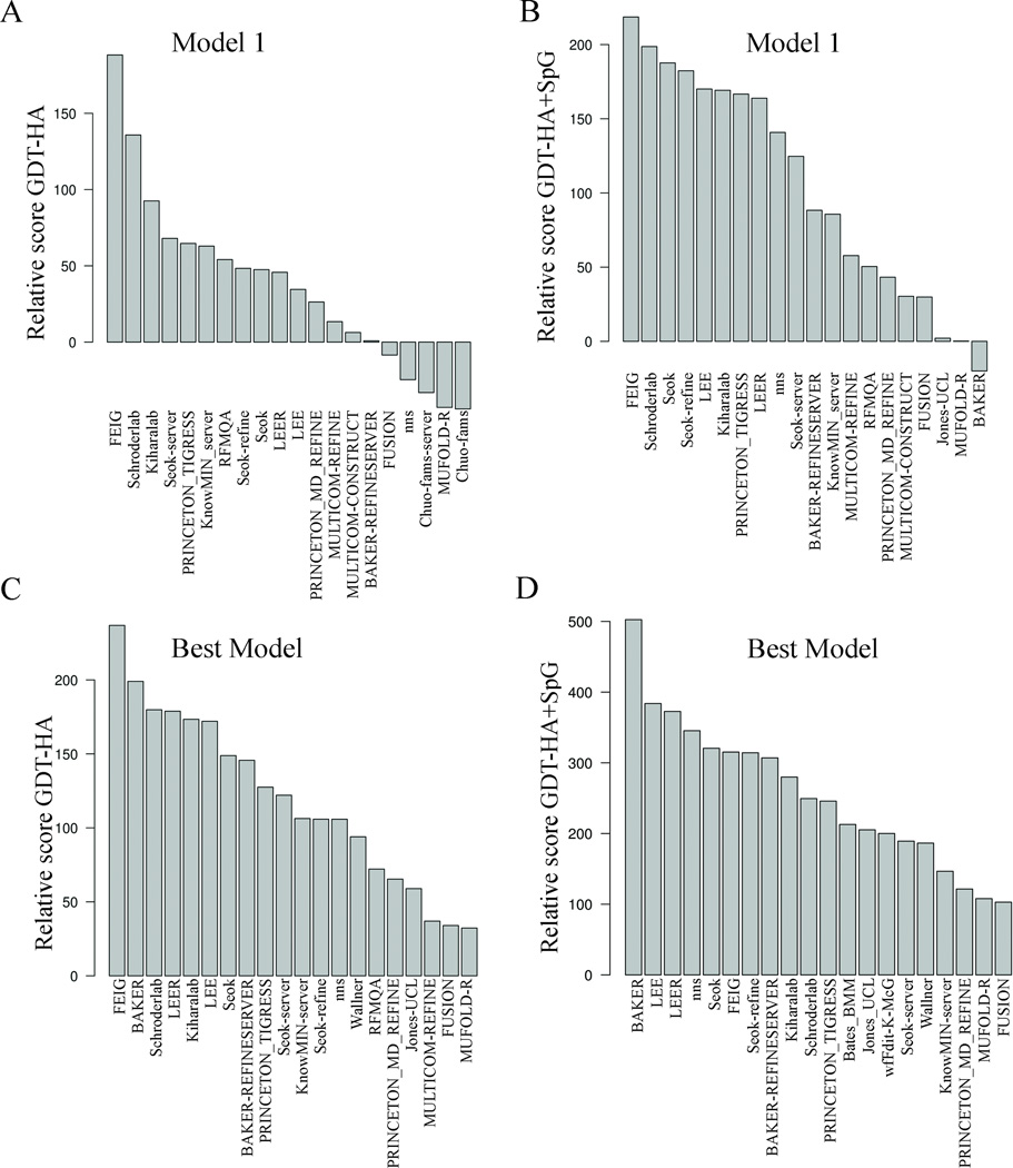
The summed relative GDT-HA scores calculated for model 1 is positive for 15 predictors out of 37, showing that less than half of the predictors have refined the starting structures on average (Figure 8A). The groups FEIG, Schroderlab, and Kiharalab are the top predictors considering only relative improvements in GDT-HA. The sum of relative scores for {GDT-HA+SpG} produces FEIG, Schroderlab, Seok, and Seok-refine as the top groups (Figure 8B), although with a smaller difference between the top groups than for GDT-HA alone (Figure 8A). Not surprisingly, the assessment of top groups by regular Z-scores or by relative scores has highlighted the same predictors. Moreover, like the Z-scores, we observe that the relative GDT-HA score of the top groups falls rapidly indicating that sustained backbone improvement across all targets is difficult even for the best groups. However, consistently high scores are observed for the combined GDT-HA and SpG relative metric, showing that most of the groups perform better in improvement of local packing.

Figure 8.

Summary of relative scores of top 20 groups. The x-axis in all the plots displays the group names. The y-axis is the relative score for different metrics: A) GDT-HA for model 1; B) GDT-HA+SpG for model 1; C) GDT-HA for best model; D) GDT-HA+SpG for best model. The scores are calculated only for the groups who have predicted at least 35 out of 37 targets.

The relative score GDT-HA computed from best models of all the groups shows that FEIG, BAKER, Schroderlab, LEER, Kiharalab, and LEE perform well (Figure 8C), while BAKER, LEE, LEER, and nns are the best scores for the sum of relative GDT-HA+SpG scores (Figure 8D). Similar observations were made for Z-scores of the same metrics (Figure 7B) for the top groups. BAKER produces the best refinements but does not identify the best models as model 1.

Distribution of relative refinement score of top groups

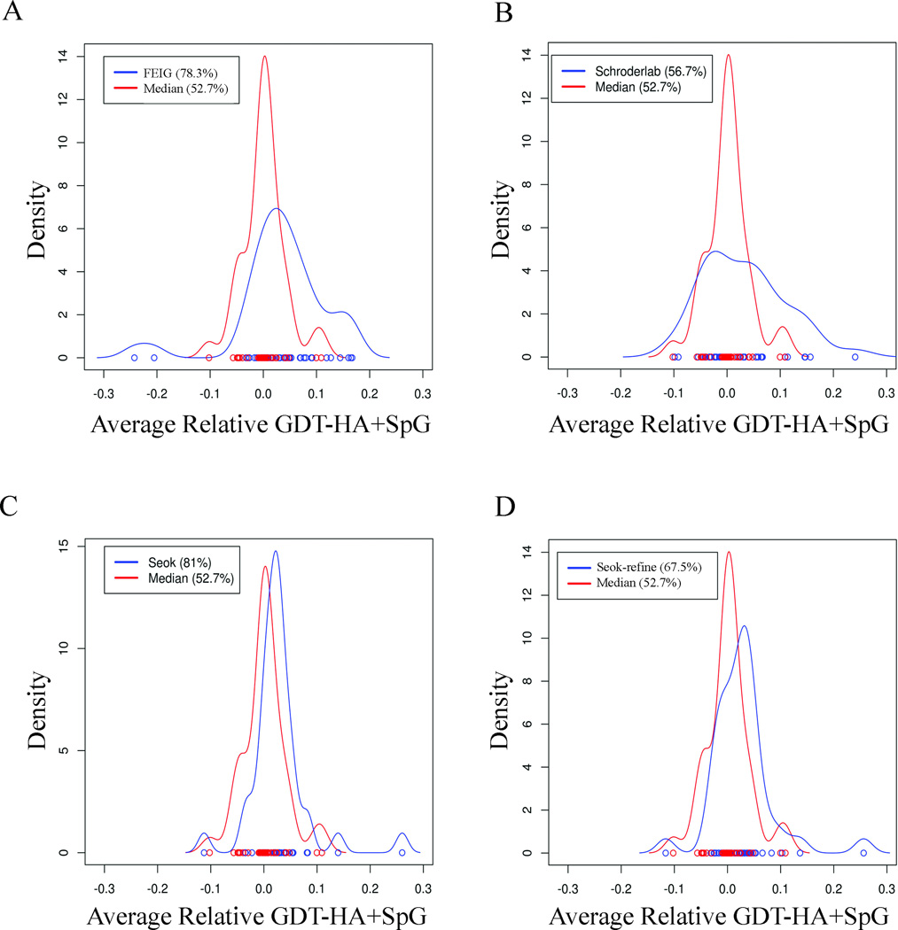
It is useful to compare the distribution of relative scores for each group across the targets and to compare these distributions with each other and with the “median group.” We chose a median group as one with the lowest positive summed relative score. This group ranks 16 out of 30 groups that had submitted at least 35 targets. Figure 9 shows the distribution of the relative scores (sum of GDT-HA and SpG) of the top groups compared with the median group. FEIG improved 78% of their models better than the starting structures as compared to 53% for the median group (Figure 9A). The second group, Schroderlab, improved 57% of models (Figure 9B). Although Schroderlab improved fewer total targets, some of its refinements were quite successful. The third group, Seok had positive scores for the largest number of targets (81%) (Figure 9C) but with moderate performance on each. Seok-refine behaves more like Schroderlab with relatively moderate performance in the number of targets improved (67.5%) but producing a few refinements with higher scores (Figure 9D).

Figure 9.

Kernel density plots comparing the relative scores of top groups with the median group. The median group here is referred to the group which has least positive relative score. A) FEIG; B) Schroderlab; C) Seok; D) Seok-refine. The scores are calculated only for model 1. The numbers in parenthesis are the percentage of targets with score greater than 0.

Comparison of quality of all five models submitted by top groups

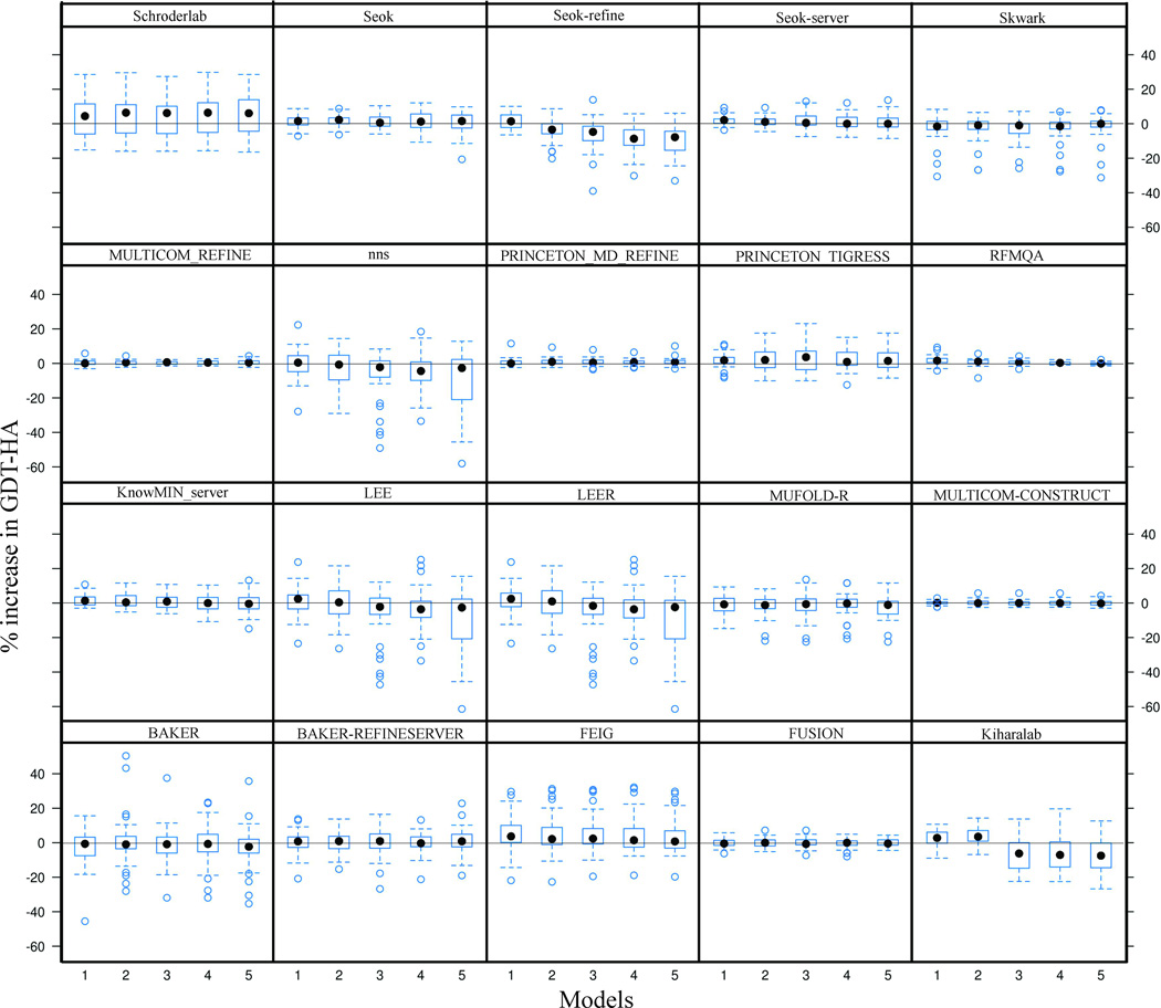
The comparison of model 1 predictions with the best models for each group showed that many groups do not identify the best model as model 1. This concern has also been expressed in previous CASP assessments. We have systematically compared the percent increase in GDT-HA of each of the five models submitted by the top groups (Figure 10). The figure shows that for groups like Seok-refine, Kiharalab, and FEIG the mean GDT-HA decreases from model 1 through model 5, consistently identifying the prediction closest to native as model 1. This difference in mean GDT-HA between different models is also observed in predictions from groups like LEE and LEER. Although the mean GDT-HA of their model 1 is higher than the others but they fail to identify some of the best models which are submitted as model 4. On the other hand, groups like Seok and Schroderlab have the mean values of all the predictions close to each other and there is only small variation in the distributions by model number. The sharpest discrepancy is observed for the Baker group where the predictions with highest GDT-HA are not submitted as model 1 but are distributed across models 2, 3, 4, and 5.

Figure 10.

Lattice plot displaying percent change in ΔGDT-HA for models 1–5 of top twenty groups.

Contact heat maps as a tool for identifying regions of refinement

The numerical analysis provides an overall idea of the refinement success of the different groups. But we were also interested in what kinds of improvements in the structures were made, particularly the question of whether positive scores were due to observable improvements in large loops or in the positions of secondary structures relative to each other, or whether positive scores were due to smaller changes across the model structure. To examine this, we developed a form of heat map to identify changes in Cα-Cβ distances in the starting structure that bring the model closer to (or further away from) the target structure. By marking the secondary structure along the chain sequence on each axis we can observe whether the motions involved particular elements of secondary structure, the loops between them, or the positions of the N and C terminal segments in a manner independent of structure superposition. In this section we discuss the refinement of six representative examples to illustrate the success and limitations of different prediction groups with heat maps (Figure 11, 12, and 13). The color range in each figure is the same, so that the extent of optimization of distances can be compared. To supplement this, Table III provides comparative analysis of percent increase in GDT-HA for model 1 of all the targets submitted by the top six groups. Where the heat maps identified specific changes in structure, such as the motion of helices or the formation of β sheet strands at the N or C terminus that were missing in the starting structure, these are noted in Table III.

Figure 11.

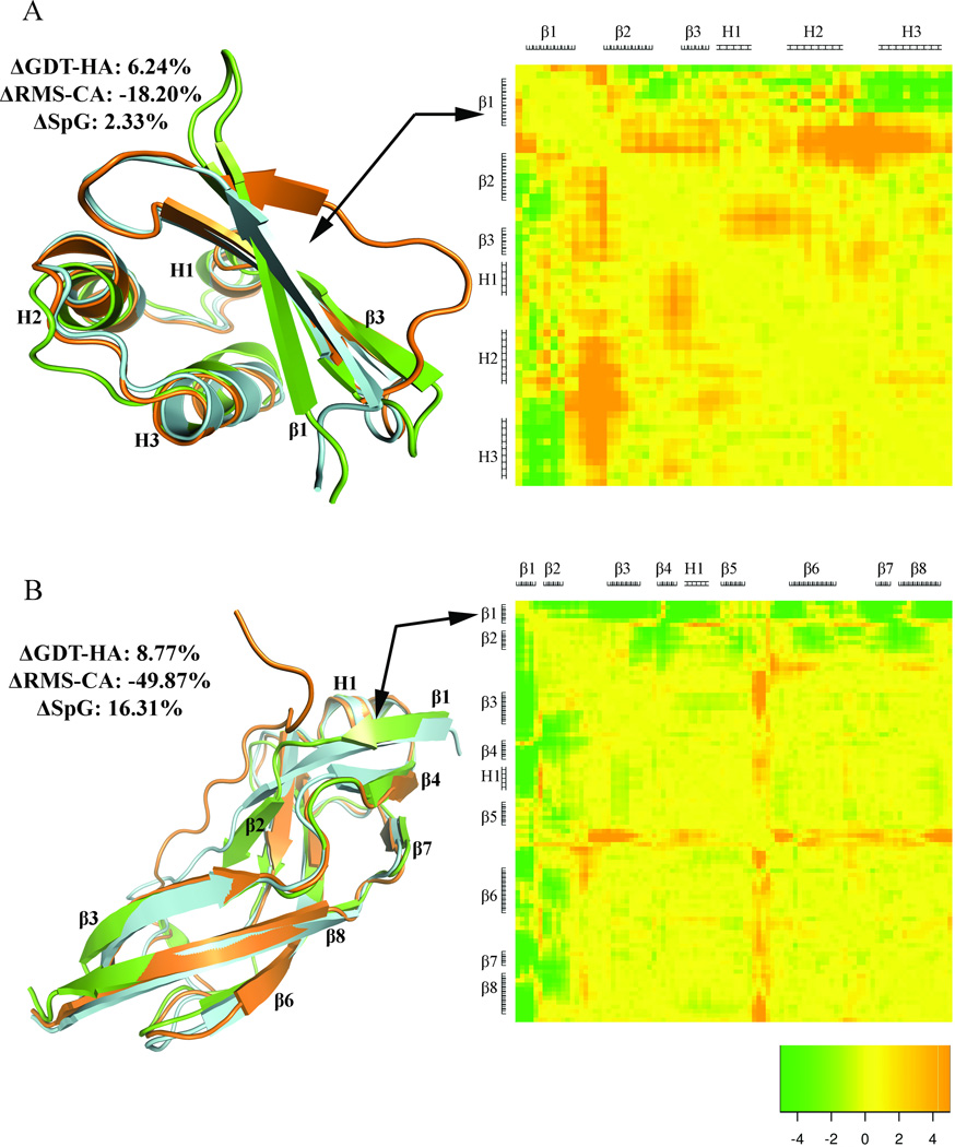
Refinement of internal helices. The successful refinement of helices is displayed in molecular plots and heat maps for A) TR765, model 1 (FEIG) and B) TR821, model 1 (Schroderlab). The starting structure, target and model are displayed in orange, green and cyan colors respectively. The numbers represent percent increase in ΔGDT-HA, ΔRMS-CA and ΔSpG. The secondary structural regions of the target as helices (H) and sheets (E) are represented along each axis of the heat map. A negative value (green color) displays more native-like atom-atom distances and a positive value (orange color) displays less native-like distances.

Figure 12.

Refinement of N-terminal strand. The successful refinement of N-terminal strands is displayed in molecular plots and heat maps for A) TR759, model 1 (Seok-refine) and B) TR280, model 1 (LEE). The starting structure, target and model are displayed in orange, green and cyan colors respectively. The numbers represent percent increase in ΔGDT-HA, ΔRMS-CA and ΔSpG. The secondary structural regions of the target as helices (H) and sheets (E) are represented along each axis of the heat map. A negative value (green color) displays more native-like atom-atom distances and a positive value (orange color) displays less native-like distances.

Figure 13.

Refinement of C-terminal loop segment and a β-sheet. The successful refinement of C-terminal loop segment and β-sheet is displayed in molecular plots and heat maps for A) TR833, model 1 (Seok-refine) and B) TR822, model 1 (LEE). The starting structure, target and model are displayed in orange, green and cyan colors respectively. The numbers represent percent increase in ΔGDT-HA, ΔRMS-CA and ΔSpG. The secondary structural regions of the target as helices (H) and sheets (E) are represented along each axis of the heat map. A negative value (green color) displays more native-like atom-atom distances and a positive value (orange color) displays less native-like distances.

Table III.

Percent increase in GDT-HA of model 1 of all targets refined by top six groups.

Targets	FEIG	Seok	Seok-refine	Kiharalab	LEE	Schroderlab
TR217	0.18	2.19	−3.11	−2.56	−3.83	−7.49
TR228	1.59	6.41	3.73	−4.29	−3.75	7.47 Helices
TR274	−1.40	−4.22	−3.29	−6.11	3.74	−11.27
TR280	10.98 Nter moved	8.77 Nter moved	7.46 Nter strand	2.20	8.77 Nter strand	20.19 Nter moved
TR283	0.02	2.34	2.73	6.21	0.41	−3.09
TR759	24.11	−2.67 Nter strand	6.24 Nter strand	10.71	2.67	16.96 Sheet
TR760	0.43	3.24	0	1.94	−7.53	−10.98
TR762	−6.18	−1.65	−6.45	−2.61	−1.79	−10.85
TR765	29.66 Helices	0.54	1.10	10.44	9.34	28.56 Helices
TR768	8.10	2.96	5.13	2.42	12.15	7.01
TR769	1.72	−0.45	−0.01	9.03	0.85	10.76
TR772	2.39	−0.70	0.72	−1.67	−0.22	−5.02
TR774	5.54	−5.08	−5.08	0.45	−0.84	−6.79
TR776	8.35	0.71	0.17	5.50	3.54	4.43
TR780	8.22	6.77	5.80	6.29	11.60	9.19
TR782	12.89	1.39	−1.39	2.79	3.47	11.49
TR783	8.51	1.77	1.41	4.44	2.49	6.39
TR786	7.74	−1.18	−5.39	−4.70	4.68	10.33
TR792	27.57 Helices	−2.16	−2.16	−0.53	0	14.06
TR795	8.57	4.90	3.67	6.12	2.45	6.74
TR803	11.94	0	4.34	4.34	7.60	−6.00
TR810	2.00	4.82	8.04	2.81	−3.41	4.42
TR811	−6.24	2.16	2.43	−0.27	6.23	−8.40
TR816	7.79	3.53	1.40	3.54	3.54	16.31 Helix & Loop
TR817	−14.36	1.56	−3.84	0.28	−9.95	−4.97
TR821	23.60 Helices	3.59	6.18	7.99	−4.20	28.39 Helices
TR822	23.75 Sheets	2.88	10.07	8.66	23.75 Sheets	19.45 Sheets
TR823	−21.8	5.88	2.51	8.61	2.92	14.49
TR827	3.32	3.32	8.08	3.69	14.33	18.39
TR828	−4.75	−7.09	−4.75	1.76	−10.05	−9.48
TR829	1.46	−5.84	−2.19	3.63	2.19	−2.93
TR833	2.23	1.10	4.07 C-ter refined	3.34	−23.41	−5.95
TR837	−3.31	2.83	6.59	2.37	7.07	−1.41
TR848	3.68	−2.46	−3.39	−8.93	−0.30	10.15
TR854	10.03	0.59	−5.93	0.57	−12.42	−0.59
TR856	−1.01	1.52	0.25	−0.49	−8.57	−15.14
TR857	10.66	7.62	6.82	8.38	3.78	3.78

Where significant improvements in elements of secondary structure were observed in the heat maps, this is notated below the score. For target TR822, the starting structure did not contain a proper β sheet, while several groups were able to create one during refinement.

The refinement of helices in the interior of the protein sequence (i.e. those not at the N or C terminus) is a difficult task as they are restrained by surrounding structural elements. FEIG and Schroderlab have successfully done such refinement for targets TR765 and TR821 displayed in Figure 11A and 11B respectively. FEIG’s refinement exhibits displacement of the helix H1 in the structure with respect to other secondary structural elements subsequently forming more native-like Cα-Cβ contacts. This can be seen on the heat map in the region corresponding to helix H1 dominated by green color, showing motion of H1 towards a more native-like position relative to β1, β2, β3, H2 (at least the C-terminal half of H1 is better positioned), and β4. However, the overall refinement is limited by the non-native like orientation of the loop between the β-strand β1 and helix H1 in the structure. The heat map is predominantly orange in color in this region owing to Cα-Cβ distances more unlike the native than the starting structure. The refinement of TR821 by Schroderlab includes at least four helices in the interior of the protein (Figure 11B). The helices move outwards from the core and as a result there is improved helix-helix packing. The refinement is most clear in the region extending from helix H7 to end of helix H10 which is reflected in the heat map in mostly green color displaying native like contacts of these helices with other parts of the protein. Moreover, the loop between helix H10 and H11 is also better positioned as is clearly seen both in the superposition and the heat map.

Figures 12A (TR759) and 12B (TR280) represent successful refinement of N-terminal strand of targets TR759 and TR280 by the groups Seok-refine and LEE respectively. In the starting structure of both of these examples, the N-terminus is in a coil-like conformation away from the position in the experimental structure. The refinement by both groups not only moves the N-terminus closer to native but also correctly generates the β1 strand. However, in TR759 (Figure 12A) the exact alignment of β1 with respect to the other regions of the protein could not be completely achieved. But since it moves towards the helix H3 which is close to a native-like orientation, the region corresponding β1 and helix H3 is seen as green in the heat map. However, the loop between β1 and β2 does not move and is observed in orange color in the heat map with respect to other regions of the protein. On the other hand, in TR280 all the other regions except the N-terminus β1 in the starting structure are already close to native. The movement of β1 in the refined position aligns it correctly with other regions of the protein seen in the heat map as almost entirely green.

Figures 13A shows an example of the refinement of C-terminal coil region of TR833, which is far from the native orientation in the starting structure. The refinement successfully predicts the native like conformation and moves the C-terminal closer with respect to the β-sheets of the protein. This refinement of the C-terminus by aligning it correctly with respect to the entire protein is clearly observed in the heat map as the long green strip. Conversely, Figure 13B shows a more global refinement of another target, TR822, by LEE. The starting structure of TR822 does not have clearly defined β-sheets, and the presence of a large number of loops makes it a relatively difficult target to refine. The structure was significantly refined by LEE who successfully generates the fourth, fifth, and sixth strands (β8, β11 and β13) of the second β sheet. This is seen as green in the heat map. However, since the loop regions of the structure are not refined to native-like orientation the green color is interspersed with yellow/orange.

Comparison to CASP10

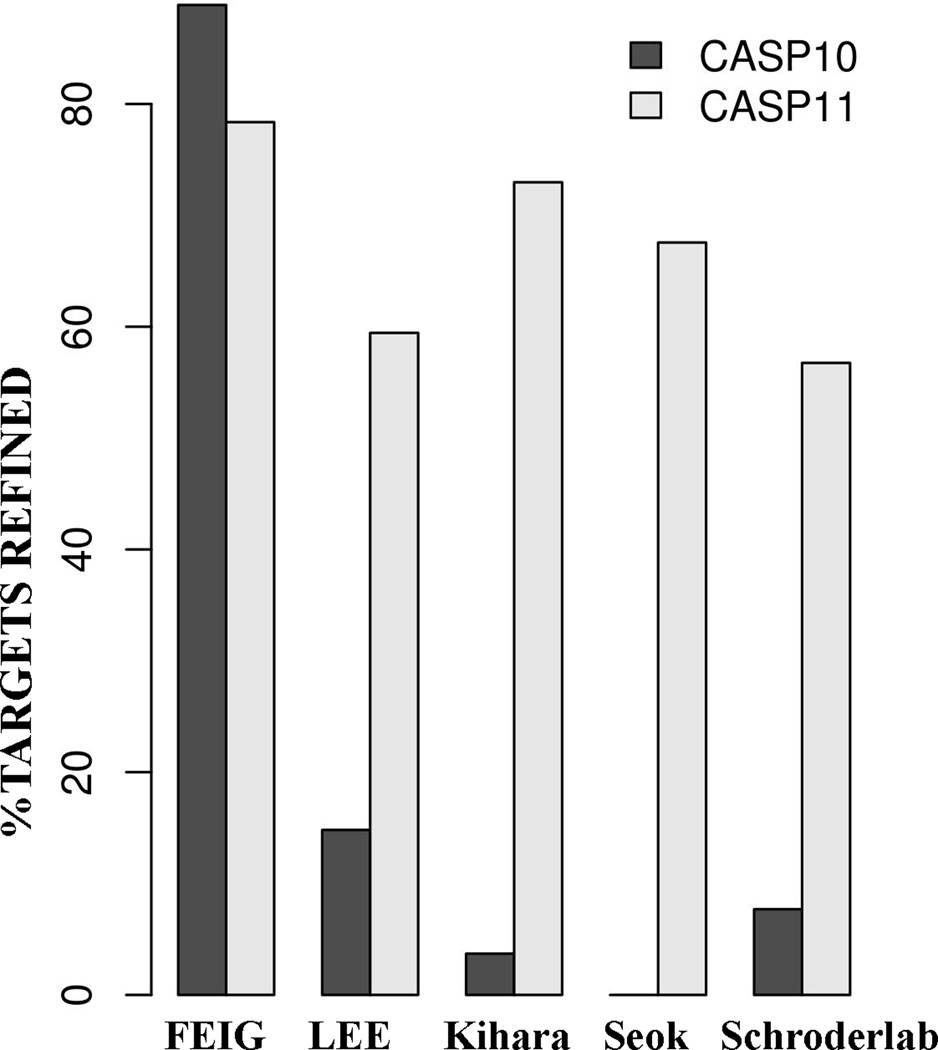
The refinement of template-based models has proved to be a difficult task since its introduction in CASP8. The predictors have struggled to exhibit consistent refinement across the different targets. However, in CASP10 FEIG’s molecular dynamics based method successfully refined most of the 27 targets. The number of targets has been increased to 37 in CASP11. But the lack of a good measure of target difficulty limits a direct comparison of the performance of different groups in CASP11 with the previous years. However, despite this limitation computing the percentage of targets refined provides an overall picture of the progress in the field. Figure 14 compares the performance of some of the top groups in CASP11 with their predictions in CASP10. FEIG is consistent in its performance by refining ~80% of the targets successfully in both CASP10 and CASP11. In CASP11, four other groups were able to improve on their CASP10 performance substantially, including LEE, Kihara (different group name in CASP10), Seok, and Schroderlab.

Figure 14.

Comparison of the performance of top groups in CASP11 with CASP10. The percentage of targets refined successfully is displayed. A target is assumed to be refined if the GDT-HA of submitted model is more than the starting structure. Only model 1 is considered for this analysis. The total numbers of targets were 27 and 37 in CASP10 and CASP11, respectively.

Discussion

We have assessed the performance of 53 groups in the refinement task in CASP11 using the standard Z-scores provided by the Structure Prediction Center and also relative scoring measures that summarize the percent improvement in GDT-HA and SpG scores over the starting structures. We showed that different individual measures ranked the groups in different orders, and in particular global measures such as GDT-HA and RMS_CA are distinct from local measures such as SpG and LDDT. As with the CASP10 assessment,¹⁷ in a summary measure consisting of {GDT-HA+RMS_CA+SpG+0.2MP} we weighted improvements in backbone conformation more highly than local measures assessing atom-atom packing.

By calculating relative scores, we were able to quantify sustained levels of improvements in the starting structures by some of the groups. With this score, we found that the top groups were able to improve GDT-HA scores by 5.1% (FEIG), 3.7% (Schroderlab), and 2.5% (Kiharalab). Similarly, GDT-HA+SpG taken together was improved by 5.9% (FEIG), 5.4% (Schroderlab), and 5.1% (Seok).

Finally, we introduced a visualization of refinement by means of a heat map that shows where Cα-Cβ distances between different regions of the protein were made more native-like (successful refinement) or non-native like (unsuccessful or no refinement) than those in the starting structure. This enabled us to describe the improvements in the structure in terms of the relative placement of secondary structure units at the N and C termini or interior to the protein. The most common significant changes were in the placement of the terminal segments, whether coil or β strands that were misplaced in the starting structure. In only a few cases could we identify significant improvements in internal helices, and for one target we found improvements in several internal β strands because the starting structure contained strand segments that were not close together enough to be identified as a β sheet. This method of visualization and quantification that can be derived from it may enable developed to focus their efforts on specific aspects of refinement that are the most challenging (e.g., the positions of internal units of secondary structure).

We evaluated whether the top groups in the CASP11 assessment improved upon their results in CASP10. The FEIG group maintained the same high rate of success, ranking first in both CASP10 and CASP11, by refining approximately 80% of the targets in both experiments. But other groups are now able to refine significantly more than half of the targets, ranging from 60 to 75% of the targets, while in CASP10 the same groups succeeded for less than 20% of the targets.

The top groups in CASP11 used a variety of methods for refinement: variations of molecular dynamics methods (FEIG, Schroderlab, and LEE), alternating side-chain repacking and MD simulations (Kihara), and hybrid knowledge-based and molecular mechanics energy functions (Seok). Although the improvement in the quality of the models refined by these groups is modest is most cases but the success of different kinds of approaches is promising progress in CASP11. The future experiments will show if any method has any specific advantage over others.

References

- 1.Moult J. A decade of CASP: progress, bottlenecks and prognosis in protein structure prediction. Curr Opin Struct Biol. 2005;15:285–289. doi: 10.1016/j.sbi.2005.05.011. [DOI] [PubMed] [Google Scholar]
- 2.Kryshtafovych A, Fidelis K, Moult J. CASP10 results compared to those of previous CASP experiments. Proteins: Structure, Function, and Bioinformatics. 2014;82:164–174. doi: 10.1002/prot.24448. [DOI] [PMC free article] [PubMed] [Google Scholar]
- 3.Baker D, Sali A. Protein structure prediction and structural genomics. Science. 2001;294:93–96. doi: 10.1126/science.1065659. [DOI] [PubMed] [Google Scholar]
- 4.Anishchenko I, Kundrotas PJ, Tuzikov AV, Vakser IA. Structural templates for comparative protein docking. Proteins. 2015;83:1563–1570. doi: 10.1002/prot.24736. [DOI] [PMC free article] [PubMed] [Google Scholar]
- 5.Kaufmann KW, Meiler J. Using RosettaLigand for small molecule docking into comparative models. PLOS ONE. 2012;7:e50769. doi: 10.1371/journal.pone.0050769. [DOI] [PMC free article] [PubMed] [Google Scholar]
- 6.Bordogna A, Pandini A, Bonati L. Predicting the accuracy of protein-ligand docking on homology models. J Comput Chem. 2011;32:81–98. doi: 10.1002/jcc.21601. [DOI] [PMC free article] [PubMed] [Google Scholar]
- 7.Fan H, Irwin JJ, Webb BM, Klebe G, Shoichet BK, Sali A. Molecular docking screens using comparative models of proteins. Journal of chemical information and modeling. 2009;49:2512–2527. doi: 10.1021/ci9003706. [DOI] [PMC free article] [PubMed] [Google Scholar]
- 8.Yue P, Li Z, Moult J. Loss of protein structure stability as a major causative factor in monogenic disease. J Mol Biol. 2005;353:459–473. doi: 10.1016/j.jmb.2005.08.020. [DOI] [PubMed] [Google Scholar]
- 9.Zhang Y. Interplay of I-TASSER and QUARK for template-based and ab initio protein structure prediction in CASP10. Proteins: Structure, Function, and Bioinformatics. 2014;82:175–187. doi: 10.1002/prot.24341. [DOI] [PMC free article] [PubMed] [Google Scholar]
- 10.Joo K, Lee J, Sim S, Lee SY, Lee K, Heo S, Lee IH, Lee SJ, Lee J. Protein structure modeling for CASP10 by multiple layers of global optimization. Proteins. 2014;82(Suppl 2):188–195. doi: 10.1002/prot.24397. [DOI] [PubMed] [Google Scholar]
- 11.MacKerell AD, Bashford D, Bellott M, Dunbrack RL, Evanseck JD, Field MJ, Fischer S, Gao J, Guo H, Ha S, Joseph-McCarthy D, Kuchnir L, Kuczera K, Lau FT, Mattos C, Michnick S, Ngo T, Nguyen DT, Prodhom B, Reiher WE, Roux B, Schlenkrich M, Smith JC, Stote R, Straub J, Watanabe M, Wiorkiewicz-Kuczera J, Yin D, Karplus M. All-atom empirical potential for molecular modeling and dynamics studies of proteins. J Phys Chem B. 1998;102:3586–3616. doi: 10.1021/jp973084f. [DOI] [PubMed] [Google Scholar]
- 12.Robertson MJ, Tirado-Rives J, Jorgensen WL. Improved Peptide and Protein Torsional Energetics with the OPLS-AA Force Field. Journal of chemical theory and computation. 2015;11:3499–3509. doi: 10.1021/acs.jctc.5b00356. [DOI] [PMC free article] [PubMed] [Google Scholar]
- 13.Mirjalili V, Noyes K, Feig M. Physics-based protein structure refinement through multiple molecular dynamics trajectories and structure averaging. Proteins. 2014;82(Suppl 2):196–207. doi: 10.1002/prot.24336. [DOI] [PMC free article] [PubMed] [Google Scholar]
- 14.Raman S, Vernon R, Thompson J, Tyka M, Sadreyev R, Pei J, Kim D, Kellogg E, DiMaio F, Lange O, Kinch L, Sheffler W, Kim BH, Das R, Grishin NV, Baker D. Structure prediction for CASP8 with all-atom refinement using Rosetta. Proteins. 2009;77(Suppl 9):89–99. doi: 10.1002/prot.22540. [DOI] [PMC free article] [PubMed] [Google Scholar]
- 15.MacCallum JL, Hua L, Schnieders MJ, Pande VS, Jacobson MP, Dill KA. Assessment of the protein-structure refinement category in CASP8. Proteins. 2009;77(Suppl 9):66–80. doi: 10.1002/prot.22538. [DOI] [PMC free article] [PubMed] [Google Scholar]
- 16.MacCallum JL, Perez A, Schnieders MJ, Hua L, Jacobson MP, Dill KA. Assessment of protein structure refinement in CASP9. Proteins. 2011;79(Suppl 10):74–90. doi: 10.1002/prot.23131. [DOI] [PMC free article] [PubMed] [Google Scholar]
- 17.Nugent T, Cozzetto D, Jones DT. Evaluation of predictions in the CASP10 model refinement category. Proteins: Structure, Function, and Bioinformatics. 2014;82:98–111. doi: 10.1002/prot.24377. [DOI] [PMC free article] [PubMed] [Google Scholar]
- 18.Zemla A. LGA: A method for finding 3D similarities in protein structures. Nucleic Acids Res. 2003;31:3370–3374. doi: 10.1093/nar/gkg571. [DOI] [PMC free article] [PubMed] [Google Scholar]
- 19.Mariani V, Biasini M, Barbato A, Schwede T. LDDT: a local superposition-free score for comparing protein structures and models using distance difference tests. Bioinformatics. 2013;29:2722–2728. doi: 10.1093/bioinformatics/btt473. [DOI] [PMC free article] [PubMed] [Google Scholar]
- 20.Antczak PLM, Ratajczak T, Blazewicz J, Lukasiak P. SphereGrinder-reference structure-based tool for quality assessment of protein structural models. IEEE International Conference on Bioinformatics and Biomedicine (BIBM); IEEE; 2015. pp. 665–668. [Google Scholar]
- 21.Kryshtafovych A, Monastyrskyy B, Fidelis K. CASP prediction center infrastructure and evaluation measures in CASP10 and CASP ROLL. Proteins: Structure, Function, and Bioinformatics. 2014;82(Suppl. 2):7–13. doi: 10.1002/prot.24399. [DOI] [PMC free article] [PubMed] [Google Scholar]
- 22.Lovell SC, Davis IW, Arendall WB, 3rd, de Bakker PI, Word JM, Prisant MG, Richardson JS, Richardson DC. Structure validation by Calpha geometry: phi,psi and Cbeta deviation. Proteins: Structure, Function and Genetics. 2003;50:437–450. doi: 10.1002/prot.10286. [DOI] [PubMed] [Google Scholar]
- 23.Davis IW, Murray LW, Richardson JS, Richardson DC. MOLPROBITY: structure validation and all-atom contact analysis for nucleic acids and their complexes. Nucleic Acids Res. 2004;32:W615–W619. doi: 10.1093/nar/gkh398. [DOI] [PMC free article] [PubMed] [Google Scholar]
- 24.Keedy DA, Williams CJ, Headd JJ, Arendall WB, 3rd, Chen VB, Kapral GJ, Gillespie RA, Block JN, Zemla A, Richardson DC, Richardson JS. The other 90% of the protein: assessment beyond the Calphas for CASP8 template-based and high-accuracy models. Proteins. 2009;77(Suppl 9):29–49. doi: 10.1002/prot.22551. [DOI] [PMC free article] [PubMed] [Google Scholar]
- 25.Bland JM, Altman DG, Rohlf FJ. In defence of logarithmic transformations. Stat Med. 2013;32:3766–3768. doi: 10.1002/sim.5772. [DOI] [PubMed] [Google Scholar]
Associated Data
This section collects any data citations, data availability statements, or supplementary materials included in this article.