Goldindec: A Novel Algorithm for Raman Spectrum Baseline Correction

Abstract

Raman spectra have been widely used in biology, physics, and chemistry and have become an essential tool for the studies of macromolecules. Nevertheless, the raw Raman signal is often obscured by a broad background curve (or baseline) due to the intrinsic fluorescence of the organic molecules, which leads to unpredictable negative effects in quantitative analysis of Raman spectra. Therefore, it is essential to correct this baseline before analyzing raw Raman spectra. Polynomial fitting has proven to be the most convenient and simplest method and has high accuracy. In polynomial fitting, the cost function used and its parameters are crucial. This article proposes a novel iterative algorithm named Goldindec, freely available for noncommercial use as noted in text, with a new cost function that not only conquers the influence of great peaks but also solves the problem of low correction accuracy when there is a high peak number. Goldindec automatically generates parameters from the raw data rather than by empirical choice, as in previous methods. Comparisons with other algorithms on the benchmark data show that Goldindec has a higher accuracy and computational efficiency, and is hardly affected by great peaks, peak number, and wavenumber.

INTRODUCTION

Raman spectroscopy is a well-established technique that allows both chemical and physical structural analysis of materials, especially for biological macromolecules in recent years.¹ When applied on the measurement of biological macromolecules, Raman spectroscopy can provide a large amount of structural information using a small sample. In addition, the application of Raman spectroscopy is convenient and does not damage the experimental samples.² In the last decade, Raman spectroscopy has been widely used in biological studies, and many important research results have been obtained.^3,4 Nevertheless, spectral interference, including various backgrounds and noises, has lead to problems in instrument calibration and the quantization of the spectral information. According to previous studies, one of the most significant sources of spectral variation is the variable background, also called the baseline.⁵ This baseline is usually caused by residual Rayleigh scattering at low Raman wavenumbers or by the fluorescence of organic molecules intrinsic to the analyzed sample or from contamination. The existence of the baseline can negatively affect the qualitative or quantitative analysis of Raman spectra because it always appears as a sample-independent smooth curve. Therefore, the baseline should be routinely fitted and corrected to mitigate this negative influence.⁶ In the last decade, much attention has been paid to eliminating the Raman spectral background, and several methods have been implemented.^7–10

Three main types of methods have been used to estimate the baseline in Raman spectra: smoothing spline fitting, wavelet decomposition and integration, and least squares error modeling. The spline-fitting method uses predesigned smooth curves to fit a noisy dataset. Although this method has long been used for baseline correction,^11–13 its performance is heavily dependent on prior settings. The wavelet decomposition and integration method has also been widely used for peak extraction from spectra.^12,14–23 The application of wavelet decomposition and integration to baseline correction assumes that peaks have high wavenumbers and the baseline has a low wavenumber. Using this method, it is difficult to select a proper threshold by which the high frequencies and low frequencies are accurately separated. Least squares error modeling is one of the most frequently used methods in baseline correction because of its simplicity. Nevertheless, the accurate selection of the least squares error model is not trivial in applications. Some researchers use Fourier transform filtering for fluorescence rejection, but this requires the researcher to manually choose the upper and lower limits in the frequency domain. This human intervention is time consuming, and the limits also vary from case to case.^24,25

In applications, polynomial fitting is the most popular baseline-removal technique. This strategy is simple and convenient.²⁶ Recently, Lieber and Mahadevan-Jansen proposed a modified multi-polynomial fitting method that substantially improved the fluorescence-background removal from Raman spectra.²⁷ However, this method still has some limitations, especially in real-time Raman processing systems and when there is high noise. The core process of polynomial fitting is minimizing a cost function. Therefore, the choice of the cost function is essential for curve fitting. Two piecewise functions—the asymmetric Huber function and the asymmetric truncated quadratic function—are commonly used in polynomial fitting. The asymmetric truncated quadratic function has been shown to be better than the asymmetric Huber function in Raman spectra baseline correction.²⁸ Nevertheless, the asymmetric truncated quadratic function still has shortcomings in application. For example, when the Raman spectra have high peak numbers, the flat part of the asymmetric truncated quadratic function will lead to the polynomial curve moving upward and away from the real baseline. Another problem is the choice of piecewise point s of the cost function. Previous methods empirically chose s, which not only increased the difficulty of fitting, but also potentially caused unpredictable bias.

In this article, we propose a new cost function, called the asymmetric Indec function. This new function has the property that the cost increases when the fitting curve moves upward and away from the real baseline, thus improving the accuracy of baseline fitting. In analyzing Raman spectra, we found that the threshold s (which is usually empirically chosen) can be mined from the raw Raman data. Based on our observation, we designed an iterative algorithm, called Goldindec, which automatically selects a reasonable threshold s and finally fits the baseline with high accuracy.^†

We used both simulated data and real data to evaluate Goldindec in comparison to other algorithms. First, we performed an experiment on simulated data to compare the methods using the asymmetric truncated quadratic function and the asymmetric Indec function as the cost functions. The results showed that the asymmetric Indec function performs better than the asymmetric truncated quadratic function as the cost function, especially when the peak number is higher. To fully evaluate Goldindec, we also compared our method to two other, non-polynomial-fitting algorithms. The results on simulated data showed that Goldindec has the highest average accuracy and stability and also that it is hardly influenced by the peak number and wavenumber. In addition, our tests using the real Raman spectra of five minerals—abelsonite, adamite, fluorliddicoatite, marialite, and andersonite—indicated that the baselines fitted using Goldindec almost coincide with the real baselines in the database, outperforming the other two algorithms.

METHODS

The measured data of Raman spectra obtained on N detector channels can be represented as two vectors x and y. The vector x, with its elements in increasing order, represents the Raman wavenumbers, and y represents the Raman intensities corresponding to x. In this study, we fit the baseline of Raman spectra based on vectors x and y.

Problem Modeling

We denote the Raman intensities of an N-point Raman spectrum as y = (y₁, …, y_N) and y = b + p + n, in which b is the baseline of the Raman spectrum, which needs to be corrected and is usually modeled as a p-order polynomial because polynomial fitting for the baseline satisfies most spectra;^27–30 p is the positive gathering peaks in the Raman spectrum, which have different shapes, amplitudes, positions, and widths; and n is the physical noise and model uncertainties, which are modeled here as a white Gaussian and additive noise with variance σ².

The baseline, modeled as a polynomial fitting, can be expressed as z = Ta, where T and a are defined as:

$$T=\left[\begin{array}{ccc}\hfill x_1^0\hfill & \hfill \cdots \hfill & \hfill x_1^p\hfill \\ \hfill ⋮\hfill & \hfill \hfill & \hfill ⋮\hfill \\ \hfill x_N^0\hfill & \hfill \cdots \hfill & \hfill x_N^p\hfill \end{array}\right],a=\left[\begin{array}{c}\hfill a_0\hfill \\ \hfill ⋮\hfill \\ \hfill a_p\hfill \end{array}\right]$$ (1)

and where T is the Vandermonde matrix of wavenumber x, a are the polynomial coefficients, and p is the order of the polynomial.

Construction of the Cost Function

In this article, our aim is to find the polynomial coefficients a that minimize the cost function and, hence, the polynomial that best fits the real baseline of the Raman spectrum. Given the cost function f = φ(x), we need to find the polynomial coefficients a to minimize:

$$\Gamma \left(a\right)=\sum _{i=1}^N\phi [y_i-{\left(Ta\right)}_i]$$ (2)

where (Ta)_i represents the ith element of z = Ta.

Currently, the two commonly used cost functions are the asymmetric Huber function (Eq. 3) and the asymmetric truncated quadratic function (Eq. 4):

$$\forall x\in R,\phi \left(x\right)=\{\begin{array}{cc}{x}^2,\hfill & \text{if}x<s\hfill \\ 2sx-s^2,\hfill & \text{if}x\ge s\hfill \end{array}\phantom{\}}$$ (3)

$$\forall x\in R,\phi \left(x\right)=\{\begin{array}{cc}{x}^2,\hfill & \text{if}x<s\hfill \\ s^2,\hfill & \text{if}x\ge s\hfill \end{array}\phantom{\}}$$ (4)

Although acceptable in application, these two cost functions still have several shortcomings that hinder their application. For example, when the Raman spectra have high peak numbers, the flat part of the asymmetric truncated quadratic function will lead to the polynomial curve that moves upward and away from the real baseline.

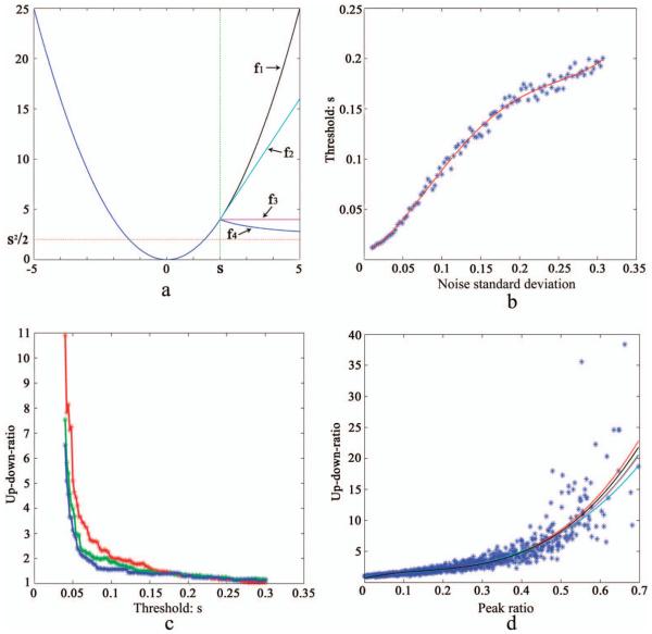
To deal with these limitations, we propose a new cost function, the asymmetric Indec function (see Fig. 1a):

$$\forall x\in R,\phi \left(x\right)=\{\begin{array}{cc}{x}^2,\hfill & \text{if}x<s\hfill \\ \frac{s^3}{2x}+\frac{s^2}{2},\hfill & \text{if}x\ge s\hfill \end{array}\phantom{\}}$$ (5)

Fig. 1.

Cost functions and choice of threshold. (a) Images of different cost functions. The combination of blue and black lines f₁ denotes the least squares penalty function, the combination of blue and cyan lines f₂ denotes the asymmetric Huber function, the combination of blue and magenta lines f₃ denotes the asymmetric truncated quadratic function, the combination of blue and blue lines f₄ denotes the asymmetric Indec function, and the red dotted line denotes the asymptote of the asymmetric Indec function. (b) Relationship between the noise standard deviation σ and the optimal threshold s. Blue star points denote the optimal threshold s that corresponds to a noise standard deviation σ; the red line is a fitted fourth-order polynomial based on these blue star points. (c) Relationship between threshold s and the up_down_ratio. Red, green, and blue star points denote the up_down_ratio that corresponds to a threshold s. (d) Relationship between the peak ratio and the up_down_ratio. The five polynomial curves denote five simulations, and each curve is fitted using 1000 star points.

We can see from the derivative of the asymmetric Indec function, φ′(x) = −s³/2x², that when the value of y_i − (Ta)_i > s, the change in cost increases faster as it moves upward, which effectively avoids the problem of the fitting curve moving away from the real baseline.

Minimization of the Cost Function

To minimize the criterion and obtain the polynomial coefficients, we can obtain the formula directly using the classical least squares approach:

$$a={\left(T^{T}T\right)}^{-1}{T}^{T}y$$ (6)

However, the minimization is not straightforward for all three functions.

In this paper, we use half-quadratic (HQ) minimization, which is an iterative technique simplifying the optimization of a non-quadratic criterion.^31,32 If f = φ(x) satisfies ∃α_max, ∀α [0, α_max], and g_α(x) = 0.5x² − αφ(x) is strictly convex, then we can use HQ minimization. To do this, we introduce an auxiliary vector d = [d₁, …, d_N] to solve for the polynomial coefficients a. For the asymmetric Indec function, we set α_max = 0.5 under the condition that s ≤ 2 (in polynomial fitting, we first standardize the data; then s will be less than 1). Then, we use the algorithm LEGEND to calculate a.³¹ To guarantee that g_α(x) is strictly convex and speed up the convergence, we set α = 0.99α_max, and initialize a as a = (T^TT)⁻¹T^Ty. Then, the two steps of iterations are as follows:

(1) When a is fixed, d is updated as: $d_i=-{\delta }_i+\alpha {\phi }^{\prime }\left({\delta }_i\right)\text{where}{\delta }_i=y_i-z_i=y_i-{\left(Ta\right)}_i$,

$$\phi \left(x\right)=\{\begin{array}{cc}{x}^2,\hfill & \text{if}x<s\hfill \\ \frac{s^3}{2x}+\frac{s^2}{2},\hfill & \text{if}x\ge s\hfill \end{array}\phantom{\}}$$ (7)

and the new d is represented as d = [d₁, …, d_N].

(2) Update a using the formula:

$$a={\left(T^{T}T\right)}^{-1}{T}^T(y+d)$$ (8)

The iteration stops when the change of a is smaller than a given threshold ε.

The Properties Between Threshold s and Other Parameters

When analyzing Raman data, we obtained three properties of threshold s and other parameters, which composed the theoretical foundation of our method.

Property 1: Threshold s Is Positively Correlated with the Noise Standard Deviation σ

In theory, the noise standard deviation σ determines the amplitude of the noise fluctuations, and the larger the amplitude, the larger the threshold s. This is also verified by the following experiment. We simulated 100 kinds of Raman spectra, each type with 10 different random baselines and the same noise standard deviation σ (1000 spectra in all). Then we obtained the optimal threshold s for each Raman spectrum. For each 10 Raman spectra with the same noise standard deviation σ, we calculated their average threshold s (ave-s) as Mazet et al.²⁸ did. The result (Fig. 1b) indicates that threshold s is positively correlated with the noise standard deviation σ.

Property 2: Threshold s Is Negatively Correlated with the Up_Down_Ratio

We define the up_down_ratio as the quotient of the number of points upward and downward from the baseline. We found that the larger the threshold s, the smaller the up_down_ratio. To verify this, we simulated three Raman spectra randomly and calculated their corresponding up_down_ratios. The threshold s values and their corresponding up_down_-ratios are graphed in Fig. 1c; this clearly indicates that the threshold s is negatively correlated with the up_down_ratio.

Property 3: A Cubic Polynomial Correlates the Up_Down_Ratio Shows with the Peak Ratio, and This Correlation is Hardly Influenced by the Noise Standard Deviation σ

The larger the peak ratio, the more points belong to the peaks of the Raman spectrum and the larger the up_down_ratio. In addition, for a given Raman spectrum with an explicit baseline and peaks, noise fluctuations with small σ hardly influence the up_down_ratio. We designed five experiments, each using a different noise standard deviations—0.02, 0.03, 0.04, 0.05, and 0.06—and each with 1000 simulated Raman spectra. We graphed the points of the peak ratio and up_down_ratio for all the Raman spectra and fitted the 1000 points in each experiment using a third-order polynomial. The points and curves are shown in Fig. 1d; we can see that these five curves almost coincide. This indicates that a cubic polynomial correlates the up_-down_ratio with the peak ratio and that this correlation is hardly influenced by noise standard deviation σ. The third-order polynomial we used for the algorithm design is y = 0.7679 + 11.2358x − 39.7064x² + 92.3583x³.

Choice of Polynomial Order p

Some algorithms can automatically estimate the polynomial order, for example, the Akaike information criterion (AIC).^28,33 However, we believe that the polynomial order should be a user-defined parameter, giving the researcher some degree of freedom. Generally speaking, the polynomial order determines the smoothness of the estimated baseline. If we need a smoother baseline, we choose a larger polynomial order p; otherwise we choose a smaller one. Indeed, some Raman spectra may have a part of the signal that can be alternatively considered a baseline or a peak, for example, the Raman spectral segment from 700 to 900 in Fig. 2. Adjusting the polynomial order p allows us to fit this part of the signal for each of these two cases.

Fig. 2.

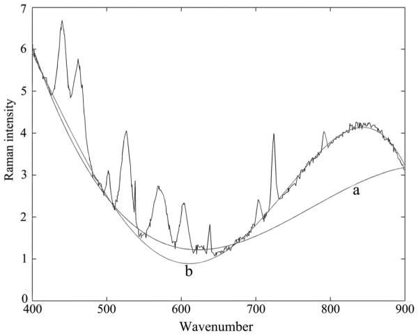
Estimation of the baseline with two different polynomial orders. Curve (a) is a third-order polynomial, and curve (b) is a fourth-order polynomial.

Designation of Algorithm Goldindec

We have discussed how to choose the polynomial order p for a given Raman spectrum. Another two input parameters are ε (default value 0.0001) and the peak ratio, which can be estimated from input data. Actually, based on our analysis, researchers can choose a peak ratio from 0.1 to 0.9 with step length 0.1 because Goldindec can fit a baseline with high accuracy within a 10% bias of the peak ratio. The details can be found in Results section. Given the two parameters ε and the peak ratio, Goldindec can correct the baseline using the following algorithm:³⁴

1. Calculate the up_down_ratio, denoted as r_ud, from the peak ratio based on the third-order polynomial between the peak ratio and the up_down_ratio, as described previously.

2. Initially, let a = 0 and b = , and calculate the tentative threshold s = a + 0.618(b − a); then compute the up_down_ratio using the current s and the algorithm LEGEND.

3. If |up_down_ratio − r_ud| ≤ ε, go to step 6; if up_down_ratio − r_ud > ε, go to step 4; if up_down_ratio − r_ud < −ε, go to step 5.

4. Let a = s, s = a + 0.618(b − a), and then compute the up_down_ratio using the current s and the algorithm LEGEND; then go to step 3.

5. Let b = s, s = a + 0.618(b − a), and then compute the up_down_ratio using the current s and the algorithm LEGEND; then go to step 3.

6. Stop the iteration, and calculate the final fitted baseline using the current s and the algorithm LEGEND.

RESULTS

Experiment Design and Data Acquisition

To compare the performance of Goldindec (e.g., accuracy and robustness) with other methods, we did experiments using both simulated and real Raman spectral data. The simulated Raman spectrum can be modeled as y = b + p + n, where b is the known polynomial function with an order less than six whose coefficients are generated from a zero-mean Gaussian with variance 1; p is the Raman spectroscopy peak function, which consists of a sparse spike train signal convolved with a Gaussian pulse; and n refers to the physical noise that is simulated by white Gaussian noise. We obtained real Raman spectral data for five minerals from the Handbook of Minerals Raman Spectra³⁵ database; the minerals contain different impurities and therefore different baselines. The minerals used are abelsonite (RRUFF³⁶ ID : R070007), adamite (R040130), fluorliddicoatite (R060635), marialite (R040043), and andersonite (R080133).

Algorithm Analysis

Accuracy Analysis of Threshold s

To evaluate the accuracy of threshold s given by Goldindec, we simulated 25 groups of Raman spectra data randomly and obtained the real threshold s (real-s); we also calculated the threshold s using Goldindec (opt-s); see Table I. The results indicate that the difference between real-s and opt-s is almost always less than 1%, with only two exceptions, 2.5 and 1.5%; this indicates that Goldindec computes threshold s with high accuracy.

TABLE I.

Comparison between real-s and opt-s.

Real-s	Opt-s	Error (%)
0.059	0.065	0.60
0.043	0.049	0.60
0.156	0.16	0.40
0.09	0.084	0.60
0.135	0.136	0.10
0.012	0.012	0
0.111	0.103	0.80
0.039	0.041	0.20
0.067	0.059	0.80
0.061	0.069	0.80
0.208	0.233	2.50
0.029	0.033	0.40
0.042	0.041	0.10
0.03	0.025	0.50
0.018	0.018	0
0.058	0.064	0.60
0.076	0.061	1.50
0.06	0.054	0.60
0.138	0.138	0
0.004	0.004	0
0.044	0.045	0.10
0.042	0.033	0.90
0.004	0.005	0.10
0.042	0.047	0.50
0.063	0.058	0.50

Robustness Analysis

The peak ratio estimated by researchers is usually not absolutely precise. To test the influence of the peak-ratio bias, we analyzed the robustness of Goldindec and defined the AC_rate, measuring the accuracy of the fitting result, as follows:

$$\begin{array}{cc}\hfill \text{Ac}\_\text{rate}& =1-\frac{\text{MD}}{\text{MD}\_\text{backgroud}},\hfill \\ \hfill & \text{where}\text{MD}=\sqrt{\frac{1}{N}\sum _{i=1}^N{(b-z)}^2},\hfill \\ \hfill & \text{MD}\_\text{background}=\sqrt{\frac{1}{N}\sum _{i=1}^N{b}^2}\hfill \end{array}$$ (9)

and where b refers to the real baseline, and z refers to the fitted polynomial baseline.

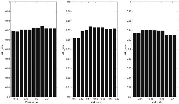
In this experiment, three groups of Raman spectra were generated randomly with known peak ratios, denoted pr. We constructed the bias interval [0.9pr, 1.1pr], divided into 10 equal intervals of 11 points. Then we fitted the baselines with the 11 points as the peak ratios and calculated their AC_rates. The results show that the accuracy of Goldindec remains stable within a 10% bias of the real peak ratio, indicating strong robustness (Fig. 3).

Fig. 3.

Robustness analyses of three groups of Raman spectra. The x-axis represents 11 values within a 10% bias of the real peak ratio, and the y-axis represents the fitting accuracy (AC_rate) of the corresponding peak ratio.

Because the robustness analysis of the peak ratio shows that Goldindec can fit the baseline with stable accuracy within a 10% bias of the real peak ratio, we can choose a value from 0.1 to 0.9 with step length 0.1 to estimate the peak ratio. These choices guarantee that the fitted baseline will have not only high accuracy but also very strong robustness. For example, if the real peak ratio is 24.7%, either 0.2 or 0.3 would be a reasonable choice.

Algorithm Efficiency Analysis

In this study, we adopted the 0.618 golden section iterative algorithm; thereby the length of search interval decreases exponentially in iterations, which ensures that the algorithm has a high computational efficiency. To test this, we generated 20 groups of Raman spectra randomly, and we fitted their baselines using Goldindec with ε = 0.0001. The numbers of iterative steps ranged from 12 to 17, indicating that Goldindec has high computational efficiency.

Result Analysis and Comparison Using Simulated Data

Comparison Between Two Cost Functions

Experiments showed that the asymmetric truncated quadratic function generates polynomial baselines more accurately than the asymmetric Huber function in Raman spectra. Thus, we need to compare only the asymmetric Indec function to the asymmetric truncated quadratic function.

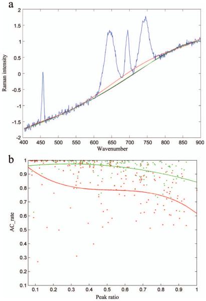
Compared to the asymmetric truncated quadratic function, the asymmetric Indec function has the property that the cost increases when the fitting curve moves upward and away from real baseline; thus, the fitted curve will be closer to the real baseline (Fig. 4a), which efficiently handles the limitations of the cost functions that are currently used. Furthermore, we adopted the AC_rate to measure the accuracy of the two cost functions and designed 100 experiments to compare them. For each experiment, we simulated a random Raman spectrum with a distinct peak ratio, and then we calculated the corresponding AC_rates of these two cost functions. Finally, we graphed the accuracy curves of two cost functions using the 100 AC_rates and peak ratios (Fig. 4b). The results show that the asymmetric Indec function performs better than the asymmetric truncated quadratic function, especially when the peak ratio is high.

Fig. 4.

(a) Comparison of the asymmetric truncated quadratic function and the asymmetric Indec function as cost functions. The blue curve represents the raw Raman spectrum, the black curve represents the real baseline, the green curve represents the fitted baseline with the asymmetric Indec function as the cost function, and the red curve represents the fitted baseline with the asymmetric truncated quadratic function as the cost function. Note that the black and green curves almost coincide, so it looks as if the black curve is missing. (b) The AC_rate curves of the asymmetric truncated quadratic function and the asymmetric Indec function as cost functions. The x-axis represents the peak ratios of 100 experiments, and the y-axis represents the corresponding AC_rate values. The red star points are the AC_rate values of the asymmetric truncated quadratic function as the cost function; the green star points are the AC_rate values of the asymmetric Indec function as the cost function; the red curve is a third-order polynomial fitted to the red star points; the green curve is a third-order polynomial fitted to the green star points.

Fig. 5.

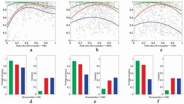
Comparison of Goldindec to two other methods using simulated data. Goldindec is in green, Paul’s method is in red, and Zhi-Min’s method is in blue. (a) Accuracy points and fitted curves with wavenumber 500. (b) Accuracy points and fitted curves with wavenumber 1000. (c) Accuracy points and fitted curves with wavenumber 1500. (d) Average accuracies and accuracy variations with wavenumber 500. (e) Average accuracies and accuracy variations with wavenumber 1000. (f) Average accuracies and accuracy variations with wavenumber 1500.

Accuracy Comparison with Other Methods

We then compared Goldindec³⁴ with another two baseline correction methods: Paul’s method³⁷ and Zhi-Min’s method.⁶ For the comparison, we generated three groups of Raman spectra, with wavenumber 500, 1000, or 1500, each containing 300 Raman spectra with different peak ratios. Then we calculated the AC_rates after applying the three methods to each group of Raman spectra. The accuracy curves are graphed for each method in Figs. 5a–5e. In addition, we calculated the average accuracy and accuracy variation for each group of Raman spectra (Fig. 5f). For Paul’s method, we chose the default value p = 0.01 and chose wavelength λ as the best one among 10⁴, 10⁵, …, 10⁹. For Zhi-min’s method, we chose λ as the best one among 10⁴, 10⁵, and 10⁶. The results showed that Goldindec performs better than the other two methods, having the highest average accuracy and lowest accuracy variation. In addition, the accuracy of Goldindec is hardly influenced by peak number. Goldindec achieved the highest accuracy using wavenumbers 500, 1000, and 1500. Although Paul’s method might not be influenced by wavenumber either, it has a high accuracy variation, indicating its instability. Zhi-Min’s method is not only influenced by wavenumber, but is also unstable.

Application Using Real Data and Comparison to Other Methods

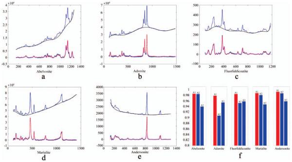
As mentioned, we obtained real Raman spectral data from the Handbook of Minerals Raman Spectra³⁵ database for five minerals with different impurities and thus different baselines. The baselines of these five minerals in this database were manually fitted by experts, and in this article, we take these experts’ results as the criteria for our comparison of Goldindec, Paul’s method, and Zhi-Min’s method. As we did in the last experiment, for Paul’s method we chose a default value p = 0.01 and chose λ as the best value among 10⁴, 10⁵, …, 10⁹. For Zhi-min’s method, we chose λ as the best value among 10⁴, 10⁵, and 10⁶. We again measured accuracy using AC_rate. The fitted results for Goldindec are displayed in Figs. 6a–6e. The results show that Goldindec accurately fitted the baseline for the Raman spectra of the five minerals. We can see that the fitted baselines almost coincide with the real ones determined by the database experts. The comparison in accuracy with the other two methods is shown in Fig. 6f; we can see that Goldindec has the highest accuracy among the three methods.

Fig. 6.

Comparison of Goldindec to two other methods using real data. (a) Fitting results of Goldindec for abelsonite. (b) Fitting results of Goldindec for adamite. (c) Fitting results of Goldindec for fluorliddicoatite. (d) Fitting results of Goldindec for marialite. (e) Fitting results of Goldindec for andersonite. The top blue curve in (a)–(e) represents the raw Raman spectroscopy, the black curve represents the fitted baseline, the blue curve below this represents the Raman spectrum corrected by Goldindec, and the red curve represents the Raman spectrum corrected by experts in the database. (f) Fitting accuracies of Goldindec (red bar, A1), Paul’s method (blue bar, A2), and Zhi-Min’s method (blue bar, A3) for the five mineral Raman spectra.

DISCUSSION

In this article, we have proposed a novel iterative algorithm, Goldindec, for polynomial fitting of the Raman spectrum baseline using a new cost function, the asymmetric Indec function. This cost function does not have the shortcomings of the asymmetric truncated quadratic function and has improved fitting accuracy, especially for Raman spectra with high peak numbers. In the analysis and experiments, we determined several properties of the parameters used in baseline fitting: (1) threshold s of the cost function is positively correlated with the noise standard deviation σ, (2) threshold s is negatively correlated with the up_down_ratio; and (3) a cubic polynomial correlates the up_down_ratio shows with the peak ratio, and this correlation is hardly influenced by peak variance σ. Based on these properties, we designed the 0.618 golden section iterative algorithm to automatically select a reasonable threshold s.

We compared Goldindec with another two methods using both simulated and real data. The results show that our algorithm has the highest accuracy when the peak ratio is not very high (less than 90%). Only when the peak ratio is more than 90%, which is rare in practice, does Zhi-Min’s method test a little better than Goldindec. Moreover, even though it may achieve a higher accuracy with higher peak ratios, the accuracy of Zhi-min’s method decreases when the peak ratio is low and is unstable under the influence of noise. In fact, no polynomial fitting method works very well when the peak ratio is very high; therefore, we will try combining other methods to solve the problem of high peak ratios in future studies.

References

- 1.Lau SK, Winlove P, Moger J, Champion OL, Titball RW, Yang ZH, Yang ZR. A Bayesian Whittaker–Henderson Smoother for General-Purpose and Sample-Based Spectral Baseline Estimation and Peak Extraction. J. Raman Spectrosc. 2012;43(9):1299–1305. [Google Scholar]
- 2.Puppels COGJ, Greve J, Robert-Nicoud M, Arndt-Jovin DJ, Jovin TM. Raman Microspectroscopic Study of Low-pH-Induced Changes in DNA Structure of Polytene Chromosomes. Biochemistry. 1994;33(11):3386–3395. doi: 10.1021/bi00177a032. [DOI] [PubMed] [Google Scholar]
- 3.Duguid J, Bloomfield VA, Benevides J, Thomas GJ., Jr Raman Spectroscopy of DNA-Metal Complexes. I. Interactions and Conformational Effects of the Divalent Cations: Mg, Ca, Sr, Ba, Mn, Co, Ni, Cu, Pd, and Cd. Biophys. J. 1993;65(5):1916–1928. doi: 10.1016/S0006-3495(93)81263-3. [DOI] [PMC free article] [PubMed] [Google Scholar]
- 4.Tuma R. Raman Spectroscopy of Proteins: From Peptides to Large Assemblies. J. Raman Spectrosc. 2005;36(4):307–319. [Google Scholar]
- 5.Baek SJ, Park A, Shen AG, Hu JM. A Background Elimination Method Based on Linear Programming for Raman Spectra. J. Raman Spectrosc. 2011;42(11):1987–1993. [Google Scholar]
- 6.Zhang ZM, Chen S, Liang YZ. Baseline Correction Using Adaptive Iteratively Reweighted Penalized Least Squares. Analyst. 2010;135(5):1138–1146. doi: 10.1039/b922045c. [DOI] [PubMed] [Google Scholar]
- 7.Mittermayr CR, Tan HW, Brown SD. Robust Calibration with Respect to Background Variation. Appl. Spectrosc. 2001;55(7):827–833. [Google Scholar]
- 8.Tan HW, Brown SD. Wavelet Analysis Applied to Removing Non-Constant, Varying Spectroscopic Background in Multivariate Calibration. J. Chemom. 2002;16(5):228–240. [Google Scholar]
- 9.Gemperline PJ, Cho JH, Archer B. Multivariate Background Correction for Hyphenated Chromatography Detectors. J. Chemom. 1999;13(2):153–164. [Google Scholar]
- 10.Likar A, Vidmar T. A Peak-Search Method Based on Spectrum Convolution. J. Phys. D-Appl. Phys. 2003;36(15):1903–1909. [Google Scholar]
- 11.Shusterman V, Shah SI, Beigel A, Anderson KP. Enhancing the Precision of ECG Baseline Correction: Selective Filtering and Removal of Residual Error. Comput. Biomed. Res. 2000;33(2):144–160. doi: 10.1006/cbmr.2000.1539. [DOI] [PubMed] [Google Scholar]
- 12.Xu YM, Lin QZ, Wang L, Wang QJ. The Prediction of Nitrogen Concentration in Soil by VNIR Reflectance Spectrum; Proceedings of the 2005 IEEE International Geoscience and Remote Sensing Symposium 2005 (IGARSS ’05); New York. 2005. pp. 4451–4454. IEEE. doi:10.1109/IGARSS.2005.1525908. [Google Scholar]
- 13.Schulze G, Jirasek A, Yu MML, Lim A, Turner RFB, Blades MW. Investigation of Selected Baseline Removal Techniques as Candidates for Automated Implementation. Appl. Spectrosc. 2005;59(5):545–574. doi: 10.1366/0003702053945985. [DOI] [PubMed] [Google Scholar]
- 14.Asfour H, Swift LM, Sarvazyan N, Doroslovacki M, Kay MW. Signal Decomposition of Transmembrane Voltage-Sensitive Dye Fluorescence Using a Multiresolution Wavelet Analysis. IEEE Trans. Biomed. Eng. 2011;58(7):2083–2093. doi: 10.1109/TBME.2011.2143713. [DOI] [PMC free article] [PubMed] [Google Scholar]
- 15.Du JQ, Wu XM, Zhang HQ, Wang SA, Tan WH, Guo XO. Mass Spectrometry-Based Proteomic Analysis of Kashin-Beck Disease. Mol. Med. Rep. 2010;3(5):821–824. doi: 10.3892/mmr.2010.327. [DOI] [PubMed] [Google Scholar]
- 16.Chen D, Chen ZW, Grant E. Adaptive Wavelet Transform Suppresses Background and Noise for Quantitative Analysis by Raman Spectrometry. Anal. Bioanal. Chem. 2011;400(2):625–634. doi: 10.1007/s00216-011-4761-5. [DOI] [PubMed] [Google Scholar]
- 17.Zhang ZM, Chen S, Liang YZ. Peak Alignment Using Wavelet Pattern Matching and Differential Evolution. Talanta. 2011;83(4):1108–1117. doi: 10.1016/j.talanta.2010.08.008. [DOI] [PubMed] [Google Scholar]
- 18.Indic P, Narayanan J. Wavelet Based Algorithm for the Estimation of Frequency Flow from Electroencephalogram Data During Epileptic Seizure. Clin. Neurophysiol. 2011;122(4):680–686. doi: 10.1016/j.clinph.2010.10.030. [DOI] [PubMed] [Google Scholar]
- 19.Nguyen N, Huang H, Oraintara S, Vo A. Mass Spectrometry Data Processing Using Zero-Crossing Lines in Multi-Scale of Gaussian Derivative Wavelet. Bioinformatics. 2010;26(18):i659–i665. doi: 10.1093/bioinformatics/btq397. [DOI] [PMC free article] [PubMed] [Google Scholar]
- 20.Du P, Kibbe WA, Lin SM. Improved Peak Detection in Mass Spectrum by Incorporating Continuous Wavelet Transform-Based Pattern Matching. Bioinformatics. 2006;22(17):2059–2065. doi: 10.1093/bioinformatics/btl355. [DOI] [PubMed] [Google Scholar]
- 21.Ressom HW, Varghese RS, Drake SK, Hortin GL, Abdel-Hamid M, Loffredo CA, Goldman R. Peak Selection from MALDI-TOF Mass Spectra Using Ant Colony Optimization. Bioinformatics. 2007;23(5):619–626. doi: 10.1093/bioinformatics/btl678. [DOI] [PubMed] [Google Scholar]
- 22.Li JS, Yu BL, Zhao WX, Chen WD. A Review of Signal Enhancement and Noise Reduction Techniques for Tunable Diode Laser Absorption Spectroscopy. Appl. Spectrosc. Rev. 2014;49(8):666–691. [Google Scholar]
- 23.Li J, Yu B, Fisher H. Wavelet Transform Based on the Optimal Wavelet Pairs for Tunable Diode Laser Absorption Spectroscopy Signal Processing. Appl. Spectrosc. 2014;69(4):496–506. doi: 10.1366/14-07629. [DOI] [PubMed] [Google Scholar]
- 24.Zhao J, Lui H, McLean DI, Zeng H. Automated Autofluorescence Background Subtraction Algorithm for Biomedical Raman Spectroscopy. Appl. Spectrosc. 2007;61(11):1225–1232. doi: 10.1366/000370207782597003. [DOI] [PubMed] [Google Scholar]
- 25.Mosier-Boss PA, Lieberman SH, Newbery R. Fluorescence Rejection in Raman Spectroscopy by Shifted-Spectra, Edge Detection, and FFT Filtering Techniques. Appl. Spectrosc. 1995;49(5):630–638. [Google Scholar]
- 26.Mahadevan-Jansen A, Richards-Kortum RR. Raman Spectroscopy for the Detection of Cancers and Precancers. J. Biomed. Opt. 1996;1(1):31–70. doi: 10.1117/12.227815. [DOI] [PubMed] [Google Scholar]
- 27.Lieber CA, Mahadevan-Jansen A. Automated Method for Subtraction of Fluorescence from Biological Raman Spectra. Appl. Spectrosc. 2003;57(11):1363–1367. doi: 10.1366/000370203322554518. [DOI] [PubMed] [Google Scholar]
- 28.Mazet V, Carteret C, Brie D, Idier J, Humbert B. Background Removal from Spectra by Designing and Minimising a Non-Quadratic Cost Function. Chemom. Intell. Lab. Syst. 2005;76(2):121–133. [Google Scholar]
- 29.Vickers TJ, Wambles RE, Mann CK. Curve Fitting and Linearity: Data Processing in Raman Spectroscopy. Appl. Spectrosc. 2001;55(4):389–393. [Google Scholar]
- 30.Goehner RP. Background Subtract Subroutine for Spectral Data. Anal. Chem. 1978;50(8):1223–1225. [Google Scholar]
- 31.Idier J. Convex Half-Quadratic Criteria and Interacting Auxiliary Variables for Image Restoration. IEEE Trans. Image Process. 2001;10(7):1001–1009. doi: 10.1109/83.931094. [DOI] [PubMed] [Google Scholar]
- 32.Geman D, Yang C. Nonlinear Image Recovery with Half-Quadratic Regularization. IEEE Trans. Image Process. 1995;4(7):932–946. doi: 10.1109/83.392335. [DOI] [PubMed] [Google Scholar]
- 33.Akaike H. A New Look at the Statistical Model Identification. IEEE Trans. Autom. Control. 1974;19(6):716–723. [Google Scholar]
- 34.Goldindec (Baseline_Correction) Transcriptome Assembly. SourceForge. 2015 http: //sourceforge.net/projects/transcriptomeassembly/files/Baseline_Correction/Goldindec.rar/download.
- 35.Laboratoire de gé ologie de Lyon . Handbook of Minerals Raman Spectra [database] ENS-Lyon France: 2000-2015. http://www.ens-lyon.fr/LST/Raman/ [Google Scholar]
- 36.Downs RT. The RRUFF Project: An Integrated Study of the Chemistry, Crystallography, Raman and Infrared Spectroscopy of Minerals; Program and Abstracts of the 19th General Meeting of the International Mineralogical Association in Kobe, Japan, July 23-28, 2006; IMA. 2006. p. 117. O03-13. [Google Scholar]
- 37.Eilers PHC, Boelens HFM. Leiden University Medical Centre Report. Leiden University Medical Centre; Leiden: 2005. Baseline Correction with Asymmetric Least Squares Smoothing. [Google Scholar]