

Abstract
In this study, we used invasive tracing to evaluate white matter tractography methods based on ex vivo diffusion‐weighted magnetic resonance imaging (dwMRI) data. A representative selection of tractography methods were compared to manganese tracing on a voxel‐wise basis, and a more qualitative assessment examined whether, and to what extent, certain fiber tracts and gray matter targets were reached. While the voxel‐wise agreement was very limited, qualitative assessment revealed that tractography is capable of finding the major fiber tracts, although there were some differences between the methods. However, false positive connections were very common and, in particular, we discovered that it is not possible to achieve high sensitivity (i.e., few false negatives) and high specificity (i.e., few false positives) at the same time. Closer inspection of the results led to the conclusion that these problems mainly originate from regions with complex fiber arrangements or high curvature and are not easily resolved by sophisticated local models alone. Instead, the crucial challenge in making tractography a truly useful and reliable tool in brain research and neurology lies in the acquisition of better data. In particular, the increase of spatial resolution, under preservation of the signal‐to‐noise‐ratio, is key. Hum Brain Mapp 36:4116–4134, 2015. © 2015 The Authors Human Brain Mapping Published by Wiley Periodicals, Inc.
Keywords: MRI, brain connections, DTI, crossing fibers, white matter, tracking
INTRODUCTION
Tractography is a class of techniques that aim to extract information about white matter fiber systems from diffusion‐weighted magnetic resonance imaging (dwMRI) data [e.g., Kaden et al., 2007; Mori and van Zijl, 2002; Mori et al., 1999; Tournier et al., 2011]. While the resulting fiber pathways certainly contain valuable information about the underlying architecture, they are subject to a number of serious pitfalls and limitations [Jones, 2010; Jones and Cercignani, 2010; Jones et al., 2012]. In order to assess the confidence we may place in results from different tractography methods and to gain deeper insight into the nature of the various problems, validation against a “ground truth” would be invaluable. However, such a ground truth regarding the fiber connectivity within the entire brain is very difficult to obtain. Although classical in vivo tracing techniques in animals yield very accurate quantitative estimates of the connectivity, they can typically only be applied to just one injection site per animal, and require painstaking procedures [e.g., Dauguet et al., 2007; Schmahmann et al., 2007]. For example, in a recent study Jbabdi and colleagues [2013] successfully used tracers for long‐range connections of the ventral prefrontal cortex in macaque monkeys and compared this to ex vivo tractography.
On the other hand, in vivo manganese tracers can be visualized by magnetic resonance imaging (MRI) and thereby used to characterize the connectivity of an injection site with the entire brain, which is very comparable to the connectivity profile of a seed region obtained by tractography [Dyrby et al., 2007; Gutman et al., 2013; Lin et al., 2001]. Therefore, manganese is an excellent means of validating diffusion tractography. However, because it is inevitable that the substance is not completely taken up by the cells and then transported down the axons, but also diffuses in intra‐axonal space, some extra calibration is needed, which is provided by a histochemical tracer. Dyrby and colleagues [2007] used this technique to assess the performance of a multitensor probabilistic tractography method and showed by direct comparison (the same brain that received a tracer was also imaged) a generally high agreement between tracer and tractography results, which was reproducible across brains. However, they also demonstrated that well‐known sources of error, such as regions with crossing fibers, impact upon the performance of the tractography. Over time, a whole range of tractography methods have emerged that primarily aim to ameliorate these problems. Hence, it is important to assess, using the same validation method, to what extent and under which circumstances these different methods succeed in doing so.
Therefore, we applied a representative selection of tractography techniques to ex vivo diffusion data in pig brains, involving both probabilistic [Behrens et al., 2007; Descoteaux et al., 2009; Kaden et al., 2007] and deterministic [Conturo et al., 1999; Lazar et al., 2003; Mori et al., 1999] tracking algorithms, as well as local models (fitted to the data in a voxel‐wise way) based on single tensors [Basser et al., 1994], multiple compartments [Behrens et al., 2003; Liu et al., 2004; Tuch et al., 2002], and diffusion fiber orientation density functions (ODF) [Aganj et al., 2010; Alexander, 2005b; Dell'Acqua et al., 2010; Descoteaux et al., 2007; Patel et al., 2010; Tournier et al., 2007; Tournier et al., 2004; Tuch, 2004]. Moreover, in order to cope with the well‐known path length dependence of probabilistic tractography scores, we used a novel method called iterative confidence enhancement for tractography (ICE‐T) [Liptrot et al., 2014]. This method is applied as a wrapper to existing probabilistic tractography methods. In contrast to our previous work [Dyrby et al., 2007], where waypoint masks were utilized to reduce the incidence of false positives, we did not use any additional constraint other than the seed region.
First, we will report a systematic quantitative assessment of the specificity and sensitivity of the different methods with respect to manganese tracing and their dependence upon the threshold settings. Second, we will discuss, in detail, the qualitative performance of the different methods in terms of reaching the relevant tract systems, their robustness toward threshold settings, and the occurrence of spurious connections (false positives). The software packages we used to run the various tractography algorithms offer a number of changeable parameters. We used the default parameter settings, as far as possible. In addition, although a complete parameter study would have been beyond the scope of this article, we investigated the impact of varying the most important parameters of each method.
We demonstrate that typical difficulties for tractography, such as crossing fibers, high curvature (relative to the image resolution), and long path lengths, are problematic for all methods in a similar way. However, models that are able to account for complex fiber layouts within a voxel do perform better in some cases. In fact, with current methods and data, valid results with few false positives can be obtained, but at the expense of not finding all true tracts. We conclude that further sophistication of local models and tractography algorithms might only unfold its full potential for the reconstruction of more details of the fiber architecture, if they are combined with better data, that is, higher spatial and angular resolution, higher signal‐to‐noise ratio (SNR), more and higher b‐values.
MATERIALS AND METHODS
Manganese Tracing
Manganese maps of three young, normal Göttingen mini pig brains (P1, P2, P3) used in a previous study [Dyrby et al., 2007] were re‐used here for tractography validation. Each of the three brains had received a single injection, comprising two in vivo tracers, in either the left motor cortex (MC), the right somatosensory area (SC), or the right prefrontal cortex (PFC). Two types of tracers had been employed: manganese, a paramagnetic tracer visualized in vivo on T1‐weighted MRI, and biotinylated dextran amine (BDA), a histochemical tracer. Manganese t‐score maps were computed by comparing 16 repetitions of T1w images two days before manganese injection with 16 repetitions on day 2 after injection [Dyrby et al., 2007]. Because not the entire manganese is taken up by the neurons and then transported along the axons, there is also significant manganese concentration diffusing in the extracellular space, especially around the injection site. In order to reduce the bias caused by that background signal, we need to define a suitable threshold for the t‐score map, which lies above the normal significance threshold (e.g., P < 0.05). While for the quantitative comparison (see below) we systematically varied that threshold, for the qualitative comparison (see below) we optimized the threshold for defining the seed region‐of‐interest (ROI) such that, within the injection area of the BDA, the tracer signal and the manganese positive volume coincided as much as possible.
Visualization procedures for the manganese in vivo tracer (manganese t‐maps), and the method by which t‐maps obtained from P2 and P3 were warped onto the image space of P1 that is used for tractography in this study are described elsewhere [Dyrby et al., 2007] and are made available at http://dig.drcmr.dk/downloads upon publication of this article. The brains had all been perfusion fixated, following the procedure described in [Dyrby et al., 2011]. All procedures followed the Guidelines for the Care and Use of Experimental Animals and were approved by the Danish Animal Experiments Inspectorate.
Magnetic Resonance Imaging
The ex vivo diffusion‐weighted MRI dataset of P1 used in this study was originally described by Dyrby et al. [2007]. It was acquired on a preclinical 4.7T Varian MR scanner using a pulse gradient spin echo (PGSE) sequence (TR = 6,500 ms, TE = 67.1 ms; voxel resolution 0.51 × 0.51 × 0.5 mm2) with a b‐value of 4009 s/mm2 (gradient duration, δ = 27 ms; time between gradient‐pulse onsets, Δ = 33.5 ms; gradient strength 56 mT/m), as specified in Dyrby et al. [2011].
Note that the relatively high b‐value was chosen, because the diffusivity in postmortem tissue is approximately one‐third of the in vivo value [D'Arceuil et al., 2007; Dyrby et al., 2011; Sun et al., 2005]. This should make the angular attenuation profile similar to the one obtained in living tissue with a b‐value of about 1,300 s/mm2, which is close to commonly used values in clinical scanners. We can afford to use such a high b‐value, because the main disadvantage of this choice, that is, lowered SNR can be easily compensated by prolonged scanning and the use of smaller volume radio frequency (RF) coils designed for fixed brain tissue.
The diffusion‐weighted MRI dataset included 3 scans with b = 0 s/mm2, and 61 diffusion encoding directions with a NEX of 2. The brain tissue had been stabilized to room temperature before MR scanning, and a dummy run lasting 15 h had been implemented to avoid the introduction of short‐term instabilities in the diffusion MRI dataset [Dyrby et al., 2011].
Seed Regions
Three seed ROIs were drawn on the dataset from P1: in the right PFC, in the right SC and in the left MC. The seed ROIs were the same as those used by Dyrby et al., [2007] (http://dig.drcmr.dk/downloads) and were manually drawn with the guidance of the three injection sites identified from the (warped) t‐maps of the manganese tracer. Note that the seed region is used differently by the different tractography algorithms: probabilistic tractography is seeded only in the seed region (local seeding), while deterministic tractography is seeded in the entire brain with subsequent selection of the fibers that pass through the seed region (global seeding).
Tractography Methods
We selected a set of tractography methods to include some of the most commonly used techniques and sample the most important algorithmic choices, such as probabilistic versus deterministic tracking and single tensor versus multi‐compartment and constrained spherical deconvolution (CSD) local models. Moreover, the recently proposed ICE‐T [Liptrot et al., 2014] was considered. Each of the methods has been published and most of them are included in publically available software packages. The methods involve certain parameter choices, such as fractional anisotropy (FA) thresholds. The parameters chosen for each algorithm were mostly following the default values given by the respective software developers. This ensured that the algorithms were used in the same manner as that chosen by most other users. In some cases, parameters were changed to match the special properties of our pig brains as opposed to the normally used human brains (in particular the FA threshold). In addition, we also explored the influence of the variation of some of the most important parameters, although a full‐fledged parameter study of all algorithms was considered beyond the scope of this work.
Deterministic diffusion tensor
We used the diffusion tensor (DT) model [Basser et al., 1994], which assumes a Gaussian distribution to approximate the diffusion propagator. The principal eigenvector of the tensor is usually interpreted as the main fiber direction and used for streamline tracking [Mori et al., 1999]. The tracts are computed by integrating the vector field of these principal eigenvectors. A drawback of this approach is that the tensor information beyond the first eigenvector is disregarded. In other words, an almost round tensor with very weak directionality has the same impact as a very pointed one. An alternative approach is the tensor deflection method [Lazar et al., 2003] implemented in MedINRIA (Version 1.6, http://www-sop.inria.fr/asclepios/software/MedINRIA), which will be used in this study.
One streamline was started in the center of every white matter voxel with a FA value > 0.13, and subsequently terminated upon reaching the boundaries of the white‐matter mask defined by this FA threshold. Note that this critical FA value was chosen to separate gray and white matter in our postmortem pig data and differs from those usually optimal for in vivo human data (FA > 0.2). All lines shorter than 10 mm were excluded and the smoothness parameter in MedINRIA was set to 10. Finally, only those streamlines crossing the seed area were retained from this whole brain tracking result. A connectivity map was created by counting the number of streamlines crossing each voxel (streamline count map).
Deterministic constrained spherical deconvolution
To model the distribution of crossing fibers in each voxel, we computed the fiber orientation density function (fODF) by CSD [Tournier et al., 2007], based on spherical harmonics of order 6, as implemented in MRTrix (http://www.brain.org.au/software/mrtrix). Note that CSD with higher order harmonics (order 8) has already been successfully used in in vivo human data with b = 3,000 s/mm2 [Tournier et al., 2009]. However, with our postmortem data (which are comparable to human data with b = 1,300 s/mm2, see above) that choice turned out instable. We have shown previously that in human data with b = 1,000 s/mm2 and 60 directions, CSD with sixth order harmonics was stable and capable of resolving fiber crossings of up to three bundles [Riffert et al., 2014].
The FA threshold for the computation of the deconvolution kernel was 0.7. Whole brain deterministic streamline tracking was initialized in all brain voxels. The brain mask, including gray and white matter as possible seed points, was generated using a low (FA > 0.13) threshold. The tracking algorithm followed all local maximum directions with a fODF value > 0.1. The tracking procedure repeatedly selected a random initialization point within the brain mask and started a new streamline until a total of 100,000 streamlines with a minimum length of 10 mm were computed. Only those streamlines crossing the seed area were selected and used for the computation of the streamline count map.
Probabilistic DT
We used the particle jump algorithm proposed by Koch et al. [2002], with the 3D implementation [Anwander et al., 2007]. This method samples the transition probability between neighboring voxels from a sharpened version of the neighboring tensors and uses the sampled values in a random‐walk algorithm. Note that the term “probabilistic,” though commonly used, is not entirely correct here, as the tensor describes a probability distribution of the water diffusion and not of the fiber orientation. Although there is a relation between the two, more formally correct approaches have been proposed [Jones and Pierpaoli, 2005]. Here, however, we stick to the approach and terminology that is commonly used.
The algorithm was initialized by 100,000 particles in the seed region and the tracking space was limited by a mask of FA > 0.05. Finally, the dynamic range of the streamline count map was reduced by logarithmic transformation.
Probabilistic ball and stick
The multiple ball‐and‐stick (B&S) model decomposes the diffusion‐weighted MRI signals into an isotropic (ball) and several anisotropic (sticks) compartments. The latter represent estimates for the principal fiber directions. In the work of Behrens et al. [2007], a fixed maximal number of sticks were used for each voxel. Herein, however, the number of directions supported by the data in each voxel was computed by automatic relevance determination. For each of these directions, an indicator of their creditability according to the diffusion‐weighted MRI data was determined. The direction of a stick was only used when its indicator was above a threshold computed by the algorithm, which means it was supported by the data. Here, we used the probtrackx procedure implemented in FSL (http://fsl.fmrib.ox.ac.uk/fsl/fsl-4.1.9/fdt/fdt_probtrackx.html; version 4.1.9). The probabilistic tracking was initialized in the seed region using default parameters of 5,000 samples per voxel and up to two sticks per voxel. As stopping criteria, a curvature threshold of 0.2 and a maximum of 2,000 steps were used.
Probabilistic multi‐tensor
Probabilistic tractography based on the multiple DT (MDT) model [Alexander, 2005a] implemented in the software Camino [Cook et al., 2006] was used following the same setup as was used by Dyrby et al. [2007], except that here we did not use any additional constraints other than the seed ROIs. In contrast, Dyrby and colleagues [2007] used constrained tractography for extracting specific pathways via waypoint ROIs. The MDT model was fitted to the diffusion‐weighted MRI data set. The number of tensors to be initially fitted in each voxel was determined from the classification algorithm by Alexander et al. [2002]. The stepwise projection of streamlines used a modified non‐interpolated fiber assignment by continuous tracking (FACT) method [Mori et al., 1999) with 64,000 streamlines starting from the seed area. The stopping criteria comprised a maximal curvature of 80° within a single voxel and the propagation into non‐brain voxels.
Probabilistic multi‐tensor with ICE‐T
We applied the ICE‐T framework to the probabilistic multi‐tensor method described above to address the path‐length dependency issue inherent in probabilistic methods [Liptrot et al., 2014]. The ICE‐T framework iteratively grows the seed region by binarizing the confidence map generated by probabilistic tracking at the ICE‐Tthreshold and uses that as an extended seed region for the next iteration. The iterative process stops when the seed region has stopped growing. Here, the final seed region after growing was then used as the seed region for MDT probabilistic tractography. ICE‐T has two parameters: ICE‐Tthreshold controls which supra‐threshold voxels are aggregated into the current seed region for the next iteration and was set to 0.01, ICE‐Tstreams determines the number of streamlines per voxel per iteration and was set to 20. These values have been shown to be suitable for efficiently growing a seed region along the tract system [Liptrot et al., 2014].
Global Voxel‐Wise Assessment
To evaluate the global agreement between manganese tracing and tractography, we computed a number of measures which were based on the assumption that manganese represents the ground truth. As a basis, we computed the numbers of “true positives” (TP; voxels that were positive in both manganese tracing and tractography), “false positives” (FP; voxels that were positive in tractography but negative in manganese tracing), “true negatives” (TN; voxels that were negative in both methods), and “false negatives” (FN; voxels that were positive in manganese tracing, but negative in tractography). From that, we derived the “sensitivity” by computing the fraction of manganese positive voxels (according to our assumption, the “truly” connected voxels) that were also detected by tractography: SENS = TP/(TP + FN), and the “specificity” by computing the fraction of tractography positive voxels that were also found by tracing: SPEC = TP/(TP + FP). These measures depended upon thresholding of the images to decide whether a certain voxel was considered positive or negative. Both thresholds varied between 0 and 100% of the image maximum (the maximum connectivity or streamline count value, which is usually reached in the seed region) and the measures were plotted as function of them.
Voxels within a distance of 10 mm of the injection site were ignored because extracellular diffusion of the manganese renders tracing unreliable in that area.
Qualitative Assessment
In order to obtain qualitative insight into the ability of tractography to reconstruct certain pathways, we first determined, for each injection site, a suitable manganese threshold for which all the tracts that were also identified by the histochemical BDA tracing would be found [Dyrby et al., 2007], with as little unspecific spreading around the injection site as possible (see Appendix for the values). Then, we varied the thresholds for the tractography methods in order to assess the relationship between sensitivity (finding all tracts) and specificity (not finding false tracts) and, where possible, to identify an optimal compromise between the two.
RESULTS
Global Voxel‐Wise Assessment
Here, we studied the threshold‐dependent voxel‐wise overlap between manganese tracing and diffusion tractography in order to assess the sensitivity and specificity of the different tractography algorithms. For example, for the injection site in the prefrontal cortex (PFC), high thresholds for the manganese tracing images (>50% of the range) limited the connected voxels to the vicinity of the injection site. Lowering the threshold to about 40% resulted in the appearance of initial sections of the pathways. At threshold levels of about 20% all tracts were revealed down to their respective targets, while further lowering led to implausible connectivity estimates covering large parts of the brain. See also Figure 1. Similar observations were made for the other two injection sites (results not shown).
Figure 1.
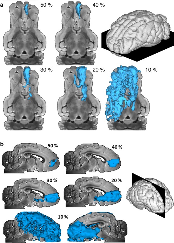
Top axial (a) and right sagittal (b) views of a three‐dimensional isosurface representation of manganese tracing from the PFC injections site, at different thresholds (as percentage of the maximal range). The 10% image is shown from, both, the left and right sides, because with this low threshold the connected volume extends to both hemispheres. [Color figure can be viewed in the online issue, which is available at http://wileyonlinelibrary.com.]
Accordingly, for very low manganese thresholds (ca. 10% and less), specificity went mostly to unity and sensitivity dropped to zero for all methods, irrespective of the tractography threshold (Fig. 2). On the other hand, for manganese threshold above about 50%, the scores referred only to restricted areas near the injection site. The interesting range of manganese thresholds is between 20 and 40–50%. In that range, we generally observed that sensitivity was very low and fairly independent of tractography thresholds (except for extremely low tractography thresholds, where almost the entire brain appeared connected). One exception was the probabilistic tensor tractography, yet even here no threshold combination existed that provided acceptable specificity and sensitivity at the same time. This meant that most of the voxels that were connected in the manganese image, at any threshold that insured that the tracing reached the putative target sites, were not found by any of the tested tractography methods or, in the case of the probabilistic tensor method, were associated with a large number of false positives.
Figure 2.
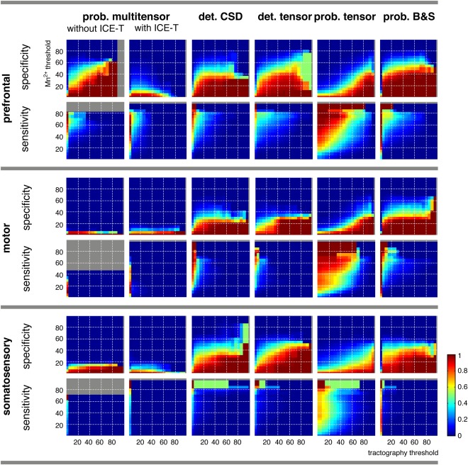
Plots of voxel‐wise sensitivity and specificity of different tractography methods with respect to manganese tracing, as a function of manganese and tractography thresholds. See text for detailed explanation. The gray areas indicate threshold combinations where a computation was not possible, because there were no manganese positive (for sensitivity) or no tractography position (for specificity) voxels, respectively. Note that the radius = 1 cm environment of the injection site was excluded from analysis. [Color figure can be viewed in the online issue, which is available at http://wileyonlinelibrary.com.]
To what extent these problems may be more fundamental in nature, such as whether or not manganese‐positive fiber tracts are actually attainable with tractography, or whether they may just be due to the fact that tractography stays in a narrower channel whilst following the main fiber direction, is left as a question for the qualitative assessment (next section). In contrast to sensitivity, specificity is quite high for all tractography methods, meaning that most of the voxels reached by tracking are “true,” as defined by manganese. However, there are varying degrees of tractography threshold dependence. For example, the B&S method can reach 100% specificity for most tractography thresholds, provided that the manganese threshold is sufficiently low. However, the specificity is much lower for very low tractography thresholds, exactly where the sensitivity reaches acceptable levels (see also the choice of the thresholds for the quantitative analysis, Tab. 1). On the other hand, probabilistic tensor tractography needs rather high tractography thresholds for most manganese thresholds. Interestingly, the multiple tensor tracking with ICE‐T showed, for two of the injection sites, an increase in specificity toward lower tractography thresholds, which was in contrast to all other methods. This might indicate some systematic deviation between tracing and tracking. In contrast to all the other tracking methods, ICE‐T demonstrates minimal dependency upon the threshold.
Table 1.
Overview on the qualitative assessment of the tractography performance
| Injection | Projection | DT det | CSD det | DT prob | B&S | MDT | MDT + ICE‐T | |
|---|---|---|---|---|---|---|---|---|
| right PFC | true | SN | (√)a | √ | (√)a | (√)b | √ | √ |
| MD | — | — | — | — | — | — | ||
| cPFC | (√)a | √ | √ | √ | √ | √ | ||
| false | SL | × | × | × | × | — | — | |
| CE | × | × | × | — | — | — | ||
| Cing | — | × | × | × | — | — | ||
| FSC | × | — | — | — | — | — | ||
| ventral PFC | — | — | — | — | × | × | ||
| near injection | — | — | — | × | — | — | ||
| left MC | true | VA/VL | (√)a | √ | √ | √ | √ | √ |
| Cd | — | — | — | — | — | — | ||
| cMC | (√)a | (√)a | (√)a | (√)a | (√)a | √ | ||
| false | CI | × | — | × | — | — | — | |
| cCI/CE | — | × | × | × | — | — | ||
| Fx | × | — | — | — | — | — | ||
| PFC | × | — | — | — | — | — | ||
| near injection | — | — | × | × | — | — | ||
| other contra | — | — | — | — | — | × | ||
| right SC | true | SN | (√)c | (√)c | — | — | (√)c | (√)c |
| VP/VPL | — | (√)c | — | (√)3 | — | — | ||
| cSC | (√)c | (√)c | (√)a | (√)c | (√)c | (√)c | ||
| false | FSC | × | — | — | × | — | — | |
| ventral PFC | × | — | — | — | — | — | ||
| CE | × | — | × | — | ||||
| Cing | — | — | — | × | — | — | ||
| Fx | — | — | — | × | — | — | ||
| BS | — | — | × | — | — | — | ||
| cCI | — | — | — | × | — | — | ||
| near injection | × | × | × | × | × | ×d | ||
True positive connections labeled with √ if present. If the path was not followed to the end (“destination not reached”) or took a similar, but deviating trajectory (√) war used. False positive connections are labeled with × if present. See text and Figures 3, 4, 5 for more details.
Anatomical labels: SN; substantia nigra; MD; medio‐dorsal nucleus of thalamus; (c)PFC; (contralateral) prefrontal cortex; SL; nucleus septalis lateralis; CE; external capsule; (c)CI; (contralateral) internal capsule; Cing; cingulum; FSC; subcallosal fasciculus; VA/VL; ventro‐anterior/ventro‐lateral thalamus; Cd; caudate nucleus; (c)MC; (contralateral) motor cortex; Fx; fornix; VP/VPL; ventral posterior/ventral posterior lateral thalamus; (c)SC; (contralateral) somatosensory cortex; BS; brain stem. Methods: DT; diffusion tensor; CSD; constrained spherical deconvolution; B&S; ball and stick; MDT; multiple diffusion tensor; ICE‐T, iterative confidence enhancement for tractography.
Final destination not reached.
Wrong path from SEM.
Deviating trajectory.
Less than MDT.
Qualitative Assessment
In order to gain insight into the origins of the global voxel‐wise results described in the previous section, we qualitatively assessed, for each injection/seed site, which of the major tracts reached by manganese tracing were also found by the tracking methods, and which false tracts were indicated. The thresholds, both for manganese tracing and diffusion tractography, were manually chosen such that an optimal balance between sensitivity and specificity was achieved. Of course, the choice of the threshold was critical, as shown by the global assessment. However, varying the threshold either additionally removed the true positive tracts (when the threshold was increased) or generated more false positive tracts (with decreased threshold), as the sensitivity and specificity plots in Figure 2 suggest. The threshold values are given in Appendix Table AI.
Generally, it is important to note that many of the algorithms found tracts to the true targets (e.g., to the substantia nigra), but their actual routes through the brain were different from the ones revealed by manganese tracing. The origin of this phenomenon, as well as for the occurrence of many false positive tracts, seems to lie in the centrum semiovale, where complex fiber configurations can only be partially captured by the image resolution employed.
Detailed descriptions of the results follow below. See also Table 1 for an overview.
Injection in Prefrontal Cortex
Manganese tracing
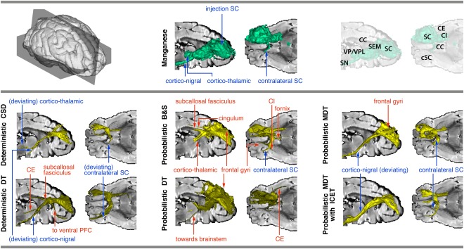
Widespread local connectivity around the injection site was found. Moreover, the tracer visualized the cortico‐nigral tract that terminated in substantia nigra, the cortico‐thalamic tract that terminated in the medial‐dorsal (MD) nucleus, and a cortico‐cortical tract that propagated through the genu of the corpus callosum before terminating in the contralateral cPFC. See Figure 3 (top panel).
Figure 3.
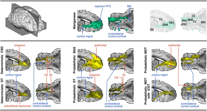
Connectivity of right PFC, reconstructed using manganese tracing (top panel, middle) and tractography (bottom panel). Thresholded tracts are surface‐rendered (for thresholds, see Appendix A1). True positive tracts are labeled in blue, false positive ones in red. For reference, slices of a T2 image are used (right view of a mid‐sagittal slice, and top view of an axial slice through the anterior commissure; see top panel, right). Note that the T2 slices may obscure some of the rendering. Abbreviations: PFC, prefrontal cortex; cPFC, contralateral prefrontal cortex; SEM, centrum semiovale; CC, corpus callosum; SN, substantia nigra; CE, external capsule; MD, medio‐dorsal thalamus; SL, nucleus septalis lateralis; DT, diffusion tensor; CSD, constrained spherical deconvolution; B&S, ball and stick; MDT, multiple diffusion tensor; ICE‐T, iterative confidence enhancement for tractography. [Color figure can be viewed in the online issue, which is available at http://wileyonlinelibrary.com.]
Deterministic tracking
See Figure 3 (bottom panel, left column). Both DT and CSD tractography were able to follow the cortico‐nigral and contralateral cortico‐cortical pathways. However, only CSD was able to follow them for the entire length towards the projection site (cPFC or substantia nigra (SN), respectively). The connection to the MD nucleus of the thalamus, as documented by manganese tracing, could not be found by either method. On the other hand, a number of false positive tracts appeared. Both methods produced false contralateral nucleus septalis lateralis (SL) (branching off from the genu of the corpus callosum at the level of the mid‐sagittal slice) and external capsule (CE) tracts. Also, for CSD a false positive cingulum tract was found that branched off the ipsilateral centrum semiovale (SEM) at the point where the cortico‐nigral and the contralateral cortico‐cortical tracts departed. For the DT, the subcallosal fasciculus (FSC) appeared just on the superior boundary of the caudate, originating from the same point. For both methods, increasing the tractography threshold removed the false positive tracts, but the true pathways could then only be recovered in an incomplete way.
Probabilistic tracking
See Figure 3 (bottom panel, middle and right columns). When using the DT local model, we found the cortico‐nigral and the contralateral cortico‐cortical tract. However, the cortico‐nigral tract ended in WM around the internal capsule area between the caudate and putamen. This may indicate unwanted path length dependency effects. On the other hand, there were false‐positive tracts branching off from the centrum semiovale, following the external capsule and the ipsilateral cingulum. Moreover, we found a false positive tract following the ipsilateral nucleus SL, branching of at the splenium in the mid‐sagittal plane. Increasing the tractography threshold did not ameliorate the situation.
In contrast, the B&S method found, clearly and continuously, the anterior part of the cortico‐nigral tract, as well as the contralateral cortico‐cortical tract toward cPFC. However, in the centrum semiovale, the cortico‐nigral tract suddenly took a different, more dorsal and lateral, route through the internal capsule. Moreover, false positive tracts included the contralateral SL, part of the cingulum and local cortical projections near the injection site. Increasing the tractography threshold removed most false positives, but of the true tracts, only the part of the cortico‐nigral tract anterior to the centrum semiovale remained.
Finally, using the MDT method yielded a somewhat different picture. While the true projections to the contralateral PFC and the substantia nigra were found clearly, many of the false positive tracks found by all the other methods, including the deterministic ones, did not show up, such as the SL, cingulum, subcallosal fasciculum, and external capsule. However, the method did produce a false positive pathway running from the centrum semiovale to the ventro‐medial PFC.
The same method used with the ICE‐T wrapper (threshold 33%) yielded very compact pathways to the true projection sites and showed minimal dependence on path length and threshold. However, this method also produced some false positive tracts, for example, a connection between the centrum semiovale and a more lateral PFC region.
Injection in Motor Cortex
Manganese tracing
The tracers revealed a cortico‐thalamic tract to the ventral‐anterior/ventral‐lateral (VA/VL) nucleus, a cortico‐striatal tract that terminated in caudate nucleus and a cortico‐cortical tract that traversed the mid‐body of corpus callosum and terminated in the contralateral MC. See Figure 4 (top panel).
Figure 4.
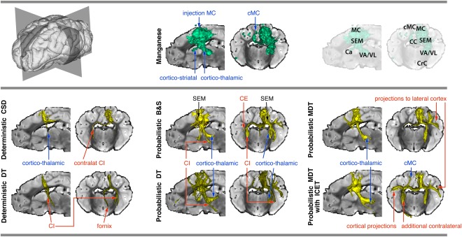
Connectivity of left MC, reconstructed using manganese tracing (top panel, middle) and tractography (bottom panel). Thresholded tracts are surface‐rendered (for thresholds, see Appendix). True positive tracts are labeled in blue, false positive ones in red. For reference, slices of a T2 image are used (left view of a mid‐sagittal slice, and frontal view of a coronal slice through the thalamus; see top panel, right). Note that the T2 slices may obscure some of the rendering. Abbreviations: MC, motor cortex; cMC, contralateral motor cortex; SEM, centrum semiovale; VA/VL, ventro‐anterior/ventro‐lateral thalamus; Ca, anterior commissure; CC, corpus callosum; CE, external capsule; CI, internal capsule; CrC, Crus cerebri; DT, diffusion tensor; CSD, constrained spherical deconvolution; B&S, ball and stick; MDT, multiple diffusion tensor; ICE‐T, iterative confidence enhancement for tractography. [Color figure can be viewed in the online issue, which is available at http://wileyonlinelibrary.com.]
Deterministic tractography
See Figure 4 (bottom panel, left column). Both the CSD and DT variants of deterministic tractography revealed the initial sections of the tracts through the corpus callosum and downward toward the thalamus and caudate, mostly without reaching the actual projection sites (however, CSD did reach the thalamus). These true connections were overshadowed by much more prominent false positive tracts, following the ipsilateral internal capsule pathways, fornix (Fx) and a projection toward PFC (for DT), and the contralateral internal capsule (cCI) (for CSD).
Probabilistic tractography
See Figure 4 (bottom panel, middle and right columns). Both the DT and B&S local models enabled tracking of the pathway to the thalamus (VA/VL region), but not the pathway to the caudate nucleus. False positive tracts include connections projecting toward the brain stem area and to gyri near the injection site. At the given thresholds (see Appendix), DT shows only very weak connections to the contralateral hemisphere (to the MC), while the B&S method crossed the corpus callosum. However, the DT did follow some false‐positive ipsilateral ventral projections within the internal and external capsules that were not visualized by manganese. Lowering the threshold also revealed the contralateral MC connection, but produced false positive projections into many parts of the white matter, originating from the centrum semiovale (both ipsilateral and contralateral) (not shown).
Using the MDT model yielded a similar result as the B&S, but from the contralateral centrum semiovale it did not manage to follow the tract toward the contralateral MC, except at very low thresholds, at which specificity was largely lost. With ICE‐T, the contralateral MC was reached via a relatively wide section of the corpus callosum, which was identical to the one found by manganese tracing. Also, the cortico‐thalamic tract toward VA/VL was mainly correctly reconstructed. However, there are a number of false positive tracts branching off along the pathway. For example, they followed the ipsilateral internal capsule beyond the thalamus and produced another lateral projection. Also, additional lateral and medial projections in the contralateral hemisphere were introduced.
Injection in Somatosensory Cortex
Manganese tracing
The tracer revealed a cortico‐nigral tract that terminated in the substantia nigra, a cortico‐thalamic tract that terminated in the ventral posterior (VP)/ventral posterior lateral (VPL) nucleus, and a cortico‐cortical tract that propagated through the genu of the corpus callosum and terminated in the contralateral SC. See Figure 5 (top panel).
Figure 5.
Connectivity of right SC, reconstructed using manganese tracing (top panel, middle) and tractography (bottom panel). Thresholded tracts are surface‐rendered (for thresholds, see Appendix). True positive tracts are labeled in blue, false positive ones in red. For reference, slices of a T2 image are used (right view of a mid‐sagittal slice, and top view of an axial slice above the anterior commissure; see top panel, right). Note that the T2 slices may obscure some of the rendering. Abbreviations: SC, somatosensory cortex; cSC, contralateral somatosensory cortex; PFC, prefrontal cortex; SEM, centrum semiovale; VA/VL, ventro‐anterior/ventro‐lateral thalamus; CC, corpus callosum; SN, substantia nigra; CE, external capsule; CI, internal capsule; DT, diffusion tensor; CSD, constrained spherical deconvolution; B&S, ball and stick; MDT, multiple diffusion tensor; ICE‐T, iterative confidence enhancement for tractography. [Color figure can be viewed in the online issue, which is available at http://wileyonlinelibrary.com.]
Deterministic tracking
See Figure 5 (bottom panel, left column). For the DT model, tracts projected through the internal capsule, but then turned more inferior and projected toward the brain stem region. The thalamus was not reached. A false positive tract was found, entering the external capsule and following the FSC and a spurious tract from centrum semiovale toward ventral part of PFC. The corpus callosum was crossed more posteriorly compared to the manganese tracing, and the tract reached the contralateral SC but continued (erroneously) into a neighboring gyrus.
The CSD method yielded tracts that projected, via the capsula interna, toward the thalamus, but skirted around VP/VPL and continued toward the brain stem region. Also, some frontally neighboring gyri were reached, which were not obvious in manganese tracing. The corpus callosum was crossed more posteriorly than in the manganese tracing, and the tract reached the contralateral SC (slightly beyond the reach of the manganese tracing). Lowering the threshold did not qualitatively change the connections, but just broadened the tracts.
Probabilistic tracking
See Figure 5 (bottom panel, middle and right columns). For DT, tracts traversed through the internal capsule, after which they curved off along a more inferior route than the manganese, and continued on towards the brain stem region. Additionally, false positive tracts were found going to the external capsule (two paths) and the neighboring gyri (superior and middle frontal gyri). On passing through the corpus callosum, the tracking followed the manganese pathway, but did not cross the corpus callosum to the contralateral hemisphere. When using the B&S model, the centrum semiovale was not traversed over to the internal capsule (as shown by manganese tracing), but instead the tracking followed an alternative, more superior and medial path and terminated at the ventral anterior nucleus of the thalamus. False positive tracts following the subcallosal fasciulus, cingulum, and fornix were also found. Further, ipsilateral cortico‐cortical connections to neighboring frontal gyri were found. Contralateral projections crossed the corpus callosum (posterior to manganese tracing), crossed the contralateral centrum semiovale, skirted around the cSC, and projected toward neighboring ventral gyri and into the internal capsule.
The MDT model resulted in cortico‐nigral tracts reaching the vicinity of the ipsilateral substantia nigra and beyond (but somewhat inferior to the manganese tract) and the contralateral SC (crossing the corpus callosum more dorsally than the manganese tracing). No cortico‐thalamic connection was found. False positive ipsilateral tracts reached the superior frontal gyrus. Using ICE‐T the results were principally the same, but the tracts were more condensed and less spread out, especially near the seed region. Moreover, the tracts were followed for their whole length over a broad range of thresholds. This is supported by the quantitative specificity results in Figure 2.
Variation of Tractography Parameters
Deterministic tensor tracking (MedINRIA)
MedINRIA allows varying the minimum FA for the tracking region, a smoothness parameter controlling the fiber stiffness and the minimum fiber length. We varied these parameters within reasonable limits: smoothness between 0 and 30; fiber length between 5 and 20 mm, FA threshold between 0.1 and 0.15. As expected, the minimum fiber length caused only very minor changes. Variation of the other parameters caused a few isolated effects: (1) injection into prefrontal cortex: increase of the FA threshold to 0.15 caused the cortico‐nigral pathway (Fig. 3) to disappear; (2) injection to motor cortex: decreasing the smoothness to 0 caused another false positive tract in the contralateral internal capsule (the same as for the deterministic CSD tracking, see Fig. 4); (3) injection into somatosensory cortex: increasing the smoothness to 20 or more removed the false positive tract to the ventral PFC (Fig. 5).
Deterministic constrained spherical deconvolution (MRTrix)
The following main parameters may influence the MRTrix streamtrack procedure, when used for deterministic CSD tracking, and were varied (see ranges in brackets): the FA threshold defining the tracking region (0.05–0.15), the minimum curvature radius controlling the fiber stiffness (0–1 mm), the minimum fiber length (5–20 mm), the threshold for the local fODF maximum (0.05–0.2), and the FA threshold for the computation of the deconvolution kernel (0.4–0.8). While the first three of these parameters are also used in tensor tracking, the latter two are specific for spherical deconvolution. The variation of the parameters caused the following effects: (1) injection into prefrontal cortex: while the other parameters had no effect in terms of the presence or absence of pathways, the curvature parameter proved very influential, as the introduction of a minimum curvature radius of 0.5 or 1 mm (i.e., one or two voxels) resulted in an effective suppression of false positive pathways, while the true positive ones remained unaffected; (2) injection to motor cortex: this tractography was somewhat more sensitive towards tracking parameters – minimum curvature constraints caused both true and false tracts to disappear, large minimum length (20 mm) caused more false tracts to appear, and a larger local ODF threshold (0.2) as well as rather low FA thresholds for kernel estimation (<0.6) also caused true and false tracts to disappear; (3) injection into somatosensory cortex: here, only few parameter dependencies were found—for larger minimum curvature (0.5 mm), tracts tended to disappear, and for higher local ODF threshold, the true contralateral SC was reached. Also, FA thresholds below 0.6 removed cortico‐thalamic pathway (which was reconstructed with a deviating pathway for higher thresholds).
Probabilistic tensor tracking (vdconnect, MPI Leipzig)
Varying the FA threshold for tracking from 0.05 to 0.13 (the value used by deterministic tensor and CSD tracking) changed the tracking result only very little, and did not cause any changes with respect to found tracts.
Probabilistic B&S (probtrackx, FSL)
Here we varied the number seed points per voxel (default: 5,000, tested values: 3,000 and 10,000) and the minimum curvature parameters (default 0.2, tested values: 0.1 and 0.3). Both parameters turned out to not influence the result with respect to the found tracts. In addition, the underlying local model employs another important parameter with potential to influence the result: the maximum number of fiber bundles (“sticks”) per voxel. The default is to use maximally two fiber populations per voxel. Increasing this value to 3 caused virtually no change in the results, while reducing it to just 1 had the surprising effect that a number of false positive tracks disappeared, without a notable increase in false negatives.
Probabilistic multi‐tensor (Camino)
The main parameters are the number of streamlines initialised (tested: 3,000, 5,000, 64,000, and 500,000) and the minimum curvature threshold (default 80°, also tested 70° and 90°). While the number of streamlines did not have any visible influence on the result within the tested range (thus, 3,000 streamlines were enough in our case), changing the curvature threshold exercised a slight influence, but did not change the selection of tracts found.
DISCUSSION
Performance of the Algorithms
We evaluated diffusion tractography methods by comparing their results to the ones obtained by manganese tracing. We employed two different modes of comparison. In the “global voxel‐wise comparison,” we studied the overall sensitivity and specificity of each tractography method, as measured in the voxel space, compared to manganese tracing, under the assumption that manganese tracing represents the ground truth. This analysis was designed to reveal, using one single number, to what extent any particular tractography method was capable of characterizing axonal connectivity in a quantitative way. In an additional “qualitative assessment,” we manually assessed the ability of each tractography method to find particular fiber systems that had been revealed by manganese tracing. This analysis was employed to extend the results of the global voxel‐wise comparison in two important ways. First, it allowed for a tract‐specific assessment of the tractography performance and thereby gave cues for the identification of particular weaknesses of the algorithms. Second, this analysis also enabled an assessment at a more conceptual level rather than providing mere voxel agreement. For example, a particular tractography method might follow the same principal pathways and reach the same target areas as manganese tracing, but fails to fill the full volume of the manganese results, thereby decimating voxel‐wise agreement.
The global voxel‐wise comparison revealed that, for all tested tractography methods, it was impossible to reach a high degree of sensitivity (i.e., finding most of the true connections) and specificity (i.e., not finding many false connections) at the same time (i.e., for the same set of thresholds). It was, however, possible to define a range of thresholds for which manganese tracing yielded plausible results, based on the anatomy of the pig brain i.e. [Felix et al., 1999] and histochemical BDAs tracing [Dyrby et al., 2007; Jelsing et al., 2006]. Within that range, it appears that the overall voxel‐wise sensitivity of all tested tractography methods is rather poor. The qualitative assessment revealed that one major reason for this lack of sensitivity is the fact that tractography only follows the central, most coherent part of the tracts, while manganese tracing follows all the axons and thereby produces tract representations with larger cross‐sectional areas. This results in a large number of false negative voxels (i.e. positive in Mn, but negative in tractography). Note, however, that this could also be due to some lack of specificity in the manganese tracing (or the way it is analyzed). See below (section “Study limitations”) for more details on possible caveats of using manganese tracing as a reference for tractography. To a somewhat lesser extent, missing entire tracts (false negatives) and biased trajectories of tracts are also responsible for this loss of sensitivity. Such problems appear to mainly occur after tracts have passed regions with complex fiber arrangements (e.g., the centrum semiovale) or high curvature (e.g., the genu of corpus callosum). The particular choice of tractography method played a significant role in this aspect of performance: clearly algorithms using advanced local models (B&S, CSD, and MDT) were more often able to find the true connections than the DT‐based methods (see Table 1 and Figs. 3, 4, 5). This corroborates conclusions from previous studies, for example, Behrens et al. [2007].
When it comes to specificity, it seems from global voxel‐wise assessment that, within the plausible manganese threshold range, most tractography algorithms perform quite well. However, when a tractography threshold is selected at which all or most major fiber tracts are followed along their whole length, many false positive tracts appear. Hence, even if one does not take into account the compromising of the sensitivity that results from not finding the entire cross‐section area found by the manganese tracts, some inherent incompatibility between sensitivity and specificity remains. Also with respect to specificity, the qualitative assessment revealed considerable performance differences among the tractography methods (see Tab. 1 and Figs. 3, 4, 5). Most notably, the multiple tensor‐based probabilistic tractography implemented in Camino yielded higher specificity (i.e., fewer false tracts) as compared to the rest of the approaches, while the (single) tensor based approaches, and also the B&S method, produced many false positives. As already found for the sensitivity problems, the origin of many of the false tracts seem to lie in regions with complex fiber architecture, such as the centrum semiovale. Apparently, the ability of many of the employed local models to account for fiber crossings was not sufficient for the correct identification of tracts.
The postprocessing using ICE‐T led to some gain in sensitivity (contralateral MC was reached), but also to some loss in specificity (some false contralateral connections with the MC injection site). The method appears to promote very concentrated tracts that do not always overlap precisely with the manganese tracts. Moreover, the performance of the method is relatively independent of the threshold and the path length. Path length dependency is a property of the most current tractography schemes, both deterministic and probabilistic, resulting from the iterative nature of the algorithms and the consequent error accumulation [for a discussion, see Li et al., 2012]. It causes larger spread and lower streamline counts for more distant targets. Note, however, that there also can be a path length dependency in the underlying ground truth, as more and more axons branch off from a major tract the further one moves away from a seed area. This effect is a complex phenomenon that varies, for example, between brain areas [Markova et al., 2013]. It has been demonstrated experimentally using tracer experiment [Ercsey‐Ravasz et al., 2013; Markova et al., 2013]. Also, in our manganese tracing results, there is a clear interaction between SNR (as reflected by the threshold) and distance from the injection area (see Fig. 1). So, when using ICE‐T, one should bear in mind that besides the artifactual path length dependency also the natural one might get eliminated.
Influence of Tractography Parameters
Although it was not within the scope of this work to perform a full‐fledged parameter study of the investigated tractography algorithms, the parameter variations that we did perform suggest that some of the parameters have an impact onto the number of tracts found, but do not really distinguish between true and false tracts. In other words, a parameter change that lets false positive tracts disappear also tends to remove true positives (e.g., minimum curvature in deterministic CSD tracking). An exception is the maximum number of fiber bundles per voxel in the B&S algorithm, where, in our examples, using just one fiber bundle consistently yielded fewer false positives than using two or three bundles. This result is somewhat surprising in the light of previous findings. After all, it is well established that with usual image resolutions a large proportion of the voxels in the brain contain more than one fiber population [Behrens et al., 2007; Jeurissen et al., 2013], and, therefore, assuming just a single direction per voxel should lead to missing tracts (i.e., false negatives), as demonstrated impressively by Behrens et al. [2007]. However, our results demonstrate that this has also a downside, as, at least in the tested configurations, false positive tracts can be generated. This problem might be rooted in insufficient image resolution, because even with sophisticated fiber orientation models crossing, it is very difficult to distinguish between bending and “kissing” of fiber populations within one voxel [see, e.g., Jones et al., 2012].
Of course, there are potentially many more algorithmic choices that might have a profound influence on the performance of tractography algorithms. A rigorous evaluation of these would be of great interest, but requires the implementation of a generic framework within which all the algorithms can be placed. One potentially important factor is the seeding strategy. Here, we follow the current practice that probabilistic tractography is usually seeded only in the area of interest (local seeding), while deterministic tractography is mostly seeded in the entire brain with subsequent selection of the fibers by means of an inclusion region (global seeding). However, a systematic influence of the seeding strategy onto the tractography results is to be expected, as global seeding emphasizes connections that involve large and long tracts, while local seeding yields larger connectivity values for short tracts. A systematic evaluation of these effects, using the same (probabilistic) tractography method, has been performed by Li et al. [2012]. When comparing ex vivo tracking in macaque brains with the previous tracer results none of the tested seeding strategies was clearly superior. On the other hand, when deriving graph based measures (small‐world indices, hubs, and hemispheric asymmetries) from the tractography results, substantial differences between seeding methods were observed. As stated by these authors more work on the effect of seeding strategies, also involving more different tractography methods, is needed.
Significance of Results and Possible Ways Forward
In summary, both global voxel‐wise comparison and qualitative assessment revealed that, for all tested tractography methods, reaching a high degree of sensitivity (i.e., finding all true tracts) and specificity (i.e., not finding false tracts) at the same time is difficult or impossible. Such problems have been known since the advent of diffusion tractography. As a major consequence, researchers have developed a whole range of sophisticated methods, in particular those for modeling the local fiber configuration within a voxel [Seunarine and Alexander, 2009]. In fact, our results confirm that these efforts have been at least partially fruitful. However, it is also evident that none of the methods performed without errors and that all the local models seem to have similar problems, even if they are able to accommodate crossing fiber configurations. We do not conclude from this that the more realistic local models have no benefit for tractography [Behrens et al., 2007], but simply that their power is not sufficient for the challenges posed in this specific case. However, our results are strikingly in line with a recent study of Thomas and colleagues [2014], who used high‐resolution ex vivo tractography of macaque in comparison with atlas data from tracer studies to assess the accuracy of various methods. They also reach the conclusion that gains in sensitivity are generally achieved by loss in specificity and vice versa. This is all the more remarkable, as in our study we are using a quite different set of techniques to assess (partially) the same set of tractography methods: (1) we use a within‐subject comparison rather that a comparison with atlas data; (2) we use voxel‐wise and qualitative tract‐wise, rather that region‐wise, comparison.
At first glance somewhat in contrast to these and our results are the findings of Jbabdi et al. [2013], who reported good agreement between in vivo tracer and B&S tractography results in macaques. While in their data the voxel‐wise agreement between tracing and tractography seems also quite limited (as it appears from the figures), the qualitative agreement is remarkable. They used a technique that has not been used here, namely the use of inclusion and exclusion masks. This is a very potent way of incorporating prior assumptions into the tracking procedure and of course reduces the chance for false positives dramatically.
It should be noted that a certain incompatibility between sensitivity and specificity is a general property of every attempt to reconstruct the underlying sources from noisy and undersampled data (see below). With given data, at some point trying to reveal even more detail from the data (by using more complex models with more degrees of freedom) goes along with the risk of interpreting noise and generating false positives. So, it is important to state that our results also show that with current methods and data it is quite possible to make valid (i.e., highly specific) reconstructions, albeit at the cost of some loss in sensitivity.
Our findings suggest that the observed performance problems are not solely due to the constraints imposed by the local models and the type of employed tractography, but they are also a consequence of the limited amount of available data. In fact, the estimation of the diffusion propagator (i.e., the particle displacement distribution function) is subject to subsampling in four dimensions [Jones et al., 2012]: spatial, angular, diffusion time, and diffusion length (displacement of molecules). In practice, each of these factors is severely undersampled: voxels are so big that they contain multiple fiber populations; commonly used angular resolution (e.g., 60 directions) allows for reconstruction of fiber bundles separated no less than 30–45° [Descoteaux et al., 2009]; and using just one or a few (and often rather low) b‐values limits the angular resolution between parallel‐oriented barriers, such as axonal membranes [Descoteaux et al., 2009; Dyrby et al., 2011]. The relative importance of these factors is a matter of ongoing debate. However, our experience with the application of high angular resolution local models in complex regions (e.g., the centrum semiovale) suggests that the main source of deficiency is the lack of sufficient spatial (voxel) resolution, leading to partial volume effects (PVE). However, also a lack of angular resolution, mainly caused by small b‐values, may play an important role. As a consequence, we argue that, while there are certainly benefits of using sophisticated local models and tracking strategies, they will only have a chance to be fully effective once this data deficiency has been overcome (minimal PVE). A major obstacle on the road to better spatial and angular resolution is scanning time—particularly within clinical settings. One of the most successful ways of accelerating multiple slice acquisitions is multiband imaging [Moeller et al., 2010; Setsompop et al., 2012]. Another promising improvement in that respect is the recent development of multiplexing [Feinberg et al., 2010; Reese et al., 2009], along with compressed sensing [Doneva et al., 2010; Landman et al., 2011; Landman et al., 2010; Menzel et al., 2011; Michailovich and Rathi, 2010; Michailovich et al., 2011]. Stronger gradients in clinical scanners play a key role for ensuring improved SNR (via minimizing TE), higher b‐values, as well as contrast to microstructural details [Dyrby et al., 2013]. Also, the use of high static magnetic fields in combination with parallel imaging and reduced field‐of‐view has been shown to improve the SNR and allow for superior voxel resolution [Heidemann et al., 2011; Heidemann et al., 2010]. Substantial advances towards higher SNR, faster scanning and improved resolution have been achieved by the Human Connectome Project [for overviews, see Setsompop et al., 2013; Sotiropoulos et al., 2013].
Alternatively, tractography algorithms might profit from the incorporation of additional knowledge of the fiber tracts to be reconstructed. We know, for example, that DWI datasets contain a high degree of spatial coherence, due to extended bundles of projecting axon, and tractography might still not use the full potential of this information. Dyrby et al. [2014] show that interpolating either the raw diffusion MRI data or the reconstructed local model (e.g., the DT) potentially enables the extraction of finer anatomical details that are normally seen only at the higher image resolution. The authors argue that the anisotropic spatial coherence is likely to be the underlying source of this additional information. Similarly, “Track Density Imaging” by Calamante et al. [2010] uses, instead of interpolated raw data, the streamlines as “'spatial interpolators” at a very high image resolution and can map fine anatomical structures that were not visible at original image resolution. Rowe et al. [2012] use anatomical knowledge on how fiber tracts can disperse at the front‐end of the tracking and demonstrate promising new features and robustness in tracking . Finally, the use of inclusion/exclusion maps is an effective means of eliminating many a priori senseless tracts [Jbabdi et al., 2013].
Study Limitations
There are a number of potential caveats for the universality of the above conclusions. First, it has to be made clear that manganese tracing does not necessarily represent the absolute truth in terms of fiber architecture: Manganese tracing also has a limited image resolution, leading to a considerable incidence of PVE, especially in narrow passages such as the tracts to the substantia nigra and the thalamus. There is also a substantial intercellular spread of manganese around the injection site, creating a large diffuse region of false positives. This also causes some uncertainty about exactly which axons take up the manganese. Possibly a similar, but less prominent, extracellular diffusion effect also occurs at the projections sites where transported manganese is accumulated. This unspecific spreading forces higher thresholds, which in turn leads to reduced detectability of the actual fiber tracts. Also, if following a number of axons originating at the injection site, the branching‐off of more and more axons may lead to a general path length dependency of tracer results [Ercsey‐Ravasz et al., 2013; Markova et al., 2013]. As a consequence, the aforementioned imperfections of manganese tracing may lead to systematic false negatives at the far ends of the tracts, that is, tracts do not appear to reach their final destination in gray matter.
A second issue in this study is that in order to be able to use the ground truth information provided by invasive tracing, we used mini pig brains. This leads to a potential problem in the applicability of the results to humans. In order to minimize this problem, the imaging parameters, e.g., voxel size, were chosen such that they were equivalent to commonly used image resolution in human experiments. Also, the chosen b‐value was adapted to the ex vivo situation and corresponded closely to a clinical in vivo experiment [Dyrby et al. 2011]. However, due to the strongly non‐linear relationship between the white matter fiber architectures in pigs and humans, this compatibility cannot be perfect. For example, pig brains have, in relation to their size, much thinner white matter than humans [Lind et al., 2007]. This may render the effective image resolution in pigs coarser than that in humans and explain some of the difficulties tractography has in complex regions like the centrum semiovale. On the other hand, in terms of image quality (artefacts, SNR, motion) the present data are significantly better than average clinical human data. Therefore, the observed problems are most likely to also be present in human experiments, at least partially.
Another potential caveat to the analysis provided here lies in the co‐registration between in vivo manganese tracing and ex vivo diffusion MRI, as well as between different pig brains. In order to assess the quality of the registration, we matched visible landmarks in the manganese images (i.e., projection sites) with their known anatomical counterparts in the diffusion MRI data. We found an agreement on the order of the size of a single voxel. Therefore, and considering the spatial extent of the tracts, it is not likely that co‐registration problems explain a major part of our results.
Also, the suggestion that higher spatial resolution might be the road to success in improving the situation seems to be partially at odds with the findings of Thomas and colleagues [2014], who detected similar problems at half the voxel size we used (with roughly similar brain size between macaque and mini pig). The question remains whether this can be interpreted as general proof that better voxel resolution will not solve the problem, or whether their voxel resolution of 0.25 mm is still too coarse. However, a direct quantitative comparison between their and our results is not possible because of the strongly different assessment techniques.
Finally, the study is limited by the fact that we were not able to test all known tractography methods. Herein we have chosen a range of popular methods spanning most major classes of techniques. We, therefore, believe that the problems found are not solvable by better algorithms alone.
It is clear from the above considerations that manganese tracing alone, in spite of its undisputed merits (that have motivated us to use it in the first place), does not provide a “gold standard” for axonal connections, but only a “silver standard.” Many independent methods for validation of tractography already exist, but they all have their advantages and drawbacks. Among the tracer methods, manganese is important, because it can be globally imaged in the intact brain and thereby easily compared with tractography results. Unfortunately, this advantage is inherently linked to some major limitations (related to, e.g., MRI voxel size and SNR), so cross‐validation with alternative methods is needed (as also done in this study). In the future, validation approaches might therefore use a kind of “committee strategy,” where several independent (typically invasive and some of them tissue destructive) methods are combined for providing a more complete picture of the challenges and possibilities that tractography methods face in in vivo brain tissue. Such a committee validation strategy could combine different types of invasive tracers [Innocenti et al., 2013; Jelsing et al., 2006; Markov et al., 2014; Schmahmann et al., 2007], for knowing the exact projections from particular starting regions (connection oriented approach), with polarized light imaging [Caspers et al., 2015] and structure tensor analysis [Budde and Annese, 2013], for providing high‐resolution accounts of the orientational structure of the tissue and the spatial relationships between fiber populations (volume oriented approach). For cross‐validation, also microscopic myelin imaging together with optical clearing methods (e.g., with clear lipid‐exchanged acrylamide‐hybridized rigid imaging) [see, e.g., Spence et al., 2014] might play an important role. While the above techniques can be applied in laboratory animals or postmortem samples, and therefore their results are fairly realistic with respect to the domains of practical application of tractography (mostly in vivo human), physical phantoms are much more of an abstraction of reality. On the other hand, they do provide a real ground truth. Certainly, the comparative evaluation of tractography methods with the help of phantoms [Fillard et al., 2011; Neher et al., 2013; Schreiber et al., 2014] can deliver important insights into the specific strengths and weaknesses of the methods. However, it must be born in mind that the results of such a comparison might be biased by the degree to which the tested methods conform with the particular simplifications embodied in the phantom, for example the parallelism of the fibers or the specific way of interdigitation at crossings. It is, therefore, quite possible that those techniques that perform well in a certain type of phantom do not so in the real brain.
CONCLUSIONS
In this study, a representative selection of tractography methods was evaluated by comparing them with invasive manganese tracing. We found that, in general, tractography methods were capable of finding the major fiber tracts, with some important performance differences existing between the methods, thus confirming the benefit of using some of the more sophisticated approaches. With moderate thresholds and therefore limited sensitivity (i.e., some tracts are missed) specificity can be kept high and results are valid (with no or few false positives). However, we also discovered that at higher thresholds false positive connections were very common, and it is difficult to achieve high sensitivity (i.e., few false negatives) and high specificity (i.e., few false positives) at the same time. We observed that these problems mainly originate from regions with complex fiber arrangements or high curvature and are not easily resolved by sophisticated local models alone. Instead, the crucial challenge in making tractography a truly useful and reliable tool in brain research and neurology lies in the acquisition of better data. In particular, we hypothesize that the increase of spatial resolution, whilst preserving the SNR, is the key. The validity of this assumption remains to be investigated in future studies.
ACKNOWLEDGMENTS
The study was a part of the EU FP7 project CONNECT (consortium of neuroimagers for the non‐invasive exploration of brain connectivity and tracts). None of the authors have any conflict of interest to declare with the subject matter.
THRESHOLD VALUES FOR QUALITATIVE COMPARISON
The thresholds for tracing and tracking shown in Table 2 were manually chosen to optimize the balance between specificity and sensitivity. They are expressed as percentage of the maximum value.
Table 2.
Thresholds for tracing and tracking
| % | injection PFC | Injection MC | Injection SC |
|---|---|---|---|
| Manganese tracing | 25 | 20 | 35 |
| Deterministic DT | 12.5 | 12.5 | 5 |
| Deterministic CSD | 10 | 10 | 10 |
| Probabilistic DT | 60 | 50 | 55 |
| Probabilistic B&S | 1 | 1 | 1 |
| Probabilistic MDT | 1 | 1 | 1 |
| Probabilistic MDT with ICE‐T | 33 | 5 | 10 |
PFC, prefrontal cortex; MC, motor cortex; SC, somatosensory cortex; DT, diffusion tensor; CSD, constrained spherical deconvolution; B&S, ball and stick; MDT, multiple DT; and ICE‐T, iterative confidence enhancement for tractography.
REFERENCES
- Aganj I, Lenglet C, Sapiro E, Yacoub E, Ugurbil K, Harel N (2010): Reconstruction of the orientation distribution function in single and multiple shell q‐abll imaging with constant solid angle. Magn Reson Med 64:554–566. [DOI] [PMC free article] [PubMed] [Google Scholar]
- Alexander DC (2005a): Multiple‐fiber reconstruction algorithms for diffusion MRI. Ann N Y Acad Sci 1064:113–133. [DOI] [PubMed] [Google Scholar]
- Alexander DC (2005b): Maximum entropy spherical deconvolution for diffusion MRI. Inf Process Med Imaging 19:76–87. [DOI] [PubMed] [Google Scholar]
- Alexander DC, Barker GJ, Arridge SR (2002): Detection and modeling of non‐Gaussian apparent diffusion coefficient profiles in human brain data. Magn Reson Med 48:331–340. [DOI] [PubMed] [Google Scholar]
- Anwander A, Tittgemeyer M, von Cramon DY, Friederici AD, Knösche TR (2007): Connectivity‐based parcellation of Broca's area. Cereb Cortex 17:816–825. [DOI] [PubMed] [Google Scholar]
- Basser PJ, Mattiello J, LeBihan D (1994): Estimation of the effective self‐diffusion tensor from the NMR spin echo. J Magn Reson B 103:247–254. [DOI] [PubMed] [Google Scholar]
- Behrens TE, Woolrich MW, Jenkinson M, Johansen‐Berg H, Nunes RG, Clare S, Matthews PM, Brady JM, Smith SM (2003): Characterization and propagation of uncertainty in diffusion‐weighted MR imaging. Magn Reson Med 50:1077–1088. [DOI] [PubMed] [Google Scholar]
- Behrens TEJ, Berg HJ, Jbabdi S, Rushworth MFS, Woolrich MW (2007): Probabilistic diffusion tractography with multiple fibre orientations: What can we gain? NeuroImage 34:144–155. [DOI] [PMC free article] [PubMed] [Google Scholar]
- Budde MD, Annese J (2013): Quantification of anisotropy and fiber orientation in human brain histological sections. Front Integr Neurosci 7:3 [DOI] [PMC free article] [PubMed] [Google Scholar]
- Calamante F, Tournier J, Jackson G, Connelly A (2010): Track‐density imaging (TDI): Super‐resolution white matter imaging using whole‐brain track‐density mapping. NeuroImage 53:1233–1243. [DOI] [PubMed] [Google Scholar]
- Caspers S, Axer M, Caspers J, Jockwitz C, Jütten K, Reckfort J, Grässel D, Amunts K, Zilles K (2015): Target sites for transcallosal fibers in human visual cortex ‐ A combined diffusion and polarized light imaging study. Cortex. pii: S0010‐9452(15)00030‐1. [DOI] [PubMed] [Google Scholar]
- Conturo TE, Lori NF, Cull TS, Akbudak E, Snyder AZ, Shimony JS, McKinstry RC, Burton H, Raichle ME (1999): Tracking neuronal fiber pathways in the living human brain. Proc Natl Acad Sci USA 96:10422–10427. [DOI] [PMC free article] [PubMed] [Google Scholar]
- Cook PA, Bai Y, Nedjati‐Gilani S, Seunarine KK, Hall MG, Parker GJ, Alexander DC (2006): Camino: Open‐source diffusion‐MRI reconstruction and processing. Proc Intl Soc Magn Reason Med 14:2759. [Google Scholar]
- D'Arceuil HE, Westmoreland S, de Crespigny AJ (2007): An approach to high resolution diffusion tensor imaging in fixed primate brain. Neuroimage 35:553–565. [DOI] [PubMed] [Google Scholar]
- Dauguet J, Peled S, Berezovskii V, Delzescaux T, Warfield SK, Born R, Westin CF (2007): Comparison of fiber tracts derived from in‐vivo DTI tractography with 3D histological neural tract tracer reconstruction on a macaque brain. NeuroImage 37:530–538. [DOI] [PubMed] [Google Scholar]
- Dell'Acqua F, Scifo P, Rizzo G, Catani M, Simmons A, Scotti G, Fazio F (2010): A modified damped Richardson‐Lucy algorithm to reduce isotropic background effects in spherical deconvolution. NeuroImage 49:1446–1458. [DOI] [PubMed] [Google Scholar]
- Descoteaux M, Angelino E, Fitzgibbons S, Deriche R (2007): Regularized, fast, and robust analytical Q‐Ball imaging. Magn Reson Med 58:497–510. [DOI] [PubMed] [Google Scholar]
- Descoteaux M, Deriche R, Knösche TR, Anwander A (2009): Deterministic and probabilistic tractography based on complex fibre orientation distributions. IEEE Trans Med Imaging 28:269–286. [DOI] [PubMed] [Google Scholar]
- Doneva M, Boernert P, Eggers H, Stehning C, Senegas J, Mertins A (2010): Compressed sensing reconstruction for magnetic resonance parameter mapping. Magn Reson Med 64:1114–1120. [DOI] [PubMed] [Google Scholar]
- Dyrby T, Lundell H, Burke M, Reislev N, Paulson O, Ptito M, Siebner H (2014): Interpolation of diffusion weighted imaging datasets. NeuroImage 103:202–213. [DOI] [PubMed] [Google Scholar]
- Dyrby T, Søgaard L, Hall M, Ptito M, Alexander D (2013): Contrast and stability of the axon diameter index from microstructure imaging with diffusion MRI. Magn Reson Med 70:711–721. [DOI] [PMC free article] [PubMed] [Google Scholar]
- Dyrby TB, Baare WFC, Alexander DC, Jelsing J, Garde E, Sogaard LV (2011): An ex vivo imaging pipeline for producing high‐quality and high‐resolution diffusion‐weighted imaging datasets. Hum Brain Mapp 32:544–563. [DOI] [PMC free article] [PubMed] [Google Scholar]
- Dyrby TB, Sogaard LV, Parker GJ, Alexander DC, Lind NM, Baare WFC, Hay‐Schmidt A, Eriksen N, Pakkenberg B, Paulson OB, Jelsing J (2007): Validation of in vitro probabilistic tractography. NeuroImage 37:1267–1277. [DOI] [PubMed] [Google Scholar]
- Ercsey‐Ravasz M, Markov NT, Lamy C, Van Essen DC, Knoblauch K, Toroczkai Z, Kennedy H (2013): A predictive network model of cerebral cortical connectivity based on a distance rule. Neuron 80:184–197. [DOI] [PMC free article] [PubMed] [Google Scholar]
- Feinberg DA, Moeller S, Smith SM, Auerbach E, Ramanna S, Glasser MF, Miller KL, Ugurbil K, Yacoub E (2010): Multiplexed echo planar imaging for sub‐second whole brain fmri and fast diffusion imaging. Plos One 5:e15710. [DOI] [PMC free article] [PubMed] [Google Scholar]
- Felix B, Léger EM, Albe‐Fessard D, Marcilloux JC, Rampin O, Laplace JP, Duclos A, Fort F, Gougis S, Costa M, Duclos N (1999): Stereotaxic atlas of the pig brain. Brain Res Bull 49:1–137. [DOI] [PubMed] [Google Scholar]
- Fillard P, Descoteaux M, Goh A, Gouttard S, Jeurissen B, Malcolm J, Ramirez‐Manzanares A, Reisert M, Sakaie K, Tensaouti F, Yo T, Mangin JF, Poupon C (2011): Quantitative evaluation of 10 tractography algorithms on a realistic diffusion MR phantom. Neuroimage 56:220–234. [DOI] [PubMed] [Google Scholar]
- Gutman DA, Magnuson M, Majeed W, Keifer OP, Jr. , Davis M, Ressler KJ, Keilholz S (2013): Mapping of the mouse olfactory system with manganese‐enhanced magnetic resonance imaging and diffusion tensor imaging. Brain Struct Funct 218:527–537. [DOI] [PMC free article] [PubMed] [Google Scholar]
- Heidemann R, Anwander A, Feiweier T, Grinstead J, Lohmann G, Knösche T, Turner R (2011): k‐space and q‐space: combining ultra‐high spatial and angular resolution in diffusion imaging using ZOOPPA at 7T. Proc Intl Soc Magn Reson Med 19:1957. [Google Scholar]
- Heidemann RM, Porter DA, Anwander A, Feiweier T, Heberlein K, Knösche TR, Turner R (2010): Diffusion imaging in humans at 7T using readout‐segmented EPI and GRAPPA. Magn Reson Med 64:9–14. [DOI] [PubMed] [Google Scholar]
- Innocenti GM, Vercelli A, Caminiti R (2013): The diameter of cortical axons depends both on the area of origin and target. Cereb Cortex 24:2178–2188. 2013. [DOI] [PubMed] [Google Scholar]
- Jbabdi S, Lehman JF, Haber SN, Behrens TE (2013): Human and monkey ventral prefrontal fibers use the same organizational principles to reach their targets: Tracing versus tractography. J Neurosci 33:3190–3201. [DOI] [PMC free article] [PubMed] [Google Scholar]
- Jelsing J, Hay‐Schmidt A, Dyrby T, Hemmingsen R, Uylings HB, Pakkenberg B (2006): The prefrontal cortex in the Gottingen minipig brain defined by neural projection criteria and cytoarchitecture. Brain Res Bull 70:322–336. [DOI] [PubMed] [Google Scholar]
- Jeurissen B, Leemans A, Tournier JD, Jones DK, Sijbers J (2013): Investigating the prevalence of complex fiber configurations in white matter tissue with diffusion magnetic resonance imaging. Hum Brain Mapp 34:2747–2766. [DOI] [PMC free article] [PubMed] [Google Scholar]
- Jones D (2010): Challenges and limitations of quantifying connectivity in the human brain in vivo with diffusion MRI. Imaging Med 2:341–355. [Google Scholar]
- Jones DK, Cercignani M (2010): Twenty‐five pitfalls in the analysis of diffusion MRI data. NMR Biomed 23:803–820. [DOI] [PubMed] [Google Scholar]
- Jones DK, Knösche TR, Turner R (2013): White matter integrity, fiber count, and other fallacies: The do's and don'ts of diffusion MRI. NeuroImage 73:239–254. [DOI] [PubMed] [Google Scholar]
- Jones DK, Pierpaoli C (2005): Confidence mapping in diffusion tensor magnetic resonance imaging tractography using a bootstrap approach. Magn Reson Med 53:1143–1149. [DOI] [PubMed] [Google Scholar]
- Kaden E, Knösche TR, Anwander A (2007): Parametric spherical deconvolution: Inferring anatomical connectivity using diffusion MR imaging. NeuroImage 37:474–488. [DOI] [PubMed] [Google Scholar]
- Koch MA, Norris DG, Hund‐Georgiadis M (2002): An investigation of functional and anatomical connectivity using magnetic resonance imaging. NeuroImage 16:241–250. [DOI] [PubMed] [Google Scholar]
- Landman B, Bogovic J, Wan H, ElShahaby FEZ, Bazin P‐L, Prince JL (2012): Resolution of crossing fibers with constrained compressed sensing using diffusion tensor MRI. NeuroImage 59:2175–2186. [DOI] [PMC free article] [PubMed] [Google Scholar]
- Landman BA, Wan H, Bogovic JA, Bazin P‐L, Prince JL (2010): Resolution of crossing fibers with constrained compressed sensing using traditional diffusion tensor MRI. Proc SPIE Int Soc Opt Eng. 7623:76231H. [DOI] [PMC free article] [PubMed] [Google Scholar]
- Lazar M, Weinstein DM, Tsuruda JS, Hasan KM, Arfanakis K, Meyerand ME, Badie B, Rowley HA, Haughton V, Field A, Alexander AL (2003): White matter tractography using diffusion tensor deflection. Hum Brain Mapp 18:306–321. [DOI] [PMC free article] [PubMed] [Google Scholar]
- Li L, Rilling JK, Preuss TM, Glasser MF, Hu X (2012): The effects of connection reconstruction method on the interregional connectivity of brain networks via diffusion tractography. Hum Brain Mapp 33:1894–1913. [DOI] [PMC free article] [PubMed] [Google Scholar]
- Lin CP, Tseng WYI, Cheng HC, Chen JH (2001): Validation of Diffusion Tensor Magnetic Resonance Axonal Fiber Imaging with Registered Manganese‐Enhanced Optic Tracts. NeuroImage 14:1035–1047. [DOI] [PubMed] [Google Scholar]
- Lind NM, Moustgaard A, Jelsing J, Vajta G, Cumming P, Hansen AK (2007): The use of pigs in neuroscience: Modeling brain disorders. Neurosci Biobehav Rev 31:728–751. [DOI] [PubMed] [Google Scholar]
- Liptrot G, Sidaros K, Dyrby T (2014): Addressing the path‐length‐dependency confound in white matter tract segmentation. Plos One 9:e96247. [DOI] [PMC free article] [PubMed] [Google Scholar]
- Liu C, Bammer R, Acar B, Moseley M (2004): Characterizing non‐Gaussian diffusion by using generalized diffusion tensors. Magn Reson Med 51:924–937. [DOI] [PubMed] [Google Scholar]
- Markov NT, Ercsey‐Ravasz MM, Gomes ARR, Lamy C, Magrou L, Vezoli J, Misery P, Falchier A, Quilodran R, Gariel MA, Sallet J, Gamanut R, Huissoud C, Clavagnier S, Giroud P, Sappey‐Marinier D, Barone P, Dehay C, Toroczkai Z, Knoblauch K, Van Essen DC, Kennedy H (2014): A weighted and directed interareal connectivity matrix for macaque cerebral cortex. Cerebral Cortex 24:17–36. [DOI] [PMC free article] [PubMed] [Google Scholar]
- Markova, N.T , Ercsey‐Ravasz, M , Lamy, C , Gomes, A.R.R , Magrou, L , Misery, P , Giroud, P , Barone, P , Dehay, C , Toroczkai, Z , Knoblauch, K , Van Essen, D.C , Kennedy, H , 2013. The role of long‐range connections on the specificity of the macaque interareal cortical network. Proc Natl Acad Sci USA 110:5187–5192. [DOI] [PMC free article] [PubMed] [Google Scholar]
- Menzel MI, Tan ET, Khare K, Sperl JI, King KF, Tao X, Hardy CJ, Marinelli L (2011): Accelerated diffusion spectrum imaging in the human brain using compressed sensing. Magn Reson Med 66:1226–1233. [DOI] [PubMed] [Google Scholar]
- Michailovich O, Rathi Y (2010): Fast and accurate reconstruction of HARDI data using compressed sensing. Med Image Comput Comput Assist Interv 2010;13(Pt 1):607–614. [DOI] [PMC free article] [PubMed] [Google Scholar]
- Michailovich O, Rathi Y, Dolui S (2011): Spatially regularized compressed sensing for high angular resolution diffusion imaging. IEEE Trans Med Imaging 30:1100–1115. [DOI] [PMC free article] [PubMed] [Google Scholar]
- Moeller S, Yacoub E, Olman CA, Auerbach E, Strupp J, Harel N, Ugurbil K (2010): Multiband multislice GE‐EPI at 7 tesla, with 16‐fold acceleration using partial parallel imaging with application to high spatial and temporal whole‐brain fMRI. Magn Reson Med 1144–1153. [DOI] [PMC free article] [PubMed] [Google Scholar]
- Mori S, Crain BJ, Chacko VP, van Zijl PCM (1999): Three‐dimensional tracking of axonal projections in the brain by magnetic resonance imaging. Ann Neurol 45:265–269. [DOI] [PubMed] [Google Scholar]
- Mori S van Zijl PC, 2002. Fiber tracking: principles and strategies ‐ A technical review. NMR Biomed 15:468–480. [DOI] [PubMed] [Google Scholar]
- Neher PF, Laun FB, Stieltjes B, Maier‐Hein KH 2013. Fiberfox: Facilitating the creation of realistic white matter software phantoms. Magn Reson Med 72:1460–1470. [DOI] [PubMed] [Google Scholar]
- Patel V, Shi Y, Thompson PM, Toga AW (2010): Mesh‐based spherical deconvolution: A flexible approach to reconstruction of non‐negative fiber orientation distributions. NeuroImage 51:1071–1081. [DOI] [PMC free article] [PubMed] [Google Scholar]
- Reese TG, Benner T, Wang R, Feinberg DA, Wedeen VJ (2009): Halving imaging time of whole brain diffusion spectrum imaging and diffusion tractography using simultaneous image refocusing in EPI. J Magn Reson Imaging 29:517–522. [DOI] [PMC free article] [PubMed] [Google Scholar]
- Riffert TW, Schreiber J, Anwander A, Knösche TR (2014): Beyond fractional anisotropy: Extraction of bundle‐specific structural metrics from crossing fiber models. Neuroimage 100:176–191. [DOI] [PubMed] [Google Scholar]
- Rowe M, Zhang H, Alexander D (2012): Utilising measures of fiber dispersion in white matter tractography. MICCAI Workshop on Computational Diffusion MRI, Nice. pp. 2–12. [Google Scholar]
- Schmahmann JD, Pandya DN, Wang R, Dai G, D'Arceuil HE, de Crespigny AJ, Wedeen VJ (2007): Association fibre pathways of the brain: Parallel observations from diffusion spectrum imaging and autoradiography. Brain 130:630–653. [DOI] [PubMed] [Google Scholar]
- Schreiber J, Riffert T, Anwander A, Knösche TR (2014): Plausibility tracking: A method to evaluate anatomical connectivity and microstructural properties along fiber pathways. Neuroimage 90:163–178. [DOI] [PubMed] [Google Scholar]
- Setsompop K, Gagoski BA, Polimeni JR, Witzel T, Wedeen VJ, Wald LL (2012): Blipped‐controlled aliasing in parallel imaging for simultaneous multislice echo planar imaging with reduced g‐factor penalty. Magn Reson Med 1210–1224. p [DOI] [PMC free article] [PubMed] [Google Scholar]
- Setsompop K, Kimmlingen R, Eberlein E, Witzel T, Cohen‐Adad J, McNab JA, Keil B, Tisdall MD, Hoecht P, Dietz P, Cauley SF, Tountcheva V, Matschl V, Lenz VH, Heberlein K, Potthast A, Thein H, Van Horn J, Toga A, Schmitt F, Lehne D, Rosen BR, Wedeen V, Wald LL (2013): Pushing the limits of in vivo diffusion MRI for the Human Connectome Project. Neuroimage 220–233. p [DOI] [PMC free article] [PubMed] [Google Scholar]
- Seunarine, K.K , Alexander, D.C , 2009. Multiple fibres: beyond the diffusion tensor In: Johansen‐Berg H, Behrens TE, editors. Diffusion MRI, from Quantitative Measurement to In‐Vivo Neuroanatomy. Academic Press, San Diego, 55–72. [Google Scholar]
- Sotiropoulos SN, Jbabdi S, Xu J, Andersson JL, Moeller S, Auerbach EJ, Glasser MF, Hernandez M, Sapiro G, Jenkinson M, Feinberg DA, Yacoub E, Lenglet C, Van Essen DC, Ugurbil K, Behrens TEJ, Consortium WMH (2013): Advances in diffusion MRI acquisition and processing in the Human Connectome Project. Neuroimage 125–143. [DOI] [PMC free article] [PubMed] [Google Scholar]
- Spence RD, Kurth F, Itoh N, Mongerson CRL, Wailes SH, Peng MS, MacKenzie‐Graham AJ (2014): Bringing CLARITY to gray matter atrophy. Neuroimage 101:625–632. [DOI] [PMC free article] [PubMed] [Google Scholar]
- Sun SW, Neil JJ, Liang HF, He YY, Schmidt RE, Hsu CY, Song SK (2005): Formalin fixation alters water diffusion coefficient magnitude but not anisotropy in infarcted brain. Magn Reson Med 53:1447–1451. p [DOI] [PubMed] [Google Scholar]
- Thomas C, Yec FQ, Irfanoglua MO, Modia P, Saleem KS, Leopold DA, Pierpaoli C (2014): Anatomical accuracy of brain connections derived from diffusion MRI tractography is inherently limited. Proc Natl Acad Sci USA 111:16574–16579. [DOI] [PMC free article] [PubMed] [Google Scholar]
- Tournier, J , Calamante, F , Conelly, A , 2009. How many diffusion gradient directions are required for HARDI? International Society for Magnetic Resonance in Medicine, Honululu.
- Tournier JD, Calamante F, Connelly A (2007): Robust determination of the fibre orientation distribution in diffusion MRI: Non‐negativity constrained super‐resolved spherical deconvolution. NeuroImage 35:1459–1472. [DOI] [PubMed] [Google Scholar]
- Tournier JD, Calamante F, Gadian D, Connelly A (2004): Direct estimation of the fiber orientation density function from diffusion‐weighted MRI data using spherical deconvolution. NeuroImage 23:1176–1185. [DOI] [PubMed] [Google Scholar]
- Tournier JD, Mori S, Leemans A (2011): Diffusion tensor imaging and beyond. Magn Reson Med 65:1532–1556. [DOI] [PMC free article] [PubMed] [Google Scholar]
- Tuch D, Reese T, Wiegell M, Makris N, Belliveau J, Wedeen V (2002): High angular resolution diffusion imaging reveals intravoxel white matter fiber heterogeneity. Magn Reson Med 48:577–582. [DOI] [PubMed] [Google Scholar]
- Tuch DS (2004): Q‐ball imaging. Magn Reson Med 52:1358–1372. [DOI] [PubMed] [Google Scholar]