

Abstract
In this study, we considered five categories of molecular markers in clonal F1 and double cross populations, based on the number of distinguishable alleles and the number of distinguishable genotypes at the marker locus. Using the completed linkage maps, incomplete and missing markers were imputed as fully informative markers in order to simplify the linkage mapping approaches of quantitative trait genes. Under the condition of fully informative markers, we demonstrated that dominance effect between the female and male parents in clonal F1 and double cross populations can cause the interactions between markers. We then developed an inclusive linear model that includes marker variables and marker interactions so as to completely control additive effects of the female and male parents, as well as the dominance effect between the female and male parents. The linear model was finally used for background control in inclusive composite interval mapping (ICIM) of quantitative trait locus (QTL). The efficiency of ICIM was demonstrated by extensive simulations and by comparisons with simple interval mapping, multiple‐QTL models and composite interval mapping. Finally, ICIM was applied in one actual double cross population to identify QTL on days to silking in maize.
Keywords: Clonal F1, double cross, haploid building, imputation, quantitative trait locus mapping
Edited by: Yongbiao Xue, Institute of Genetics and Developmental Biology, CAS, China
INTRODUCTION
Clonal species widely exist in plants, such as potatoes, cassavas, sweet potatoes, trees and flowers. Clonal F1 progenies are derived from the hybridization between two heterozygous clonal lines, which have the advantage of clonal species, and are useful for the utilization of heterosis (Allard 1999). Genetic studies of clonal species are normally conducted in segregating F1 hybrids, for example in potatoes (Tanksley et al. 1992; Collins et al. 1999; van Os et al. 2006), cassavas (Fregene et al. 1997; Kunkeaw et al. 2010), sweet potatoes (Li et al. 2010a), sugarcanes (Liu et al. 2010), trees (Zhang et al. 2000; Yamamoto et al. 2002), apples (Hemmat et al. 1994) and pineapples (Carlier et al. 2004). In self‐ and cross‐pollinated species, double crosses (also called four‐way crosses) can be made from four inbred lines in order to extend the genetic diversity in genetic studies and plant breeding. Figure 1 shows the diagram of the development of a double cross population. One double cross population has four inbred lines A, B, C, and D as parents, which are homozygous at most chromosomal locations (Figure 1). Firstly, one hybrid is made between inbred lines A and B (equivalent to the female parent of a clonal F1 population after the female haploid building; Zhang et al. 2015); the other hybrid is made between inbred lines C and D (equivalent to the male parent of a clonal F1 population after the male haploid building). Then, a double cross (or four‐way cross) is made between the two hybrids, one is used as female and the other one is used as male. There may be up to four alleles at each locus, and large number of genotypes in double crosses, providing abundant information for genetic studies.
Figure 1.
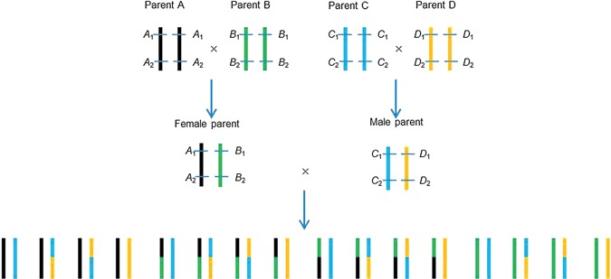
Diagram of the development of a double cross population from four inbred lines A, B, C, and D, which are homozygous at most loci Assuming locus 1 and locus 2 were two linked polymorphism markers. A1, B1, C1, and D1 were the four alleles at marker locus 1. A2, B2, C2, and D2 were the four alleles at marker locus 2. Linkage phases in the two single crosses were known when the four inbred lines were genotyped.
Quantitative trait locus (QTL) mapping is a critical step in gene fine mapping, map‐based cloning, and the efficient use of gene information in molecular breeding. In the past 20 to 30 years, QTL mapping in bi‐parental populations has been well developed and widely used (Lander and Botstein 1989; Zeng 1994; Li et al. 2007, 2008; Yi et al. 2007; Zhang et al. 2008; Wang 2009). Inclusive composite interval mapping (ICIM) has been developed and applied in additive, dominance and epistatic mapping in bi‐parental populations (Li et al. 2007, 2008; Zhang et al. 2008; Wang 2009). A two‐step mapping strategy was used in ICIM. Firstly, stepwise regression was conducted to select the significant marker variables in additive and dominance mapping or marker pairs in epistatic mapping. Then the phenotypic values were adjusted by the significant variables except the two (or more in epistatic mapping) flanking the current scanning positions, so as to completely control the QTL effects outside the scanning intervals (i.e. background control). The precise background control in ICIM results in sharp and clear peaks around the QTL locations, which can be an advantage in separating linked QTL (Li et al. 2012). Some QTL mapping methods consider QTL effects directly in the statistical models (Xu 1996; Ao and Xu 2006). ICIM first gives maximum likelihood estimates of QTL genotypic values, from which the genetic effects can be calculated directly. Genotypic values have direct applications in breeding, as the favorable genotypes can be easily identified.
Compared with bi‐parental populations, QTL mapping methods are less investigated in genetic populations of clonal F1 and double cross. Groover et al. (1994) used analysis of variance (ANOVA) to detect QTL affecting wood specific gravity in an outbred pedigree of loblolly pine. Xu (1996) proposed a multiple linear regression analysis for QTL detection in double cross. To improve the efficiency of method in Xu (1996); Ao and Xu (2006) used the expectation‐maximization (EM) algorithm in maximum likelihood estimation. The modified method improved detection power, but the estimated effects of QTL were biased with large standard errors. Interval mapping and multiple‐QTL models (MQM) were implemented in software MAPQTL for QTL mapping in clonal F1 (van Ooijen 2009). Composite interval mapping (CIM; Zeng 1994) and MQM were implemented in package R/qtl (Broman et al. 2003) for QTL mapping in phase‐known double crosses.
In double crosses, alleles at each polymorphic locus can be traced back to the four inbred lines, when the four lines have been genotyped. Genotypes of the two single crosses are known (Figure 1). In clonal F1, linkage phases in both parents can be determined by linkage analysis, from which four haploids can be built. If the four haploids could be viewed as haploids of the four inbred lines in a double cross, clonal F1 is equivalent to double cross (Zhang et al. 2015). Therefore, we only consider double cross populations for QTL mapping in this study. Our objectives in this study were: (1) to identify and classify all informative markers based on the number of distinguishable alleles and the number of distinguishable genotypes; (2) to impute incomplete and missing markers using the completed linkage maps; (3) to develop an inclusive linear model capable of absorbing all genetic effects; (4) to extend the ICIM algorithm for QTL detection in clonal F1 and double cross populations; (5) to validate the proposed methods in simulated populations and one actual maize double cross population.
RESULTS
QTL analysis for genetic model I
Likelihood of odd (LOD) profile, phenotypic variation explained (PVE), additive and dominance effects from ICIM in a simulated population with a size of 500 were shown in Figure 2. One peak can be clearly seen in the middle of the chromosome (49 cM, close to the true position of 50 cM) with a LOD score of 52.96 (Figure 2A). The estimated genotypic values of four QTL genotypes at the peak were 24.49, 10.76, 10.26 and 0.96, close to the respective true values 25, 10, 10 and 0. The identified QTL explained 49.29% of the phenotypic variation, close to the true broad sense heritability of 0.5 (Figure 2B). Female and male additive effects of the identified QTL were estimated at 6.01, and 5.76 (Figure 2C), respectively, which were close to the true value 6.25. Estimate of dominance effect at the peak was 1.11 (Figure 2D), close to the true value 1.25.
Figure 2.
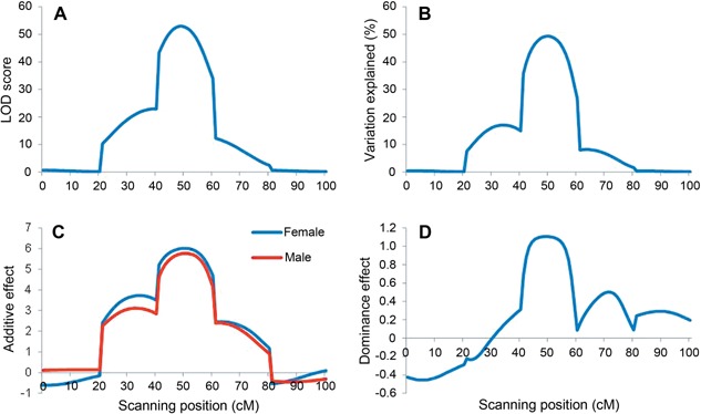
Mapping results for a simulated double cross population with a size of 500 by inclusive composite interval mapping (ICIM) in genetic model I (A, B, C), and (D) are profiles of Likelihood of odd (LOD) score, phenotypic variation explained (PVE), female and male additive effects, and dominance effect, respectively.
There are five marker intervals on the simulated chromosome, each of 20 cM in length. QTL was located in the third interval. ICIM achieved close‐to‐zero LOD scores at chromosomal regions far away from the true QTL position, and high LOD scores at the QTL interval and the two neighboring intervals. A sharp peak was observed at the true QTL position (Figure 2A). In the test statistic profile of Figure 1 in Xu (1996) a peak was also observed at the true QTL position, but the test statistic was not close to zero at chromosomal regions far away from the true QTL. In comparison, peak of LOD scores from ICIM was much clearer and sharper than the peak observed in Xu (1996).
The close‐to‐zero LOD scores at the first and last marker intervals were the results of background control in ICIM. For the simulated genetic model, variables involving markers 3 and 4 should be included in the inclusive linear model (see Material and Methods for details), and other variables have a coefficient of zero. When scanning at the first interval, for example, genetic variation from the QTL located on the third interval was completely controlled by the seven variables of markers 3 and 4. Therefore, only random error effects affect the LOD score. At the second interval, genetic variation from the QTL located on the third interval was only partially controlled by the effects of marker 4, leaving part of the QTL variation, which was quantified by the effects of marker 3. Therefore, both random error effects and the remaining QTL variation affect the LOD score. At the third interval, whole genetic variation from the QTL was retained, as markers 3 and 4 were not used in adjusting the phenotype. Both random error effects and the whole QTL variation affect the LOD score. QTL located at the third marker interval may affect the multiple tests along the whole chromosome.
Power analysis of ICIM for genetic models II and III
Inclusive composite interval mapping was applied in 1,000 simulated double cross populations for genetic models II and III. Detection powers increased with the increase in PVE of QTL and population size for both genetic models (Figure 3). For example, PVE of QTL 1 to 3 were 5%, 10% and 15% in genetic model II. Their detection powers were 30.4%, 65.3%, 86.1% for population size 200 (Figure 3A), and 85.1%, 98.4% and 99.9% for population size 500 (Figure 3B), respectively. The increase in population size not only improved the detection power of ICIM, but also reduced its FDR. FDR was 16.41% for population size 200 and 7.94% for population size 500 in model II (Figure 3A, B); and FDR was 15.75% for population size 200 and 6.62% for population size 500 in model III (Figure 3C, D).
Figure 3.
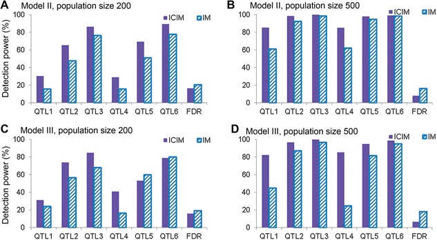
Power analysis from 1,000 simulated populations by inclusive composite interval mapping (ICIM) and IM in genetic models II and III (A) Model II, and population size 200, (B) model II, and population size 500, (C) model III, and population size 200, (D) model III, and population size 500. The support interval for each predefined quantitative trait locus (QTL) was set at 20 cM, and the Likelihood of odd (LOD) threshold was 3.75. The last bar represents the false discovery rate (FDR).
When powers were calculated for all marker intervals along the eight chromosomes, the probability that QTL were mapped onto the two devoid chromosomes (i.e., chromosomes 7 and 8) was rather low (Figure 4). Most QTL identified were around the predefined QTL for both genetic models (Figure 4). In other words, false positives were around the true QTL positions and were less likely to be located in chromosomal regions far from the predefined QTL or in chromosomes where no QTL were located. For example, QTL1 was located at 25 cM on chromosome 1 in genetic model II. When population size was 500, power at the marker interval where QTL1 was located was 63.3%, and powers at its left and right intervals were 13.0%, and 15.5%, respectively. Powers at other intervals on chromosome 1 were close to 0.
Figure 4.
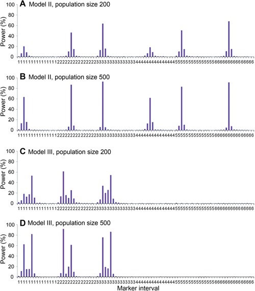
Power analysis of every marker interval on chromosomes 1 to 6 from 1,000 simulated populations by inclusive composite interval mapping (ICIM) in genetic models II and III There was no quantitative trait locus (QTL) predefined on chromosomes 7 and 8 in both genetic models, and the powers of intervals on chromosomes 7 and 8 were close to zero. (A) Model II, and population size 200, (B) model II, and population size 500, (C) model III, and population size 200, (D) model III, and population size 500. Power was calculated as the proportion of runs that detected the presence of QTL for each interval.
In genetic model III, linked QTL became easier to be separated when the population size was larger, especially for QTL with small PVE (Figure 4C, D). For instance, QTL1 and QTL2 were linked on chromosome 1. When population size was 200, powers at the marker intervals where QTL1 and QTL2 were located were 18.4%, and 53.0%, respectively. Powers at the left and right marker intervals of QTL1 were 6.0%, and 12.7%, respectively. Powers at the left and right marker intervals of QTL2 were 17.5%, and 11.0%, respectively. When population size was 500, powers at the marker intervals where QTL1 and QTL2 were located were 62.2%, and 81.7%, respectively. Powers at the left and right marker intervals of QTL1 were 10.9%, and 14.6%, respectively. Powers at the left and right marker intervals of QTL2 were 14.8%, and 6.4%, respectively. Obviously, detection power was increased at the QTL interval, but was reduced at its left and right intervals as the increase of population size.
Estimation of QTL locations and effects for genetic models II and III by ICIM
Estimated QTL locations and effects from 1,000 simulated populations by ICIM were shown in Table 1 for genetic model II and Table S1 for genetic model III. Unbiased estimates of QTL locations and effects were observed under both genetic models and population sizes. Taking population size 200 and QTL1 as an example, its estimated position, aF, aM and d were 24.82, 1.95, 0.58 and –0.02 in genetic model II, and 25.79, 1.78, 0.93 and 0.28 in genetic model III, corresponding to the true values 25, 1.5, 0.5 and 0, respectively. The standard errors of these estimates were 4.73, 0.43, 0.52, and 0.58 in model II, and 5.11, 0.55, 0.96 and 0.54 in model III, respectively (Tables 1, S1).
Table 1.
Estimated quantitative trait locus (QTL) locations and genetic effects from 1,000 simulations by inclusive composite interval mapping (ICIM) in genetic model II
| Population size | Estimate | QTL1 | QTL2 | QTL3 | QTL4 | QTL5 | QTL6 |
|---|---|---|---|---|---|---|---|
| 200 | LOD score | 5.47 | 6.69 | 8.32 | 5.43 | 6.66 | 8.40 |
| (1.64)a | (2.02) | (2.61) | (1.46) | (2.11) | (2.77) | ||
| Position (cM) | 24.82 | 54.96 | 24.91 | 54.60 | 24.87 | 54.89 | |
| (4.73) | (4.54) | (4.30) | (5.07) | (4.38) | (4.15) | ||
| aF | 1.94 | 0.03 | –0.43 | –2.00 | 0.00 | –0.46 | |
| (0.43) | (0.47) | (0.46) | (0.35) | (0.48) | (0.46) | ||
| aM | 0.58 | 2.17 | 2.52 | –0.51 | –2.16 | –2.53 | |
| (0.52) | (0.47) | (0.50) | (0.54) | (0.46) | (0.53) | ||
| d | –0.02 | 0.96 | 0.89 | 0.05 | –0.98 | –0.89 | |
| (0.58) | (0.52) | (0.52) | (0.52) | (0.52) | (0.52) | ||
| 500 | LOD score | 7.93 | 13.22 | 19.25 | 7.95 | 13.21 | 19.21 |
| (2.66) | (3.59) | (4.21) | (2.52) | (3.65) | (4.12) | ||
| Position (cM) | 24.85 | 54.95 | 24.91 | 54.75 | 25.00 | 55.16 | |
| (4.36) | (3.29) | (2.72) | (4.41) | (3.53) | (2.73) | ||
| aF | 1.54 | 0.00 | –0.45 | –1.55 | 0.00 | –0.43 | |
| (0.29) | (0.28) | (0.30) | (0.28) | (0.27) | (0.28) | ||
| aM | 0.48 | 1.97 | 2.46 | –0.46 | –1.97 | –2.46 | |
| (0.31) | (0.33) | (0.31) | (0.29) | (0.35) | (0.32) | ||
| d | 0.00 | 0.89 | 0.90 | –0.01 | –0.89 | –0.91 | |
| (0.33) | (0.37) | (0.38) | (0.31) | (0.37) | (0.38) |
The number in parentheses is the standard error.
The deviation between the estimate and true value decreased with the increase in population size, as well as the standard error of the estimate for both genetic models. In genetic model II for population size 500, position, aF, aM and d of QTL1 were averagely estimated at 24.85, 1.54, 0.48 and 0.00, the corresponding deviations to their true values were –0.15, 0.04, –0.02, and 0.00, and their standard errors were 4.36, 0.29, 0.31, and 0.33 (Table 1). In comparison, deviations of position, aF, aM and d of QTL1 were –0.18, 0.45, 0.08 and –0.02, and standard errors were 4.73, 0.43, 0.52, and 0.58 for population size 200, respectively (Table 1). In genetic model III and for population size 500, position, aF, aM and d of QTL1 were averagely estimated at 24.75, 1.54, 0.42 and 0.12, the corresponding deviations to their true values were –0.25, 0.04, –0.08, and 0.12, and their standard errors were 4.25, 0.29, 0.39, and 0.32 (Table S1). In comparison, deviations of position, aF, aM and d of QTL1 were 0.79, 0.28, 0.43 and 0.28, and standard errors were 5.11, 0.55, 0.96 and 0.54 for population size 200, respectively (Table S1).
Comparison of ICIM with IM
Detection powers of ICIM and IM from 1,000 simulations with population sizes 200 and 500 for genetic models II and III were shown in Figure 3. In genetic model II and for population size 200, powers of IM were 15.7%, 47.6%, 76.3%, 15.7%, 51.1% and 77.7% for QTL1 through QTL6, and FDR was 20.5%; powers of ICIM were 30.4%, 65.3%, 86.1%, 29.0%, 69.2%, and 89.2%, and FDR was 16.41% (Figure 3A), respectively. The increase in population size improved the detection powers of both IM and ICIM for all predefined QTL, and also reduced the FDR. But, IM still had lower detection power and higher FDR (Figure 3B). The similar trend was observed in genetic model III (Figure 3C, D).
Estimated QTL locations and effects from 1,000 simulated populations for IM were shown in Tables S2 and S3. Similar to ICIM, unbiased estimates of QTL locations were observed under both population sizes and genetic models. However, some estimates of QTL effects were biased in IM, and the deviations between the estimates and true values of QTL positions and effects were larger by IM than ICIM, especially for linked QTL and QTL with smaller PVE. Taking population size 200 and QTL1 as an example, deviations of estimated position, aF, aM and d by IM were 0.29, 0.73, 0.29 and –0.15 in model II (Table S2), which were higher than those by ICIM, i.e. –0.18, 0.45, 0.08 and –0.02, respectively (Table 1). Deviations of estimated position, aF, aM and d by IM were 1.54, 0.34, 1.60 and –0.05 in model III (Table S3), which were higher than those by ICIM, i.e. 0.79, 0.28, 0.43 and 0.28, respectively (Table S1). Estimated aF of QTL1 by IM was biased in genetic model II and estimated aM of QTL1 by IM was biased in genetic model III.
Comparison of ICIM with MQM and CIM
The first five simulated populations with a size of 200 in genetic model II were used for comparison of ICIM with MQM and CIM. The estimated locations and effects of detected QTL were shown in Table S4 (Supplementary Materials). As there was no estimated effect at each position from R/qtl for double crosses, QTL effects by CIM were the corresponding values at the closest markers. ICIM detected 5, 5, 4, 6 and 4 QTL in the five simulated populations, respectively. When a support interval of 20 cM centered at the true QTL location was used, 21 of the detected QTL were true, and the other three were false. QTL1 to 6 were detected in 3, 4, 4, 1, 4 and 5 of the five populations, respectively. MQM detected 4, 6, 6, 5 and 4 QTL in the five populations, respectively, among which 18 were true, and seven were false. QTL1 to 6 were detected in 1, 3, 5, 1, 3 and 5 of the five populations, respectively. CIM detected 3, 4, 3, 5 and 4 QTL in the five populations, respectively, among which 16 were true, and three were false. QTL1 to 6 were detected in 1, 3, 3, 1, 3 and 5 of the five populations, respectively. Detection powers of MQM and CIM were lower than ICIM, and FDR of MQM and CIM were much higher than ICIM.
For most QTL in the support intervals (i.e. true QTL), their estimated positions and effects were close to their true values in both methods, although some deviation was observed. For example, QTL3 was detected by ICIM, MQM and CIM in the first simulated population. The estimated position, aF, aM and d by ICIM were 25, –0.56, 3.33 and 0.94; estimates by MQM were 26, –0.42, 3.29 and 1.13, estimates by CIM were 24, –0.13, 2.53 and 0.74, corresponding to the true values 25, –0.5, 2.5 and 1 (Table S4).
ICIM in a simulated population with five categories of markers
To further illustrate the outcomes of ICIM, we conducted QTL mapping on the first double cross population in genetic model II with 500 individuals. The genotypic values of the four inbred lines were 24, 34, 34 and 0, respectively, and the genotypic values of the female and male parents were 29 and 33. Phenotypic values in double cross progenies showed continuous distribution similar to typical quantitative traits. There is no clear classification of the phenotype, and it is impossible to deduce the number of QTL without the assistance of molecular markers.
By QTL mapping, six clear peaks on the first six chromosomes could be seen along the one‐dimensional LOD profile, indicating six unlinked QTL (Figure 5A). The chromosomes or chromosomal regions not harboring QTL had LOD scores close to 0. The estimated positions of the six QTL were 23, 52, 28, 57, 29 and 50 cM close to the true QTL positions 25, 55, 25, 55, 25 and 55 cM on the first six chromosomes, respectively (Table 2). The estimated aF were 1.82, 0.03, –0.21, –2.32, –0.37, and –0.06 (Table 2, Figure 5B); the estimated aM were 0.86, 1.82, 2.77, –0.41, –1.82, and –2.38 (Table 2, Figure 5C); the estimated d were 1.07, 0.63, 0.95, 0.07, –1.00 and –1.11, respectively (Table 2, Figure 5D). The estimated effects at peak positions were close to the true values given in Table 3, although some discrepancies were observed.
Figure 5.
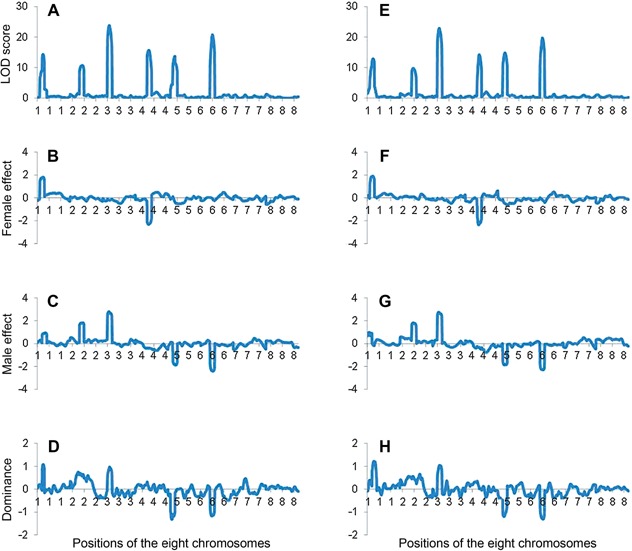
Mapping results for the first simulated double cross population with a size of 500 by inclusive composite interval mapping (ICIM) in genetic model II (A, B, C), and (D) are profiles of Likelihood of odd (LOD) score, female additive effect, male additive effect, and dominance effect, respectively, when there is no missing marker information. (E, F, G), and (H) are profiles of LOD score, female additive effect, male additive effect, and dominance effect, respectively, when two thirds of markers have missing information.
Table 2.
Estimated quantitative trait locus (QTL) locations and effects from the first simulated double cross population with population size 500 by inclusive composite interval mapping (ICIM) in genetic model II
| QTL | Chromosome | Position (cM) | LOD score | Genetic effects | PVE (%)a | Genotypic mean | |||||
|---|---|---|---|---|---|---|---|---|---|---|---|
| aF | aM | d | AqCq | AqDq | BqCq | BqDq | |||||
| No missing and incomplete markers | |||||||||||
| QTL1 | 1 | 23 | 14.34 | 1.82 | 0.86 | 1.07 | 8.31 | 32.88 | 29.02 | 27.1 | 27.53 |
| QTL2 | 2 | 52 | 10.72 | 0.03 | 1.82 | 0.63 | 5.69 | 31.61 | 26.71 | 30.29 | 27.91 |
| QTL3 | 3 | 28 | 23.83 | –0.21 | 2.77 | 0.95 | 13.6 | 32.67 | 25.24 | 31.18 | 27.54 |
| QTL4 | 4 | 57 | 15.64 | –2.32 | –0.41 | 0.07 | 8.58 | 26.43 | 27.09 | 30.92 | 31.88 |
| QTL5 | 5 | 29 | 13.67 | –0.37 | –1.82 | –1.00 | 7.47 | 25.94 | 31.57 | 28.67 | 30.31 |
| QTL6 | 6 | 50 | 20.78 | –0.06 | –2.38 | –1.11 | 11.07 | 25.57 | 32.55 | 27.92 | 30.45 |
| 2/3 markers are incomplete | |||||||||||
| QTL1 | 1 | 24 | 12.87 | 1.89 | –0.12 | 1.11 | 7.63 | 32.12 | 30.13 | 26.13 | 28.58 |
| QTL2 | 2 | 56 | 9.79 | 0.10 | 1.81 | 0.56 | 5.50 | 31.65 | 26.9 | 30.32 | 27.81 |
| QTL3 | 3 | 28 | 22.86 | –0.09 | 2.72 | 1.03 | 13.44 | 32.81 | 25.32 | 30.95 | 27.56 |
| QTL4 | 4 | 59 | 14.22 | –2.29 | –0.32 | 0.06 | 8.27 | 26.57 | 27.08 | 31.02 | 31.78 |
| QTL5 | 5 | 30 | 14.81 | –0.48 | –1.81 | –1.08 | 7.87 | 25.79 | 31.56 | 28.91 | 30.37 |
| QTL6 | 6 | 50 | 19.70 | –0.17 | –2.27 | –1.28 | 10.78 | 25.42 | 32.51 | 28.31 | 30.28 |
Phenotypic variation explained by the identified QTL.
Table 3.
Estimated quantitative trait locus (QTL) locations and genetic effects affecting day to silking in the actual double cross maize population
| QTL | Chromosome | Position (cM) | LOD score | Genetic effects | PVE (%)a | Genotypic mean | |||||
|---|---|---|---|---|---|---|---|---|---|---|---|
| aF | aM | d | AqCq | AqDq | BqCq | BqDq | |||||
| qDS2 | 2 | 201 | 12.23 | 0.23 | –0.61 | 0.43 | 16.02 | 72.08 | 72.43 | 70.76 | 72.83 |
| qDS4 | 4 | 75 | 5.87 | 0.21 | –0.44 | 0.12 | 6.26 | 71.89 | 72.54 | 71.24 | 72.37 |
| qDS7 | 7 | 142 | 6.16 | 0.60 | –0.09 | 0.01 | 9.54 | 72.54 | 72.70 | 71.33 | 71.53 |
| qDS9 | 9 | 79 | 7.98 | 0.53 | –0.20 | –0.05 | 8.16 | 72.30 | 72.81 | 71.34 | 71.64 |
Phenotypic variation explained by the identified QTL.
For results given in Figure 5A–D, all markers belonged to Category I. To illustrate the performance of ICIM for different marker categories, two‐thirds of markers (i.e. 80 markers) in this population were randomly assigned to other four categories. In other words, 20 markers each were Categories II to V, and 40 markers were Category I. When the five categories were present, the six predefined QTL could still be detected (Figure 5E). The estimated positions of the six QTL were 24, 56, 28, 59, 30 and 50 cM close to the true QTL positions (Table 2). Profiles of genetic effect estimates were similar to those in the original population (Figure 5F, G, H). For the six predefined QTL, the estimated aF were 1.89, 0.10, –0.09, –2.29, –0.48 and –0.17; the estimated aM were –0.12, 1.81, 2.72, –0.32, –1.81, and –2.27; the estimated d were 1.11, 0.56, 1.03, 0.06, –1.08 and –1.28, respectively (Table 2). The estimates of QTL positions and effects were still close to their true values.
QTL on days to silking in maize detected by ICIM
Days to silking of the four inbred lines were 80.86, 75.00, 69.20 and 88.33 d, respectively (Li et al. 2013). The distribution of days to silking in the double cross population was shown in Figure 6A. Among the 219 markers in the linkage map, 81, 61, 51, 15 and 11 markers were Categories I to V respectively. A total of 3,913 marker points were missing, representing 6.45% of total marker points. Segregation distortions were observed for a few markers as well. There was no missing phenotypic data. LOD scores, and estimated additive and dominance effects (i.e. a F, a M and d) along the maize genome were shown in Figures 6B–D.
Figure 6.
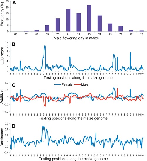
Mapping results of days to silking by inclusive composite interval mapping (ICIM) in the actual maize double cross population with a size of 277 progenies (A) Phenotypic distribution, (B) Likelihood of odd (LOD) score, (C) additive effect of the female and male parents, (D) dominance effect between the female and male parents. The scanning step was 1 cM
Under LOD threshold 3.96, four QTL were identified on days to silking: one each on chromosomes 2, 4, 7 and 9 (Table 3). The detected QTL explained a total of 39.49% of phenotypic variation. qDS2 was located at 201 cM on chromosome 2, explaining the largest PVE of 16.02%. Its LOD score was 12.23, and estimated genetic effects were 0.23, –0.61 and 0.43. The estimated genotypic values of AqCq, AqDq, BqCq and BqDq were 72.08, 72.43, 70.76 and 72.83, respectively. qDS4 was located at 75 cM on chromosome 4 with the smallest PVE of 6.26%. Its LOD score was 5.87, and the estimated genetic effects were 0.21, –0.44 and 0.12. Estimated genotypic values of AqCq, AqDq, BqCq and BqDq were 71.89, 72.54, 71.24 and 72.37, respectively.
DISCUSSION
Equivalence of clonal F1 and double cross
Double crosses are made between four inbred lines. Alleles A, B, C and D at each polymorphic locus in the progenies can be traced back to their four inbred parents, when the four lines have been genotyped. Therefore, genotype of the single cross between lines A and B is A 1 B 1/A 2 B 2; and genotype of the single cross between lines C and D is C 1 D 1/C 2 D 2 (Figure 1). Linkage phases are known in double crosses.
In clonal F1 progenies, genotype of the female parent can be either A 1 B 1/A 2 B 2 or A 1 B 2/B 1 A 2; and genotype of the male parent can be either C 1 D 1/D 2 D 2 or C 1 D 2/D 1 C 2. The unknown linkage phases in clonal F1 will complicate the procedure of QTL analysis. Fortunately, linkage phases in both parents of the clonal F1 can be determined by linkage analysis, from which four haploids can be built. If the four haploids could be viewed as haploids of the four inbred lines in a double cross, clonal F1 is equivalent to double cross (Zhang et al. 2015).
Marker categories in double cross
In double cross populations, each marker locus is classified into five categories based on the number of identifiable alleles in parents and the number of identifiable genotypes in F1 progenies (Figure 7). The two classification factors need to be considered at the same time. For marker categories I, IV and V, there are two identifiable alleles in both parents, but the number of identifiable genotypes in F1 progenies is four for Category I, and three for Categories IV and V. The reason is that for marker category IV and V, the female and male parents have the same genotype. For Categories II and III, the number of identifiable genotypes in F1 progenies is for both categories. The method to distinguish the two categories is to identify the number of alleles in parents. For Category II, alleles A and B are equal; there are two identifiable alleles in the male parent, but only one identifiable allele in the female parent. For Category III, alleles C and D are equal; there are two identifiable alleles in the female parent, but only one identifiable allele in the male parent.
Figure 7.
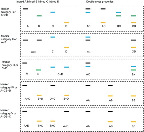
Five categories of polymorphism markers which can be used for genetic studies in double cross populations In Category I or ABCD, each marker shows four identifiable alleles between the four inbred parents, represented by A, B, C and D (see the four different colors in Figure 1). In the double cross population, four genotypes can be identified, represented by AC, AD, BC and BD. In Category II or A = B, one allele can be seen in parents A and B, and two alleles can be seen in parents C and D. Only two genotypes can be identified, represented by XC and XD, where X can be either A or B. In Category III or C = D, two alleles can be seen in parents A and B, and one allele can be seen in parents C and D. The two identifiable genotypes are represented by AX and BX, where X can be either C or D. In Category IV or A = CB = D, parents A and C show the same homozygous genotype, and parents B and D show the same homozygous genotype. In Category V or A = DB = C, parents A and D show the same homozygous genotype, and parents B and C show the same homozygous genotype. In both categories, the two alleles in four parents are represented by A and B, and three genotypes in their progenies are represented by AA, AB and BB.
For Category I, one allele in the female parent may be the same as one allele in the male parent. For example, allele A may be equal to C. The number of identifiable alleles in parents is three, but there are still four identifiable genotypes in F1 progenies. For Category II, the allele in the female parent can be the same as one allele in the male parent. For example, alleles A, B and C are equal. There is no polymorphism in the female parent, but there are still two identifiable genotypes in F1 progenies. For Category III, the allele in the male parent can be the same as one allele in the female parent. For example, alleles A, C and D are equal. There is no polymorphism in the male parent, but there are still two identifiable genotypes in F1 progenies.
Extension of ICIM to genetic populations of clonal F1 and double cross
Inclusive composite interval mapping was firstly proposed for QTL mapping in biparental populations (Li et al. 2007; Zhang et al. 2008; Wang 2009). Informative markers in double cross progenies can be classified into five categories (Figure 7). Only Category I (or ABCD) represents the case of fully informative markers. Other category markers provide incomplete information, due to the confounding of genotypes. Using the completed linkage maps, incomplete and missing markers can be imputed to Category I markers, so that QTL mapping can be developed on fully informative markers. In the most simple single‐locus QTL model, it was shown that dominance between the female and male parents can cause the interactions between markers. In order to completely absorb all QTL effects, the linear model of phenotype on marker genotype should include marker variables and marker interactions. In clonal F1 and double cross, the interval mapping on phenotypes adjusted by the estimated linear model retains all advantages of ICIM in biparental populations over other mapping methods, such as higher detection power, lower FDR, and less biased estimation of QTL positions and effects (Li et al. 2007, 2010b, 2012; Zhang et al. 2008; Wang 2009).
Further consideration on genetic analysis of double cross
In addition to additive and dominance, epistasis is another important source of variation of complex traits. ICIM has been extended for mapping epistatic QTL in biparental populations (Li et al. 2008; Zhang et al. 2012). It has been shown that ICIM is able to identify epistatic QTL no matter whether the two interacting QTL have any additive effects. In ICIM epistatic QTL mapping, unbiased estimates of QTL locations and effects can be achieved. Detection power is largely affected by population size, heritability of epistasis, and the amount and distribution of genetic effects (Zhang et al. 2012). We are currently considering the ICIM epistatic QTL mapping for clonal F1 and double cross.
In self‐ and cross‐pollinated species, genetic populations consisting of homozygous lines are preferred, such as doubled haploids (DHs) and recombinant inbred lines (RILs). In such populations, phenotypic traits can be investigated in multi‐environment replicated trials, allowing more precise phenotypic evaluation and the study of genotype by environment interactions. In practice, DH or RIL could also be developed from a double cross. We understand that this may not be the case for clonal species, but is applicable for both self‐ and cross‐pollinated species. We are considering the extension of ICIM in DH or RIL population of a double cross as well.
MATERIALS AND METHODS
Marker categories and coding criteria
Five marker categories can be differentiated on the number of identifiable alleles in the four original lines and the number of identifiable genotypes in their double cross progenies (Figure 7). Category I (or ABCD) represents the case of fully informative markers. Each marker shows four identifiable alleles in the four inbred parents, represented by A, B, C and D (see the four different colors in Figure 1). In the double cross progenies, four genotypes can be identified, represented by AC, AD, BC and BD, respectively (Figure 7). When no distortion occurs, the four genotypes will follow the Mendelian ratio of 1:1:1:1. It needs to be mentioned that it is not necessary that all four alleles are distinct. It is possible that one female allele is the same as one male allele. For example, allele A is equal to allele C.
Category II (or A = B) represents the case of male‐polymorphism markers. Only one allele can be seen in parents A and B, but two alleles can be seen in parents C and D. Genotypes AC and BC cannot be separated, and neither can genotypes AD and BD. In this category, XC is used to code genotypes AC and BC; and XD is used to code genotypes AD and BD, where X stands for either allele A or allele B (Figure 7). When no distortion occurs, the two genotypes will follow the Mendelian ratio of 1:1. Category III (or C = D) represents the case of female‐polymorphism markers. Two alleles can be seen in parents A and B, but only one allele can be seen in parents C and D. Genotypes AC and AD cannot be separated, neither can genotypes BC and BD. In this category, AX is used to code genotypes AC and AD; and BX is used to code genotypes BC and BD, where X stands for either allele C or D (Figure 7). When no distortion occurs, the two genotypes will follow the Mendelian ratio of 1:1.
Category IV (or A = CB = D) and Category V (or A = DB = C) represent the case of co‐dominant markers. By co‐dominant markers, we mean they show the same polymorphism pattern in both female and male parents, similar to the F2 populations derived from two inbred parents in self‐ and cross‐pollinated species. In Category IV, parents A and C show the same homozygous genotype; parents B and D show the same homozygous genotype. In Category V, parents A and D show the same homozygous genotype, and parents B and C show the same homozygous genotype. The two alleles in four parents are represented by A and B, and three genotypes in their progenies are represented by AA, AB and BB (Figure 7). When no distortion occurs, the three genotypes will follow the Mendelian ratio of 1:2:1.
For any category, missing values of marker type are coded as XX.
Imputation of incomplete and missing marker information
Among the five categories (Figure 7), only Category I markers are fully informative for genetic analysis, i.e. there are four identifiable genotypes at the marker locus. Markers of Categories II to V provide partial information, i.e. some of the four genotypes are confounded. The completed linkage maps can be used for imputing incomplete markers and missing markers types. For markers belonging to Category II, genotype XC will be replaced by either AC or BC, and genotype XD will be replaced by either AD or BD. For markers belonging to Category III, genotype AX will be replaced by either AC or AD, and genotype BX will be replaced by either BC or BD. For markers belonging to Category IV, genotype AA will be replaced by AC, genotype AB will be replaced by either AD or BC and genotype BB will be replaced by BD. For markers belonging to Category V, genotype AA will be replaced by AD, genotype AB will be replaced by either AC or BD and genotype BB will be replaced by BC. For complete missing marker types XX, it will be replaced by either AC, AD, BC or BD. After imputation, all markers will belong to Category I, which has four informative genotypes AC, AD, BC and BD. This imputation will greatly simplify the linkage mapping approaches of quantitative trait genes. The imputation algorithm of incomplete and missing marker information is followed.
(1) No linkage information available
For any incomplete or missing marker type in one individual, if there is no non‐missing Category I marker linked, the incomplete and missing marker type will be imputed by the Mendelian ratio at the marker locus. For example, if one locus is Category II and has marker type XC in one progeny, XC can be either AC or BC with equal chance. Therefore, the incomplete genotype XC is imputed to AC or BC by the ratio of 1:1, as given in Equation 1. If the marker is completely missing in one progeny, missing genotype XX is imputed to AC, AD, BC or BD by the ratio of 1:1:1:1, as given in Equation 2.
| (1) |
| (2) |
(2) One linked fully‐informative marker
If there is one non‐missing Category I marker linked, the incomplete and missing marker type will be imputed by the conditional probabilities on the fully informative genotypes. Conditional probabilities are calculated from observed frequencies of the 16 marker classes (see the first three columns in Table 4). Assume genotype at locus 1 is A 1 C 1, and locus 2 is Category II and has genotype X 2 C 2. The ratio of two conditional probabilities that locus 2 has genotype A 2 C 2 or B 2 C 2 was . The incomplete genotype X 2 C 2 is imputed to either A 2 C 2 or B 2 C 2 by the ratio of two conditional probabilities, given in Equation 3. If marker type at locus 2 is completely missing in one progeny, missing genotype X 2 X 2 is imputed to either A 2 C 2, A 2 D 2, B 2 C 2 or B 2 D 2 by the ratio of four conditional probabilities, given in Equation 4.
| (3) |
| (4) |
where is the estimate of recombination frequency between the two marker loci.
Table 4.
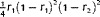
Frequency of quantitative trait locus (QTL) genotype under each marker class in a double cross population. r1, r2 and r were combined recombination frequencies between the left marker and QTL, QTL and the right marker, two markers on the combined linkage map
| Left marker | Right marker | Frequency | QTL genotype | ||||||||
|---|---|---|---|---|---|---|---|---|---|---|---|
| AqCq | AqDq | BqCq | BqDq | ||||||||
| A 1 C 1 | A 2 C 2 |
|
|
|
|
|
|||||
| A 1 C 1 | A 2 D 2 |
|
|
|
|
|
|||||
| A 1 D 1 | A 2 C 2 |
|
|
|
|
|
|||||
| A 1 D 1 | A 2 D 2 |
|
|
|
|
|
|||||
| A 1 C 1 | B 2 C 2 |
|
|
|
|
|
|||||
| A 1 C 1 | B 2 D 2 |
|
|
|
|
|
|||||
| A 1 D 1 | B 2 C 2 |
|
|
|
|
|
|||||
| A 1 D 1 | B 2 D 2 |
|
|
|
|
|
|||||
| B 1 C 1 | A 2 C 2 |
|
|
|
|
|
|||||
| B 1 C 1 | A 2 D 2 |
|
|
|
|
|
|||||
| B 1 D 1 | A 2 C 2 |
|
|
|
|
|
|||||
| B 1 D 1 | A 2 D 2 |
|
|
|
|
|
|||||
| B 1 C 1 | B 2 C 2 |
|
|
|
|
|
|||||
| B 1 C 1 | B 2 D 2 |
|
|
|
|
|
|||||
| B 1 D 1 | B 2 C 2 |
|
|
|
|
|
|||||
| B 1 D 1 | B 2 D 2 |
|
|
|
|
|
|||||
(3) Two linked fully‐informative flanking markers
If there are two non‐missing Category I markers linked on both sides, the incomplete and missing marker type will be imputed by conditional probabilities on the fully informative genotypes at the two flanking markers. Conditional probabilities are calculated from the observed frequencies of the 64 genotypes in Table 4. Assume genotypes of the two flanking markers are A 1 C 1 and A 2 C 2, and marker q is Category II having genotype XqCq. The incomplete genotype XqCq can be imputed to either AqCq or BqCq with the ratio of two conditional probabilities, given in Equation 5. If marker q is completely missing in one progeny, missing genotype XqXq is imputed to either AqCq, AqDq, BqCq or BqDq by the ratio of four conditional probabilities, given in Equation 6.
| (5) |
| (6) |
where and are the estimates of recombination frequencies between the left marker and the missing locus, and between the missing locus and the right marker, respectively.
One‐locus model in the double cross progenies
Assume Aq, Bq, Cq and Dq are the four alleles at one QTL in a double cross population. Genotypic value of an individual with known QTL genotype, i.e. AqCq, AqDq, BqCq or BqDq, is written in the one‐locus additive and dominance model, i.e. Equation 7.
| (7) |
where is mean of the four QTL genotypes, aF and aM are the additive genetic effects of the female and male parents, d is the dominance effect between the female and male parents, and u and v are the independent indicators of QTL genotypes valued at 1 and 1 for AqCq, 1 and –1 for AqDq, –1 and 1 for BqCq, and –1 and –1 for BqDq. From Equation 7, genotypic mean, and the three defined genetic effects can be calculated, as shown in Equation 8.
| (8) |
where are mean performances (or genotypic values) of the four QTL genotypes AqCq, AqDq, BqCq and BqDq. When there is no segregation distortion, genetic variation contributed by the QTL is given in Equation 9.
| (9) |
Assuming A 1, B 1, C 1, D 1 and A 2, B 2, C 2, D 2 are the four alleles at two markers flanking the QTL, there are a total of 16 identifiable marker classes in the double cross population (Table 4). Two indicators (represented by x and y, respectively) occur for each marker locus, similarly defined as indicators u and v of QTL genotype in Equation 7. Based on the expected frequency of QTL genotype in each marker class (Table 4), mean of each marker class can be calculated as well (Table 5). Similarly to QTL effects, we can define the additive effects of the left marker, i.e. F 1, and M 1, additive effects of the right marker, i.e. F 2, and M 2, dominance effects, i.e. FM 11 for the left marker, and FM 22 for the right marker, and additive by additive marker interactions between the female and male parents, i.e. FM 12 and FM 21. Other types of marker effects can also be defined, but can be proved to be 0, under the additive and dominance QTL model (see Supplementary Materials for proof).
Table 5.
Expectations of the quantitative trait locus (QTL) indicators, and mean performance for each marker class. r 1, r 2 and r were combined recombination frequencies between the left marker and QTL, QTL and the right marker, two markers on the combined linkage map
| Left marker | Right marker | x 1 | y 1 | x 2 | y 2 |
|
|
|
Marker class mean | ||||
|---|---|---|---|---|---|---|---|---|---|---|---|---|---|
| A 1 C 1 | A 2 C 2 | 1 | 1 | 1 | 1 |
|
|
|
|
||||
| A 1 C 1 | A 2 D 2 | 1 | 1 | 1 | –1 |
|
|
|
|
||||
| A 1 D 1 | A 2 C 2 | 1 | –1 | 1 | 1 |
|
|
|
|
||||
| A 1 D 1 | A 2 D 2 | 1 | –1 | 1 | –1 |
|
|
|
|
||||
| A 1 C 1 | B 2 C 2 | 1 | 1 | –1 | 1 |
|
|
|
|
||||
| A 1 C 1 | B 2 D 2 | 1 | 1 | –1 | –1 |
|
|
|
|
||||
| A 1 D 1 | B 2 C 2 | 1 | –1 | –1 | 1 |
|
|
|
|
||||
| A 1 D 1 | B 2 D 2 | 1 | –1 | –1 | –1 |
|
|
|
|
||||
| B 1 C 1 | A 2 C 2 | –1 | 1 | 1 | 1 |
|
|
|
|
||||
| B 1 C 1 | A 2 D 2 | –1 | 1 | 1 | –1 |
|
|
|
|
||||
| B 1 D 1 | A 2 C 2 | –1 | –1 | 1 | 1 |
|
|
|
|
||||
| B 1 D 1 | A 2 D 2 | –1 | –1 | 1 | –1 |
|
|
|
|
||||
| B 1 C 1 | B 2 C 2 | –1 | 1 | –1 | 1 |
|
|
|
|
||||
| B 1 C 1 | B 2 D 2 | –1 | 1 | –1 | –1 |
|
|
|
|
||||
| B 1 D 1 | B 2 C 2 | –1 | –1 | –1 | 1 |
|
|
|
|
||||
| B 1 D 1 | B 2 D 2 | –1 | –1 | –1 | –1 |
|
|
|
|
Equation S2 indicates that the QTL additive effect aF only causes marker additive effects of the female parent (i.e. F 1 and F 2), and the QTL additive effect aM only causes marker additive effects of the male parent (i.e. M 1 and M 2). But the QTL dominance effect d causes the additive by additive marker interactions between the female and male parents (i.e., FM 12 and FM 21), as well as the dominance effects between the female and male parents at the same marker (i.e., FM 11 and FM 22). The non‐zero marker interactions FM 12, and FM 21, caused by the QTL dominance effect, indicate that marker variables by themselves cannot completely absorb the effects of QTL located between the two markers. This phenomenon has been observed in the F2 populations as well (Zhang et al. 2008). In general, we can define the genotypic value of an individual with known marker types as in Equation 10.
| (10) |
where x 1 and y 1 are the indicators for the left marker valued at 1 and 1 for marker type A 1 C 1, 1 and –1 for A 1 D 1, –1 and 1 for B 1 C 1, and –1 and –1 for B 1 D 1, x 2 and y 2 are the indicators for the right marker valued at 1 and 1 for marker type A 2 C 2, 1 and –1 for A 2 D 2, –1 and 1 for B 2 C 2, and –1 and –1 for B 2 D 2.
The expectation of u, v and uv under each marker class can be proved as in Equation 11.
| (11) |
where , , and f 1 and f 2 are defined in Table 5. So the genotypic value of a double cross individual with known marker class can be represented by marker variables and four marker multiplications as in Equation (12).
| (12) |
The inclusive linear model of phenotype on marker type
For simplicity, we assume there are m QTL located on m intervals defined by m+1 markers on one chromosome. The genotypic value of a double cross individual is defined as in Equation 13.
, j=1, 2, …, m for each QTL;
| (13) |
where uj and vj are the indicators for genotypes at the j th QTL. By using Equations 11 and 12, the genotypic value of a double cross progeny with known marker types can be re‐organized as in Equation 14.
| (14) |
where
,
,
where
,
,
where
, and , where
The inclusive linear model containing all markers simultaneously is shown in Equation 15, which explains the three genetic effects of each QTL.
| (15) |
where P is the phenotypic value of the trait of interest, and is the random environmental error. It can be seen that coefficients in Equation 15 are only affected by the neighboring QTL. In other words, the QTL effects will be completely absorbed by the seven variables of the two closest markers (regarding as one variable). Therefore, if estimated carefully, all QTL effects would be included in the linear model of Equation 15, based on which the background genetic variation could be well controlled in QTL interval mapping.
Inclusive composite interval mapping (ICIM) of QTL
Assume there are n progenies in a double cross population. Similar to QTL mapping in bi‐parental populations, two steps are included in ICIM (Li et al. 2007; Zhang et al. 2008). In the first step, we consider using stepwise regression to estimate the parameters in Equation 15. Coefficients of those variables not retained by stepwise regression were set at 0. In the second step, traditional interval mapping (Lander and Botstein 1989) is conducted on the adjusted phenotypic values, i.e.,
| (16) |
where k and k+1 represent the two flanking markers of the current scanning interval, representing the n progenies in the double cross population, and the hat symbol means “estimated”. The adjusted values in Equation 16 contain all the location and effect information of QTL in the current interval, but at the same time, QTL in other chromosomal intervals have been completely controlled (Li et al. 2007; Zhang et al. 2008). At a testing position in the interval [k, k+1], phenotypes of the four QTL genotypes AqCq, AqDq, BqCq and BqDq are assumed to be normally distributed as , where k=1, 2, 3, 4 represent the four QTL genotypes, respectively. The two hypotheses used to test the existence of a QTL at the scanning position are:
vs
: at least two of , , and are not equal.
The logarithm likelihood under HA is, therefore,
| (17) |
where represents the progenies belonging to the marker class (j=1, 2, …, 16), (k=1, 2, 3, 4) is the conditional probability of the QTL genotype in the marker class (Table 4), and is the density function of the normal distribution . EM algorithm to calculate the maximum likelihood estimates in Eq. (17) and LOD score can be found in Supplementary Materials.
Empirical formula of the LOD threshold in QTL mapping
LOD threshold is used to control false positive in QTL mapping and determines the number of identified QTL. Sun et al. (2013) indicated that the number of independent tests (denoted as Meff) depends on the genome length, marker density and population type in one‐dimensional scanning of additive QTL in single–environment analysis. For example for the genome‐wide type I error rate of =0.05, a marker density of 10 cM and a backcross population, Meff was about 0.072 times the genome length. Given the number of independent tests, empirical LOD threshold using the Bonferroni correction can be calculated as in Equation 18.
| (18) |
where is the type‐I error per scanning test, df is the degree of freedom equal to difference between the numbers of independent genetic parameters to be estimated under the null hypothesis and the alternative hypothesis, and is the inverse χ 2 distribution that returns the critical value of a right‐tailed probability αp for the degree of freedom df.
In clonal F1 and double cross populations, there were four genotypes at each locus. Under the alternative hypothesis, each QTL genotype has its own distribution, and the number of independent genetic parameters to be estimated is 4. Under the null hypothesis, the four QTL genotypes have the same distribution, and there is only one genetic parameter to be estimated. So df is 3 in QTL mapping of double cross populations. So a suitable LOD threshold can also be determined by Equation 18 given the genome‐wide type I error, total genome size and the average marker density of the linkage map.
Three QTL distribution models in simulation
In this study, we simulated three QTL distribution models to illustrate the efficiency of ICIM in clonal F1 and double cross, i.e. genetic models I, II and III. In these models, we predefined different genomic information, such as number of chromosomes, number and positions of markers, QTL positions and effects and so on. In genetic model I, we considered a simple model consisting of only one chromosome with a length of 100 cM, as used in Xu (1996). Six full‐informative markers were evenly distributed on the chromosome and one QTL was located in the middle of the chromosome. Values of the four QTL genotypes AqCq, AqDq, BqCq and BqDq were 25, 10, 10 and 0, respectively, from which the three genetic effects aF, aM and d were calculated as 6.25, 6.25 and 1.25, respectively. The broad sense heritability was set at 0.5.
In genetic model II, we considered six QTL with different effects and a genome consisting of eight chromosomes (Table 6). Each chromosome was of 140 cM in length, with 15 evenly distributed co‐dominant markers. QTL1 had additive effect aF = 1.5 and aM = 0.5, without dominance. QTL2 had additive effect aM = 2 and dominance effect = 1, without female additive effect aF. QTL3 had additive effect aF =–0.5 and aM = 2.5, and dominance effect d = 1. QTL4 had additive effect aF =–1.5 and aM =–0.5, without dominance. QTL5 had additive effect aM =–2 and dominance effect =–1, without female additive effect aF. QTL6 had additive effect aF =–0.5 and aM =–2.5, and dominance effect d =–1. These QTL were distributed on different chromosomes. No interactions between QTL were considered. Each QTL was assumed to be located in the middle of a marker interval (Table 6). QTL3 and QTL6 each explained 25% of the genotypic variation and 15% of the phenotypic variance under broad sense heritability 0.6. QTL2 and QTL5 each explained 16.67% of the genotypic variation and 10% of the phenotypic variance.QTL1 and QTL4 each explained 8.33% of the genotypic variation and 5% of the phenotypic variance which were the least among the six predefined QTL (Table 6).
Table 6.
Six putative quantitative trait locus (QTL) and their distributions for genetic model II in a genome consisting of eight chromosomes, each of 140 cM and evenly distributed by 15 markers. Heritability in the broad sense was set at 0.6 for a trait in interest
| QTL | Additive effect aF | Additive effect aM | Dominance effect d | Position (model II) | Variation explained (%) | ||
|---|---|---|---|---|---|---|---|
| Chrom. | cM | Genotypic | Phenotypic | ||||
| QTL1 | 1.5 | 0.5 | 0 | 1 | 25 | 8.33 | 5.00 |
| QTL2 | 0 | 2 | 1 | 2 | 55 | 16.67 | 10.00 |
| QTL3 | –0.5 | 2.5 | 1 | 3 | 25 | 25.00 | 15.00 |
| QTL4 | –1.5 | –0.5 | 0 | 4 | 55 | 8.33 | 5.00 |
| QTL5 | 0 | –2 | –1 | 5 | 25 | 16.67 | 10.00 |
| QTL6 | –0.5 | –2.5 | –1 | 6 | 55 | 25.00 | 15.00 |
In genetic model III, we also considered six QTL, whose genetic effects were the same as defined in model II. However, QTL1 and QTL2 were linked on chromosome 1 at positions 25 and 55 cM; QTL 3 and QTL4 were linked on chromosome 2 at positions 25 and 55 cM; QTL 5 and QTL6 were linked on chromosome 3 at positions 25 and 55 cM. No interactions between QTL were considered.
Double cross populations were simulated by the genetics and breeding simulation tool of QuLine (Wang et al. 2003, 2004). All markers in the simulated populations had four different alleles. QTL mapping of methods IM and ICIM was conducted in the software GACD (available from www.isbreeding.net). QTL mapping by method MQM was conducted in the software MAPQTL 6.0 (van Ooijen 2009). QTL mapping by method CIM was conducted in the package R/qtl (Broman et al. 2003). One population with a size of 500 was simulated for genetic model I, same as Xu (1996). A total of 1,000 populations with sizes 200 and 500 were simulated for genetic models II and III, respectively. The two probabilities for entering and removing variables for the ICIM stepwise regression were set at 0.001 and 0.002. The method for selecting cofactors in MQM was backward selection with P‐value 0.02. The beginning cofactors were markers at every 20 cM on all map groups. The threshold LOD score used was set at 2.63 for ICIM in genetic model I, and 3.75 for all mapping methods in models II and III, which were derived from the empirical formula under = 0.05. The scanning step was set at 1 cM. Other mapping factors for CIM were set as default in R/qtl.
Each simulated QTL was assigned to a support interval of 20 cM centered at the true QTL location, and the power was estimated by the support interval. QTL identified in other intervals were viewed as false positives. In the support interval, if multiple peaks occurred, only the highest one was counted. In other chromosome regions, all peaks higher than the LOD threshold were counted, regardless of the distance between the significant peaks. More details on power and false discovery rate (FDR) calculation can be found in Li et al. (2010b, 2012) and Zhang et al. (2012).
To illustrate the performance of ICIM for different marker categories, a new population was generated from the first simulated double cross population of 500 individuals in genetic model II. Two‐thirds of markers (i.e. 80 markers) in this population were randomly assigned to either of Categories II, III, IV, or V.
One double cross population in maize
The actual double cross population used in this study was derived from four maize inbred lines, developed by College of Agronomy, Henan Agricultural University (Li et al. 2013). The population consists of 277 double cross individuals. Two single crosses were firstly made in Zhengzhou, Henan, China, in summer 2008. One was between maize inbred lines 276 and 72, and the other was between maize inbred lines A188 and Jiao51. The two single crosses were then planted in Ledong, Hainan, China, in winter 2008, and the double cross was made at the flowering stage. The double cross population was planted in Zhengzhou in spring 2009 for phenotyping. Polymorphism of SSR molecular markers was firstly screened in the two single crosses. Then the double cross population was genotyped by 220 polymorphism SSR markers. The original four parental lines were not genotyped. Therefore linkage phases in this population are unknown, and the linkage analysis method of clonal F1 is applicable.
Days to silking was investigated in the field in 2009. The genetic linkage map was constructed by 219 SSR molecular markers using the software GACD. One marker was unlinked with others, and was deleted before QTL analysis. The whole genome was of 1778.09 cM with 10 chromosomes, and the average marker distance was 8.51 cM. Each chromosome had 16 to 28 relatively evenly distributed markers. ICIM was used for QTL mapping, and parameters for analysis were set the same as the genetic models, except that LOD threshold was set at 3.96, which was derived from the empirical formula under
DATA ARCHIVING
GACD, integrated genetic analysis software for clonal F1 and double cross populations, can be accessed from http://www.isbreeding.net
Supporting information
Additional supporting information may be found in the online version of this article at the publisher's web‐site.
Equation S1. Relationship between marker class mean and marker effects
Equation S2. Relationship between marker effects and QTL effects
Table S1. Estimated QTL locations and genetic effects from 1,000 simulations by ICIM in genetic model III
Table S2. Estimated QTL locations and effects from 1,000 simulations by IM in genetic model II
Table S3. Estimated QTL locations and genetic effects from 1,000 simulations by IM in genetic model III
Table S4. Detected QTL in the first five simulated double cross population with population size 200 by ICIM, MQM and CIM in genetic model II
ACKNOWLEDGEMENTS
This work was supported by the National Hi‐Tech Research and Development Program of China (2012AA101104‐1), the National Natural Science Foundation of China (project no. 31200917), the Generation and HarvestPlus Challenge Program of CGIAR, and the Agricultural Science and Technology Innovation Program of Chinese Academy of Agricultural Sciences (CAAS).
Zhang L, Li H, Ding J, Wu J, Wang J ( 2015) Quantitative trait locus mapping with background control in genetic populations of clonal F1 and double cross. J Integr Plant Biol 57: 1046–1062
Available online on Apr. 22, 2015 at www.wileyonlinelibrary.com/journal/jipb
REFERENCES
- Allard RW ( 1999) Principles of Plant Breeding. 2nd eds John Wiley BT & Sons, Inc. New York, NY: [Google Scholar]
- Ao Y, Xu C ( 2006) Maximum likelihood method for mapping QTL in four‐way cross design. Acta Agron Sin 32: 51–56 (in Chinese with an English abstract) [Google Scholar]
- Broman KW, Wu H, Sen Ś, Churchill GA ( 2003) R/qtl: QTL mapping in experimental crosses. Bioinformatics 19: 889–890 [DOI] [PubMed] [Google Scholar]
- Carlier JD, Reis A, Duval MF, D's Eeckenbrugge GC, Leitão JM ( 2004) Genetic maps of RAPD, AFLP and ISSR markers in Ananas bracteatus and A. comosus using the pseudo‐testcross strategy. Plant Breed 123: 186–192 [Google Scholar]
- Collins A, Milbourne D, Ramsay L, Meyer R, Chatot‐Balandras C, Oberhagemann P, De Jong W, Gebhardt C, Bonnel E, Waugh R ( 1999) QTL for field resistance to late blight in potato are strongly correlated with maturity and vigour. Mol Breed 5: 387–398 [Google Scholar]
- Fregene M, Angel F, Gomez R, Rodriguez F, Chavarriaga P, Roca W, Tohme J, Bonierbale M ( 1997) A molecular genetic map of cassava (Manihot esculenta Crantz). Theor Appl Genet 95: 431–441 [Google Scholar]
- Groover A, Devey M, Fiddler T, Lee J, Megraw R, Mitchel‐Olds T, Sherman B, Vujcic S, Williams C, Neale D ( 1994) Identification of quantitative trait loci influencing wood specific gravity in an outbred pedigree of loblolly pine. Genetics 138: 1293–1300 [DOI] [PMC free article] [PubMed] [Google Scholar]
- Hemmat M, Weeden NF, Manganaris AG, Lawson DM ( 1994) Molecular marker linkage map for apple. J Hered 85: 4–11 [PubMed] [Google Scholar]
- Kunkeaw S, Tangphatsornruang S, Smith DR, Triwitayakorn K ( 2010) Genetic linkage map of cassava (Manihot esculenta Crantz) based on AFLP and SSR markers. Plant Breed 129: 112–115 [Google Scholar]
- Lander ES, Botstein D ( 1989) Mapping Mendelian factors underlying quantitative traits using RFLP linkage maps. Genetics 121: 185–199 [DOI] [PMC free article] [PubMed] [Google Scholar]
- Li A, Liu Q, Wang Q, Zhang L, Zhai H, Liu S ( 2010a) Establishment of molecular linkage maps using SRAP markers in sweet potato. Acta Agron Sin 36: 1286–1295 (in Chinese with an English abstract) [Google Scholar]
- Li H, Ye G, Wang J ( 2007) A modified algorithm for the improvement of composite interval mapping. Genetics 175: 361–374 [DOI] [PMC free article] [PubMed] [Google Scholar]
- Li H, Ribaut JM, Li Z, Wang J ( 2008) Inclusive composite interval mapping (ICIM) for digenic epistasis of quantitative traits in biparental populations. Theor Appl Genet 116: 243–260 [DOI] [PubMed] [Google Scholar]
- Li H, Hearne S, Bänziger M, Li Z, Wang J ( 2010b) Statistical properties of QTL linkage mapping in biparental genetic populations. Heredity 105: 257–267 [DOI] [PubMed] [Google Scholar]
- Li H, Zhang L, Wang J ( 2012) Estimation of statistical power and false discovery rate of QTL mapping methods through computer simulation. Chin Sci Bull 57: 2701–2710 [Google Scholar]
- Li Y, Li X, Chen J, Zhou B, Zhou Z, Ding J, Wu J ( 2013) Identification of QTL for traits related to flowing time in maize based on four‐way cross population. J Henan Agric Univ 47: 231–240 (in Chinese with an English abstract) [Google Scholar]
- Liu X, Mao J, Lu X, Ma L, Aitken KS, Jackson PA, Cai Q, Fan Y ( 2010) Construction of molecular genetic linkage map of sugarcane based on SSR and AFLP markers. Acta Agron Sin 36: 177–183 (in Chinese with an English abstract) [Google Scholar]
- Sun Z, Li H, Zhang L, Wang J ( 2013) Properties of the test statistic under null hypothesis and the calculation of LOD threshold in quantitative trait loci (QTL) mapping. Acta Agron Sin 39: 1–11 (in Chinese with an English abstract) [Google Scholar]
- Tanksley SD, Ganal MW, Prince JP, de Vicente MC, Bonierbale MW, Broun P, Fulton TM, Giovannoni JJ, Grandillo S, Martin GB, Messeguer R, Miller JC, Miller L, Paterson AH, Pineda O, Röder MS, Wing RA, Wu W, Young ND ( 1992) High density molecular linkage maps of the tomato and potato genomes. Genetics 132: 1141–1160 [DOI] [PMC free article] [PubMed] [Google Scholar]
- van Ooijen JW ( 2009) MapQTL 6, software for the mapping of quantitative trait loci in experimental populations of diploid species. Kyazma BV, Wageningen, Netherlands
- van Os H, Andrzejewski S, Bakker E, Barrena I, Bryan GJ, Caromel B, Ghareeb B, Isidore E, de Jong W, van Koert P, Lefebvre V, Milbourne D, Ritter E, van der Voort JNAMR, Rousselle‐Bourgeois F, van Vliet J, Waugh R, Visser RGF, Bakker J, van Eck HJ ( 2006) Construction of a 10,000‐marker ultradense genetic recombination map of potato: Providing a framework for accelerated gene isolation and a genomewide physical map. Genetics 173: 1075–1087 [DOI] [PMC free article] [PubMed] [Google Scholar]
- Wang J ( 2009) Inclusive composite interval mapping of quantitative trait genes. Acta Agron Sin 35: 239–245 (in Chinese with an English abstract) [Google Scholar]
- Wang J, van Ginkel M, Podlich D, Ye G, Trethowan R, Pfeiffer W, DeLacy IH, Cooper M, Rajaram S ( 2003) Comparison of two breeding strategies by computer simulation. Crop Sci 43: 1764–1773 [Google Scholar]
- Wang J, van Ginkel M, Trethowan R, Ye G, Delacy I, Podlich D, Cooper M ( 2004) Simulating the effects of dominance and epistasis on selection response in the CIMMYT Wheat Breeding Program using QuCim. Crop Sci 44: 2006–2018 [Google Scholar]
- Xu S ( 1996) Mapping quantitative trait loci using four‐way crosses. Genet Res 68: 175–181 [Google Scholar]
- Yamamoto T, Kimura T, Shoda M, Imai T, Saito T, Sawamura Y, Kotobuki K, Hayashi T, Matsuta N ( 2002) Genetic linkage maps constructed by using interspecific Cross between Japanese and European pears. Theor Appl Genet 106: 9–18 [DOI] [PubMed] [Google Scholar]
- Yi, N , Banerjee S, Pomp D, Yandell BS ( 2007) Bayesian mapping of genomewide interacting quantitative trait loci for ordinal traits. Genetics 176: 1855–1864 [DOI] [PMC free article] [PubMed] [Google Scholar]
- Zeng Z ( 1994) Precision mapping of quantitative trait loci. Genetics 136: 1457–1468 [DOI] [PMC free article] [PubMed] [Google Scholar]
- Zhang L, Li H, Li Z, Wang J ( 2008) Interactions between markers can be caused by the dominance effect of quantitative trait loci. Genetics 180: 1177–1190 [DOI] [PMC free article] [PubMed] [Google Scholar]
- Zhang L, Li H, Wang J ( 2012) The statistical power of Inclusive composite interval mapping int detecting digenic epistasis showing common F2 segregation ratios. J Integr Plant Biol 54: 270–279 [DOI] [PubMed] [Google Scholar]
- Zhang L, Li H, Wang J ( 2015) Linkage analysis and map construction in genetic populations of clonal F1 and double cross. G3‐Genes Genom Genet 5: 427–439 [DOI] [PMC free article] [PubMed] [Google Scholar]
- Zhang X, Yin T, Zhuge Q, Huang M, Zhu L, Zhai W, W R, Wang M ( 2000) RAPD linkage mapping in a Populus deltoids × Populus euramericana F1 family. Hereditas (Beijing) 22: 209–213 (in Chinese with an English abstract) [Google Scholar]
Associated Data
This section collects any data citations, data availability statements, or supplementary materials included in this article.
Supplementary Materials
Additional supporting information may be found in the online version of this article at the publisher's web‐site.
Equation S1. Relationship between marker class mean and marker effects
Equation S2. Relationship between marker effects and QTL effects
Table S1. Estimated QTL locations and genetic effects from 1,000 simulations by ICIM in genetic model III
Table S2. Estimated QTL locations and effects from 1,000 simulations by IM in genetic model II
Table S3. Estimated QTL locations and genetic effects from 1,000 simulations by IM in genetic model III
Table S4. Detected QTL in the first five simulated double cross population with population size 200 by ICIM, MQM and CIM in genetic model II