Abstract
Purpose:
Current approaches using deformable vector field (DVF) for motion-compensated 4D-cone beam CT (CBCT) reconstruction typically utilize an isotropically smoothed DVF between different respiration phases. Such isotropically smoothed DVF does not work well if sliding motion exists between neighboring organs. This study investigated an anisotropic motion modeling scheme by extracting organ boundary local motions (e.g., sliding) and incorporated them into 4D-CBCT reconstruction to optimize the motion modeling and reconstruction methods.
Methods:
Initially, a modified simultaneous algebraic reconstruction technique (mSART) was applied to reconstruct high quality reference phase CBCT using all phase projections. The initial DVFs were precalculated and subsequently updated to achieve the optimized solution. During the DVF update, sliding motion estimation was performed by matching the measured projections to the forward projection of the deformed reference phase CBCT. In this process, each moving organ boundary was first segmented. The normal vectors of the boundary DVF were then extracted and incorporated for further DVF optimization. The regularization term in the objective function adaptively regularizes the DVF by (1) isotopically smoothing the DVF within each organ; (2) smoothing the DVF at boundary along the normal direction; and (3) leaving the tangent direction of boundary DVF unsmoothed (i.e., allowing for sliding motion). A nonlinear conjugate gradient optimizer was used. The algorithm was validated on a digital cubic tube phantom with sliding motion, nonuniform rotational B-spline based cardiac-torso (NCAT) phantom, and two anonymized patient data. The relative reconstruction error (RE), the motion trajectory’s root mean square error (RMSE) together with its maximum error (MaxE), and the Dice coefficient of the lung boundary were calculated to evaluate the algorithm performance.
Results:
For the cubic tube and NCAT phantom tests, the REs are 10.2% and 7.4% with sliding motion compensation, compared to 13.4% and 8.9% without sliding modeling. The motion trajectory’s RMSE and MaxE for NCAT phantom tests are 0.5 and 0.8 mm with sliding motion constraint compared to 3.5 and 7.3 mm without sliding motion modeling. The Dice coefficients for both NCAT phantom and the patients show a consistent trend that sliding motion constraint achieves better similarity for segmented lung boundary compared with the ground truth or patient reference.
Conclusions:
A sliding motion-compensated 4D-CBCT reconstruction and the motion modeling scheme was developed. Both phantom and patient study demonstrated the improved accuracy and motion modeling accuracy in reconstructed 4D-CBCT.
Keywords: sliding motion, 4D-CBCT, deformable vector field, organ motion
1. INTRODUCTION
Verification of a moving target just before the treatment beam delivery is a challenging task. The concept of 4D cone-beam CT (4D-CBCT) offers a powerful tool to achieve this goal. However, its clinical application is limited. One reason is related to the limited number of projections within each respiration phase. Under 1 min gantry scanning protocol, around 670 projections were acquired for reconstructing 10-phase 4D-CBCT.1,2 The projection number available at each sorted phase is not sufficient for FDK to achieve a good reconstruction, which leads to severe streaking artifacts on the reconstructed image.
Recently, various 4D-CBCT reconstruction methods have been proposed.1–15 One major category from these methods is deformable vector field (DVF) based 4D-CBCT reconstruction,2,4,5,7,8,14 and it has shown a good capability to obtain high quality 4D-CBCT. One method from this category is called simultaneous motion estimation and image reconstruction (SMEIR),14 in which the 4D-DVFs are simultaneously updated along with the motion-compensated reconstruction by a modified simultaneous algebraic reconstruction technique (mSART). The DVFs are directly obtained by matching the measured CBCT projection and the forward projection of high quality reference phase CBCT with motion compensation. Both phantom and patient studies had demonstrated the ability of SMEIR on improving the 4D-CBCT reconstruction quality as well as the lung motion tracking accuracy. However, the original SMEIR method does not consider the sliding motion between the lung and thoracic cage. The optimization energy function is designed based on an isotropic smoothing penalty term for the DVF updating. However, organs can have anisotropic motion, especially at the organ surface contacting sites such as the lung-to-thoracic interface or lung-to-heart interface. A uniform smoothing term design ignores the organ local nonuniform motion such as sliding motion at the organ boundary sites. The final estimated DVF solution may not always achieve an optimized solution if the sliding motion at the organ boundary sites is not properly modeled.
Sliding motion has been previously modeled to improve the deformable registration accuracy in 4D-CT imaging.16–19 In this work, we take the sliding motion into consideration for accurate 4D-CBCT reconstruction. Specifically, the DVF smoothing term is redesigned and is divided into two parts: (1) the inner organ smoothing part; and (2) the organ boundary sliding modeling part. The isotropic DVF smoothing will be performed at the organ inner sites, and the adaptive anisotropic DVF smoothing will be performed at the organ boundary sites to capture the sliding motion in the DVF. The sliding motion at the organ boundary has also be considered in a multiorgan meshing model20 in which motion fields were defined on sparse mesh grids. In this work, the motion fields are defined on each voxel with a dense representation. A simple sliding digital cubic tube phantom is used to initially test the effectiveness of this new regularization design. A nonuniform rotational B-spline based cardiac-torso (NCAT) phantom is used to further validate the algorithm. Two patient data are also tested to demonstrate the effectiveness of our algorithm.
2. METHODS AND MATERIALS
2.A. Overview of SMEIR algorithm
As mentioned in Ref. 14, the mSART reconstruction is first applied by using all sorted 4D projections to achieve a high quality reference motion-compensated phase (e.g., 0% phase). Then the DVF estimation is performed for each phase by matching the measured CBCT projection of the target phase to the forward projection of the deformed motion-compensated reference phase. Mathematically, let denote the log-transformed 4D-CBCT projection (i.e., line integral) from phase t, and denote the attenuation coefficients of the phase t image, the mSART is given by
| (1) |
| (2) |
where k is the iteration step, j is the voxel index of phase 0% while n is the voxel index of phase t; ain is the intersection length of projection ray i with voxel n, which is obtained by a ray-tracing technique;21 and denotes the element of the inverse DVF that deforms phase t to phase 0. The initial image is first reconstructed by the total variation (TV) minimization22 reconstruction to achieve a noise suppressed initial reference phase image (0% phase). Equation (2) describes the forward deformation that deforms phase 0 4D-CBCT to phase t. For projection matching, an inverse consistent DVF estimation is applied by designing a symmetric energy function,
| (3) |
where f1 and f2 denote the symmetric energy function; 0 stands for phase 0%, t stands for any other phase t; A is the projection matrix; v0→t denotes the forward DVF; and vt→0 denotes the inverse DVF. and are the data fidelity terms of the inverse consistent cost function. and are the corresponding regularization terms. The inverse consistent constraint is shown in the last term of Eq. (3). β controls the trade-off between the data fidelity term and smoothing regularization term . In the original SMEIR method, we assume the smoothness of DVF is isotropic everywhere, and is designed by
| (4) |
where ∂vi/∂xj denotes the difference between neighboring voxels for each DVF component along three directions. A nonlinear conjugate gradient optimizer was used for estimating the final DVF solution.
2.B. Sliding motion regularization design
As mentioned before, one limitation of the SMEIR smoothing term is that the DVF smoothing is always isotropic everywhere. However, sliding motion frequently happens at the organ boundary sites. If we relied on isotropic DVF smoothing everywhere, the local sliding motion will be ignored in the final reconstruction results. To take the sliding motion along organ boundaries into account, we redesigned the regularization term in the DVF smoothing for those voxels located at the organ boundary. The new anisotropic penalty term Ref. 23 was redesigned as
| (5) |
where I is the identity matrix, is the normal vector to the lung organ boundary voxel x; vl is the lth scalar component of DVF and is the lth scalar component of the normal directions to the organ surface DVF. Let be the lth normal scalar component, then . As the normal directions to the organ surface are different for different voxels, the sliding motion considered in this work is in 3D. Each original organ boundary voxel is extended ±1 voxel to its neighborhood along the x, y, z directions, so the thickness of the boundary is 3 × 3 × 3 voxels. Then each organ boundary voxels is assigned with different weightings. The weighting term is defined by , with λ being empirically set at 0.2 mm−1 for all simulated phantom data and patient data in our study. With λ = 0.2 mm−1, we can achieve clear and naturally smoothed boundary. Too large or too small lambda values will make the boundary either blurred or bumpy with disconnected points. is the distance to the central voxel within each 3 × 3 × 3 boundary thickness range. is 1 at the boundary central layer and decreases with increased distance . As the objective function is minimized by the nonlinear conjugate gradient optimization, the gradient of is calculated by
| (6) |
where div denotes the divergence operator, el is the lth canonical unit vector (e.g., ex = [1, 0, 0]T).
The segmentation of lung was performed by the itk-snap software.24 A rectangular region of interest (ROI) box was first defined manually to just include the lung region. Once the ROI was defined, the lung region was extracted by carefully tuning the intensity threshold. The boundary of lung was identified by the active contour model and the segmented lung was saved as mesh surface data. The surface voxel normal vectors for each voxel were then extracted by MeshLab software (meshlab.sourceforge.net) directly. The gradient and divergence operation were calculated within the 3 × 3 × 3 neighborhood surrounding each voxel of interest.
2.C. DVF initial for optimization
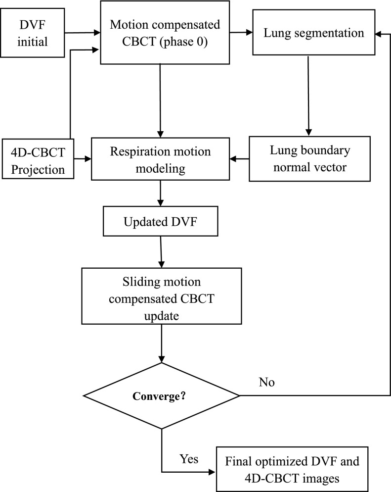
The simultaneous sliding motion-compensated 4D-CBCT reconstruction workflow chart is illustrated in Fig. 1. 10-phase 4D-CBCT is first reconstructed by TV minimization from corresponding projections after phase sorting. Then demons registration25 is used to obtain the DVF initials to start the motion-compensated reconstruction and inverse consistent DVF optimization. The code used for demons registration algorithm was downloaded from Ref. 26, where the implementation was based on Ref. 27. If predefined DVFs are not available (i.e., using zero DVFs in the first SART reconstruction), an initially reconstructed reference CBCT will be blurred. The following motion estimation step will fail as we are comparing the forward projections of the reference CBCT to measured projections of other phases during the DVF estimation.
FIG. 1.
Flow chart of the sliding motion-compensated 4D-CBCT reconstruction.
2.D. Evaluation criteria
2.D.1. Reconstruction accuracy
The relative error (RE) between the reconstructed 4D-CBCT with sliding constraint and the ground truth or reference was used to quantify the image reconstruction accuracy by defining
| (7) |
where is the phantom ground truth, is the reconstructed image.
2.D.2. Tumor motion accuracy
The tumor motion trajectory was extracted from the reconstructed images and the ground truth. The root mean square error (RMSE) and maximum error (MaxE) of the estimated tumor position were analyzed to quantify motion estimation accuracy with sliding motion constraint.
| (8) |
where denotes the estimated image feature point position for the ph-th phase and denotes the corresponding position from the ground truth. MaxE is defined as the maximum error of the tumor position extracted from all 9 phases.
2.D.3. Dice coefficient
We used the Dice coefficient to measure the segmented lung boundary contours to see whether sliding motion-compensated result has more contour similarity compared with the truth reference. Let A be the contour area obtained from the result with or without sliding motion compensation, and B is the contour from the truth reference. The Dice coefficient s given by
| (9) |
In our study, we use the voxel number within the organ contour as a surrogate of the exact area.
3. RESULTS
3.A. Sliding cubic tube phantom
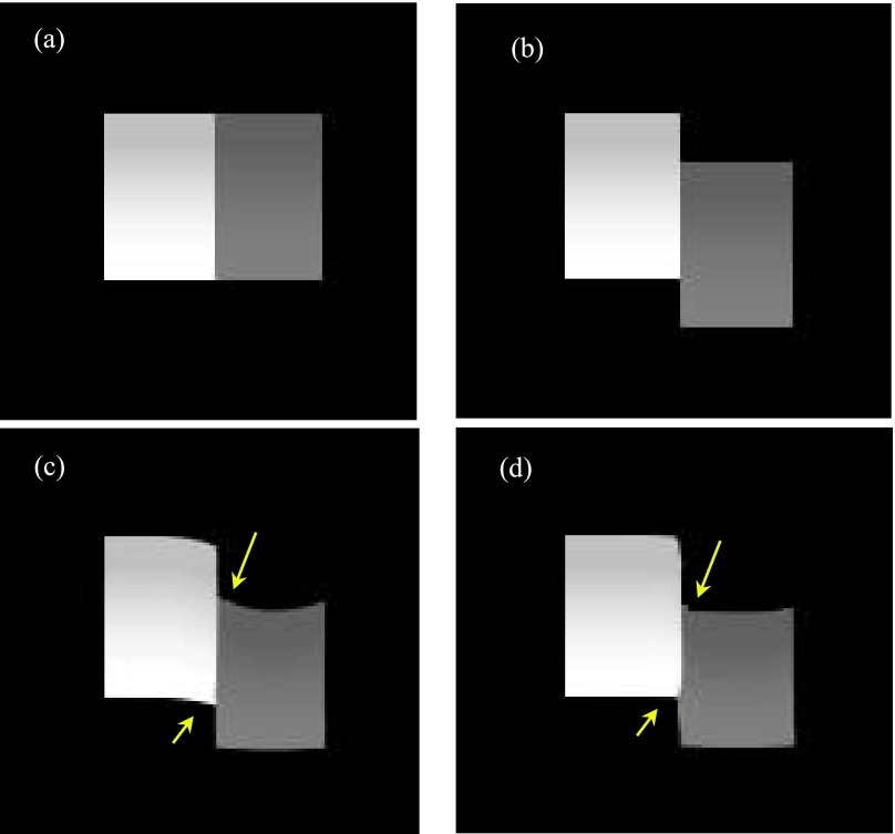
A simple digital sliding tube phantom (Fig. 2) was simulated to validate the algorithm effectiveness. The sliding tube phantom was designed with one cubic tube static while the other one slides against the static one along 90° and 45°. The tube intensity changed gradually within the range of 0.015–0.019 mm−1 for the gray tube and 0.031–0.044 mm−1 for the white tube. The forward projections of the phantom were generated with 20 views per phase for both of the initial and target phases according to CBCT geometry. The sliding motion for the moving tube is 15 mm. The simulated voxel size is 2 mm, and the detector element size is 2 mm. The source to detector distance is 1500 mm and source to isocenter distance is 1000 mm in the simulated CBCT geometry.
FIG. 2.
(a) Initial static tube phase; (b) target phase (ground truth) in which the gray tube slides against the white tube; (c) deformed initial phase without sliding consideration; (d) deformed initial phase with sliding consideration.
Figures 2(a) and 2(b) show the initial and target 2 tubes moving along the axial direction; Figs. 2(c) and 2(d) show that when the DVF initial was used, the deformed initial phase without and with sliding consideration. The results in Fig. 2 show that the sliding motion compensation helps to achieve more optimized final reconstruction results compared with the ground truth. The arrows in Figs. 2(c) and 2(d) indicate that sliding motion constraint is capable to suppress the unsatisfied image distortion artifacts at the motion caused right-angle sites. The RE values are listed in Table I with 10.2% for the image reconstructed by the considering sliding motion and 13.4% for the image reconstructed without this consideration.
TABLE I.
RE quantification between phantom results obtained with/without sliding motion compensation.
| DVF estimation with sliding (%) | DVF estimation without sliding (%) | |
|---|---|---|
| Tube phantom RE | 10.2 | 13.4 |
| NCAT phantom RE | 6.7 | 8.5 |
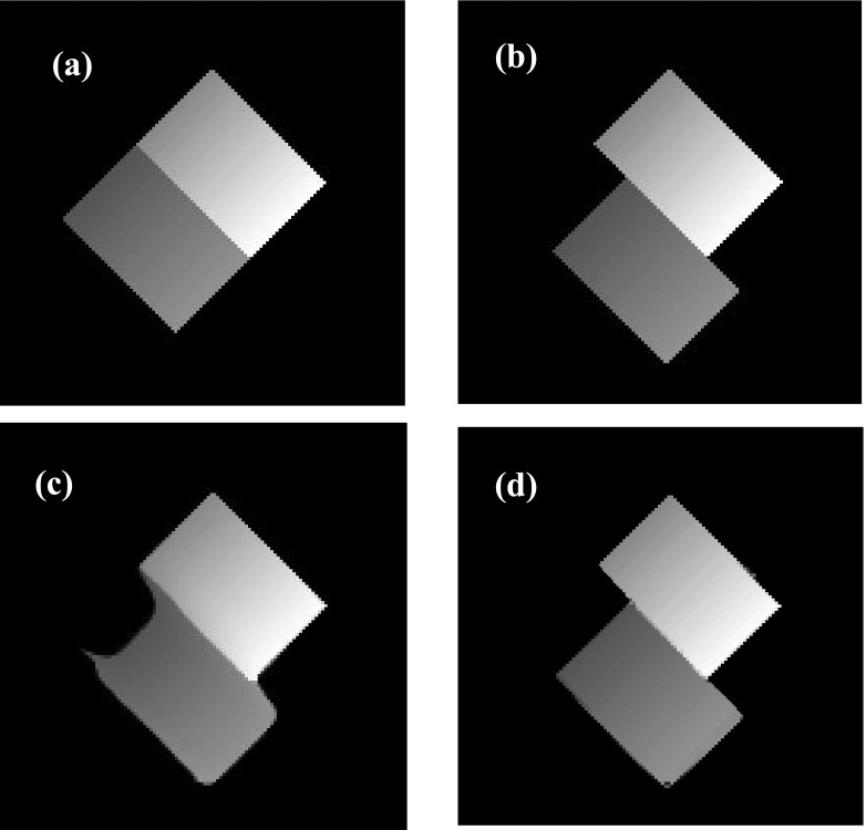
We also tested our algorithm effectiveness to compensate tube phantom sliding along other directions. Figure 3 shows the tube phantom results when it slides along 45° in the images. The results indicate that our algorithm is capable to avoid undesirable smoothing on the sliding boundary and achieves a more accurate deformation result.
FIG. 3.
(a) The initial phase for 45° sliding; (b) target phase for 45° sliding; (c) deformed initial phase without sliding consideration for 45°; (d) deformed initial phase with sliding consideration for 45°.
3.B. NCAT phantom
After the effectiveness of sliding motion constrained algorithm was testified by the sliding tube phantom, we continued to use the NCAT phantom to further evaluate the performance of our algorithm. 10 breathing phase of 4D NCAT were simulated with a respiration period of 4 s. The maximum diaphragm motion along superior–interior (SI) is 20 mm and the maximum chest anterior–posterior (AP) motion is 12 mm. The projections of 10 phases with 20 views per phase were used for the DVF estimation and 4D-CBCT reconstruction. The phantom image size is 256 × 256 × 150 with a voxel size of 2 × 2 × 2 mm3. The projection size is 300 × 240 × 20 view per phase with projection voxel size of 2 × 2 mm2.
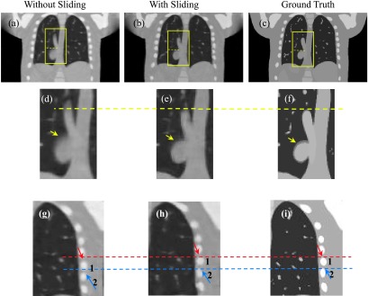
Figure 4 shows the 40% phase reconstructed images obtained with and without sliding motion constraint. As 40% phase has the largest respiration motion compared with the 0% phase, sliding motion would be obvious between the 2 phases. Hence we choose 40% phase to validate our algorithm. Figure 4(a) shows the 40% phase reconstructed images obtained without sliding motion constraint; Fig. 4(b) shows result with sliding constraint; Fig. 4(c) shows the corresponding ground truth image; Figs. 4(d)–4(f) are the ROIs where sliding motion happens. The ROIs show that the boundary border (indicated by the arrows) has been better kept with sliding consideration. Moreover, the vein (labeled by the yellow dotted line) is more accurately reconstructed with the sliding motion consideration. Figures 4(g)–4(i) show the ROIs around the lung and rib cage. These results further demonstrate that with sliding consideration [Fig. 4(g)], the rib positions match better to the ground truth [Fig. 4(i)] than that in the image without consideration sliding motion [Fig. 4(h)]. The ROI’s RE quantification results are also listed in Table I, with 6.7% for image with sliding motion consideration, and 8.5% for image without sliding consideration.
FIG. 4.
NCAT phantom results obtained with and without sliding motion compensation. (a) 40% phase reconstructed results without sliding constraint; (b) 40% phase reconstructed results with sliding constraint; (c) 40% phase ground truth; (d) ROI from (a); (e) ROI from (b); (f) ROI from (c); (g) lung–rib cage ROI without sliding motion constraint; (h) corresponding ROI with sliding motion consideration; (i) corresponding phantom ROI.
3.B.1. Dice coefficient
With the extracted lung boundaries from the ground truth and those obtained with/without sliding constraint, the 4D Dice coefficients with and without sliding constraint are summarized in Table II. The results illustrate that the lung boundary similarity obtained with sliding consideration is consistently larger than that without this consideration. The average Dice coefficient with sliding consideration was 0.988 compared with that of 0.955 without taking sliding into consideration. This indicates that the sliding consideration improved the organ contouring accuracy.
TABLE II.
4D Dice coefficients between NCAT phantom results obtained with/without sliding motion compensation.
| Phase index | 0% | 10% | 20% | 30% | 40% | 50% | 60% | 70% | 80% | 90% | Average Dice coefficient |
|---|---|---|---|---|---|---|---|---|---|---|---|
| Without sliding | 0.989 | 0.981 | 0.970 | 0.950 | 0.923 | 0.915 | 0.913 | 0.962 | 0.968 | 0.978 | 0.955 |
| With sliding | 0.998 | 0.998 | 0.991 | 0.990 | 0.989 | 0.986 | 0.979 | 0.986 | 0.988 | 0.986 | 0.990 |
3.B.2. Motion trajectory
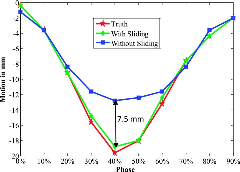
The 4D NCAT motion trajectory along the z-direction is extracted from the heart-to-lung sliding edge in the coronal views (see Fig. 4). The positions of front edges (labeled by the dotted line in the ROI in Fig. 4) are detected from a binary image by setting a uniform threshold on each phase ROI. The detected front edge positions are used to plot the motion trajectory. Figure 5 indicates that the trajectory extracted with sliding consideration matches with the ground truth much better than that without this consideration. Especially at phases with large motion such as 30%, 40%, and 50% phases, isotropic smoothing leads to obvious improper boundary smoothing. Table III further quantified the trajectory errors to illustrate how sliding consideration helped to improve the motion tracking accuracy. The errors with sliding consideration for each phase were all less than 1 mm, while the errors obtained without this consideration had much larger fluctuation. The RMSE and MaxE for all the 10 phases with sliding motion were 0.47 and 0.83 mm, respectively. These errors increased to 3.48 and 7.32 mm when the sliding motion was not taken into consideration during motion estimation.
FIG. 5.
z-axis heart motion trajectories extracted from the NCAT phantom ROI truth and the corresponding ROI images with and without sliding constraint.
TABLE III.
Motion trajectory error comparison.
| Phase index | 0% | 10% | 20% | 30% | 40% | 50% | 60% | 70% | 80% | 90% | RMSE and MaxE, mm |
|---|---|---|---|---|---|---|---|---|---|---|---|
| With sliding (mm) | 0.00 | 0.00 | 0.00 | 0.76 | 0.82 | 0.00 | 0.83 | 0.00 | 0.00 | 0.00 | 0.47/0.83 |
| Without sliding (mm) | 0.61 | 0.00 | 0.62 | 4.51 | 7.32 | 5.60 | 1.51 | 0.75 | 0.84 | 0.00 | 3.48/7.32 |
3.C. Patient study
Projections of two lung cancer patients were used to evaluate the proposed sliding constraint reconstruction algorithm. Under an IRB approved protocol (MD Anderson with IRB# 00-202), the patients were scanned with full fan mode for 4–6 min to acquire around 2000 projections, and these projections were sorted into 10 phases. When the number of average projections per phase was around 200, TV minimization reconstruction was performed to reconstruct the high quality 4D images. However, in a routine CBCT scan, the acquisition time is 1–2 min and the number of average projections per phase is about 60 after phase grouping. Our goal is to enhance 4D-CBCT acquired from a routine CBCT scan (1–2 min), where projections are undersampled using conventional reconstruction algorithms. The patient data obtained with long acquisition time offer the opportunity to reconstruct high quality reference images from adequate projections at each phase. These high-quality images were then considered as patient reference to evaluate the images reconstructed by SMEIR from downsampled projections (with the number of averaged projections per phase 40) to simulate a routine 1–2 min CBCT scan.
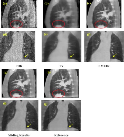
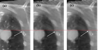
We then performed FDK, TV, SMEIR, and our sliding considered reconstruction for quantitative comparisons. Corresponding results are shown in Fig. 6. Figures 6(a)–6(c) and 6(g) show the sagittal view of the reconstructed results of the 1st patient via FDK, TV, SMEIR, and our sliding considered method, respectively. Figure 6(h) is the reference image reconstructed by TV from fully sampled projections. From Figs. 6(d)–6(f), 6(i), and 6(j) show the corresponding coronal view. In the sagittal views, the diaphragm boundary (labeled by the red ellipse) obtained via SMEIR method is slightly blurred if sliding is not considered. Moreover, in the coronal views of the lung boundary-to-heart corner (labeled by an arrow), the sliding results have the clearest boundary compared with the reference. Figure 7 shows a zoomed region around the lung–rib cage boundary for the 1st patient. The top edge of the rib (indicated by an arrow) in the reconstructed image with sliding motion modeling [Fig. 7(b)] is closer to the reference [Fig. 7(a)] than that in the image without considering sliding motion [Fig. 7(c)]. This example further demonstrates the benefit of sliding motion modeling.
FIG. 6.
Coronal and sagittal views of the first patient reconstruction using (a) and (d) FDK; (b) and (e) TV; (c) and (f) SMEIR without sliding; (g) and (i) SMEIR with sliding motion compensation; (h) and (j) reference image from fully sample projections.
FIG. 7.
(a) Reference image of the first patient; (b) reconstruction with sliding consideration; and (c) reconstruction without sliding consideration.
Table IV summarizes the RE of reconstructed images and the Dice coefficient of the lung boundary. The RE and the Dice coefficient indicate that sliding compensation achieves better reconstruction and lung contouring results.
TABLE IV.
RE and Dice coefficient comparison for patient study.
| Reconstruction | FDK | TV | SMEIR | Sliding result |
|---|---|---|---|---|
| RE (%) | 30.45 | 9.31 | 7.69 | 7.61 |
| Dice coefficient | 0.903 | 0.939 | 0.953 | 0.985 |
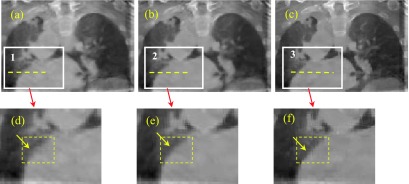
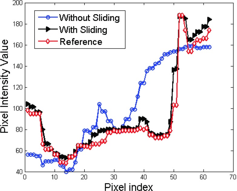
We continued to test our algorithm on the 2nd patient data. The results are shown in Figs. 8 and 9. Figure 8 shows the coronal views. The zoomed ROIs for the heart edge are also shown in Figs. 8(d)–8(f). The arrows in the yellow ROIs show that heart edge is better kept in Fig. 8(d) than that in Fig. 8(e) as compared to the reference Fig. 8(f). We plot the profiles along the dotted lines in ROIs 1, 2, and 3. And the results are shown in Fig. 9. The profile comparison results indicate that the sliding based cross boundary profile is much closer to the reference profile compared with SMEIR based profile.
FIG. 8.
Results (coronal views) for the second patient. (a) without sliding consideration; (b) with sliding consideration; (c) reference image; (d) zoomed ROI in (a); (e) zoomed ROI in (b); and (f) zoomed ROI in (c). (See color online version.)
FIG. 9.
Patient result profile comparison for results obtained with and without sliding consideration.
4. DISCUSSION AND CONCLUSION
In this work, we proposed a sliding motion-compensated 4D-CBCT reconstruction algorithm by modifying the DVF smoothing at the organ boundaries. Previous publications16–19 on sliding motion modeling mainly focused on the deformable image registration framework for two 3D volumetric images. In our work, we take sliding motion modeling into 4D-CBCT image reconstruction, where the DVF is estimated from 2D projections directly. We validated our algorithm with a digital sliding tube phantom, NCAT phantom, and two lung cancer patients.
In the proposed strategy, segmentation of lung is needed in order to identify the boundary region between lung and thoracic cage. Thus, the segmentation accuracy will influence the accuracy of motion estimation as well as the final reconstructed image. It is noted that the segmentation accuracy will also affect the Dice coefficient calculation. The lung segmentation was performed by a thresholding-based algorithm. For the NCAT phantom, it is easy to find a suitable threshold value for accurate segmentation of the lung due to its simple structure. The well extracted lung boundary facilitates the corresponding normal vectors to match well with the lung surface, and the sliding motion can be well corrected. Therefore the NCAT phantom based results is good evidence to demonstrate our method’s efficiency. While for the patient data with abundant noise and artifacts, it is not straightforward to find a good threshold that is capable to ideally extract the lung boundary everywhere in the image due to its complex structure. Careful tuning of the threshold in a trial-and-error style was performed to decide the threshold for all the 10 phase lung boundaries in this work.
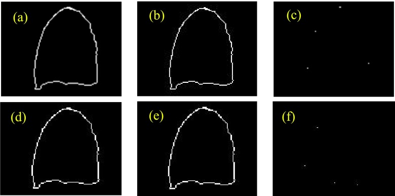
As our reconstruction is a iterative process, the corresponding lung should be also segmented with each iteration to update the lung surface. However, this breaks the automatic iterative reconstruction too frequently as currently we are using a semi-automatic segmentation. Practically, we only updated the lung surface every 5 reconstruction iterations instead of every 1 iteration as the change of boundary is not dramatic between the two successive iterations. As shown in Fig. 10, there is no visible difference of lung boundaries when segmentation is performed every 5 iterations or 1 iteration. Therefore, for practical consideration, we performed the lung segmentation every 5 reconstruction iterations in this work.
FIG. 10.
Lung segmentation accuracy comparison: contour updating every 1 reconstruction iteration vs every 5 reconstruction iterations. (a) with updating by every 1 reconstruction iteration, the contour obtained after 5 reconstruction iterations; (b) with updating by every 5 reconstruction iterations, the contour obtained after 5 reconstruction iterations; (c) contour difference between (a) and (b); (d) with updating by every 1 reconstruction iteration, the contour obtained after 10 reconstruction iterations; (e) with updating by every 5 reconstruction iteration, the contour obtained after 10 reconstruction iterations; (f) contour difference between (d) and (e).
Compared to the NCAT phantom results, our patient results only show limited improvements. One possible reason is that accurate sliding modeling depends on accurate lung boundary segmentation. Compared to the phantoms, it is more challenging to obtain accurate segmentation in patient CBCT due to its complex structure and shading artifacts. In this work, a thresholding-based method was used to segment the lung. While the threshold was fine-tuned, the accuracy for lung segmentation was still limited. More advanced segmentation algorithms28,29 can be employed to improve the accuracy of lung boundary segmentation. Another possible reason is that the sliding motion between lung and thoracic cage is small for the patients studied in this work. While the range of diaphragm motion was 8 and 14 mm for patients 1 and 2, respectively, the motion difference between the corner of diaphragm and adjacent thoracic cage (i.e., sliding motion) was only 3 and 5 mm for patients 1 and 2, respectively.
Compared to the original SMEIR algorithm without modeling sliding motion, the requirement of lung segmentation in the proposed algorithm will compromise the clinical workflow and efficiency. More advanced automatic segmentation algorithms28,29 need to be adopted to improve the segmentation accuracy and workflow efficiency. Furthermore, due to the modified design of the penalty term, the optimization for minimizing Eq. (3) is also affected. While the convergence of the presented algorithm is similar to the original SMEIR algorithm where 200 total iterations in the DVF estimation are adequate to achieve good convergence, longer computation time is needed in the present algorithm. The computation time for one iteration during the DVF optimization also increases from 22 s of the original SMEIR to 25 s for the presented algorithm to reconstruct an image of size 200 × 200 × 150. Currently, DVFs for each phase were estimated sequentially and we partially implemented the algorithm on a GPU card (Geforce GTX 980, NVIDA, Santa Clara, CA). Only the forward projection at one view angle was simultaneously calculated on GPU. The computation efficiency can be improved by (1) full GPU implementation and (2) running DVF estimation for different phases in a parallel fashion on multiple GPU cards.
In summary, we have proposed a sliding motion-compensated scheme for accurate 4D-CBCT reconstruction. The segmented lung boundary’s normal vectors are capable to guide the adaptive local DVF smoothing. Hence lung’s local anisotropic sliding motion is capable to be captured, leading to more accurate reconstruction and motion tracking. While further patient studies are needed, this algorithm could improve the performance of 4D-CBCT in image-guided radiation therapy.
ACKNOWLEDGMENTS
We acknowledge funding supports from the American Cancer Society (Grant No. RSG-13-326-01-CCE), from the U.S. National Institutes of Health (Grant No. R01 EB020366), from the Cancer Prevention and Research Institute of Texas (Grant No. RP130109), and from Varian Medical System also. We acknowledge Dr. Tinsu Pan from M.D. Anderson Cancer Center for sharing patient data in the evaluation study.
CONFLICT OF INTEREST DISCLOSURE
The authors have no COI to report.
REFERENCES
- 1.Lu J., Guerrero T. M., Munro P., Jeung A., Chi P. C., Balter P., Zhu X. R., Mohan R., and Pan T., “Four-dimensional cone beam CT with adaptive gantry rotation and adaptive data sampling,” Med. Phys. (9), 3520–3529 (2007). 10.1118/1.2767145 [DOI] [PubMed] [Google Scholar]
- 2.Wang J. and Gu X., “High-quality four-dimensional cone-beam CT by deforming prior images,” Phys. Med. Biol. (2), 231–246 (2013). 10.1088/0031-9155/58/2/231 [DOI] [PubMed] [Google Scholar]
- 3.Bergner F. F., Berkus T., Oelhafen M., Kunz P., Pan T., and Kachelriess M., “Autoadaptive phase-correlated (AAPC) reconstruction for 4D CBCT,” Med. Phys. (12), 5695–5706 (2009). 10.1118/1.3260919 [DOI] [PMC free article] [PubMed] [Google Scholar]
- 4.Zhang Y., Yin F. F., Segars W. P., and Ren L., “A technique for estimating 4D-CBCT using prior knowledge and limited-angle projections,” Med. Phys. (12), 121701 (12pp.) (2013). 10.1118/1.4825097 [DOI] [PubMed] [Google Scholar]
- 5.Dang J., Luo O., Gu X., and Wang J., “Deformation vector fields (DVF)-driven image reconstruction for 4D-CBCT,” J. X-Ray Sci. Technol. (1), 11–23 (2015). 10.3233/XST-140466 [DOI] [PubMed] [Google Scholar]
- 6.Vergalasova I., Cai J., and Yin F. F., “A novel technique for markerless, self-sorted 4D-CBCT: Feasibility study,” Med. Phys. (3), 1442–1451 (2012). 10.1118/1.3685443 [DOI] [PMC free article] [PubMed] [Google Scholar]
- 7.Zhang Y., Yin F. F., Pan T., Vergalasova I., and Ren L., “Preliminary clinical evaluation of a 4D-CBCT estimation technique using prior information and limited-angle projections,” Radiother. Oncol. (1), 22–29 (2015). 10.1016/j.radonc.2015.02.022 [DOI] [PMC free article] [PubMed] [Google Scholar]
- 8.Dang J., Gu X., Pan T., and Wang J., “A pilot evaluation of a 4-dimensional cone-beam computed tomographic scheme based on simultaneous motion estimation and image reconstruction,” Int. J. Radiat. Oncol., Biol., Phys. (2), 410–418 (2015). 10.1016/j.ijrobp.2014.10.029 [DOI] [PubMed] [Google Scholar]
- 9.Kida S., Saotome N., Masutani Y., Yamashita H., Ohtomo K., Nakagawa K., Sakumi A., and Haga A., “4D-CBCT reconstruction using MV portal imaging during volumetric modulated arc therapy,” Radiother. Oncol. (3), 380–385 (2011). 10.1016/j.radonc.2011.08.047 [DOI] [PubMed] [Google Scholar]
- 10.Vergalasova I., Cai J., Giles W., Segars W. P., and Yin F. F., “Evaluation of the effect of respiratory and anatomical variables on a Fourier technique for markerless, self-sorted 4D-CBCT,” Phys. Med. Biol. (20), 7239–7259 (2013). 10.1088/0031-9155/58/20/7239 [DOI] [PMC free article] [PubMed] [Google Scholar]
- 11.Jia X., Tian Z., Luo Y., Sonke J. J., and Jiang S. B., “Four-dimensional cone beam CT reconstruction and enhancement using a temporal nonlocal means method,” Med. Phys. (9), 5592–5602 (2012). 10.1118/1.4745559 [DOI] [PMC free article] [PubMed] [Google Scholar]
- 12.Shieh C. C., Kipritidis J., O’Brien R. T., Cooper B. J., Kuncic Z., and Keall P. J., “Improving thoracic four-dimensional cone-beam CT reconstruction with anatomical-adaptive image regularization (AAIR),” Phys. Med. Biol. (2), 841–868 (2015). 10.1088/0031-9155/60/2/841 [DOI] [PMC free article] [PubMed] [Google Scholar]
- 13.Gao H., Ruijiang L., Yuting L., and Lei X., “4D cone beam CT via spatiotemporal tensor framelet,” Med. Phys. (11), 6943–6946 (2012). 10.1118/1.4762288 [DOI] [PMC free article] [PubMed] [Google Scholar]
- 14.Wang J. and Gu X., “Simultaneous motion estimation and image reconstruction (SMEIR) for 4D cone-beam CT,” Med. Phys. (10), 101912 (11pp.) (2013). 10.1118/1.4821099 [DOI] [PubMed] [Google Scholar]
- 15.Snoke J. J., Zijp L., Remeijer P., and van Herk M., “Respiratory correlated cone beam CT,” Med. Phys. (4), 1176–1186 (2005). 10.1118/1.1869074 [DOI] [PubMed] [Google Scholar]
- 16.Wu Z., Rietzel E., Boldea V., Sarrut D., and Sharp G. C., “Evaluation of deformable registration of patient lung 4DCT with subanatomical region segmentations,” Med. Phys. (2), 775–781 (2008). 10.1118/1.2828378 [DOI] [PubMed] [Google Scholar]
- 17.Vandemeulebroucke J., Bernard O., Rit S., Kybic J., Clarysse P., and Sarrut D., “Automated segmentation of a motion mask to preserve sliding motion in deformable registration of thoracic CT,” Med. Phys. (2), 1006–1015 (2012). 10.1118/1.3679009 [DOI] [PubMed] [Google Scholar]
- 18.Schmidt-Richberg A., Werner R., Handels H., and Ehrhardt J., “Estimation of slipping organ motion by registration with direction-dependent regularization,” Med. Image Anal. (1), 150–159 (2012). 10.1016/j.media.2011.06.007 [DOI] [PubMed] [Google Scholar]
- 19.Risser L., Vialard F. X., Baluwala H. Y., and Schnabel J. A., “Piecewise-diffeomorphic image registration: Application to the motion estimation between 3D CT lung images with sliding conditions,” Med. Image Anal. (2), 182–193 (2013). 10.1016/j.media.2012.10.001 [DOI] [PubMed] [Google Scholar]
- 20.Zhong Z., Gu X., Mao W., and Wang J., “4D cone-beam CT reconstruction using multi-organ meshes for sliding motion modeling,” Phys. Med. Biol. (3), 996–1020 (2016). 10.1088/0031-9155/61/3/996 [DOI] [PMC free article] [PubMed] [Google Scholar]
- 21.Han G., Liang Z., and You J., “A fast ray-tracing technique for TCT and ECT studies,” IEEE Nucl. Sci. Symp. Conf. Rec. , 1515–1518 (1999). 10.1109/nssmic.1999.842846 [DOI] [Google Scholar]
- 22.Sidky E. Y. and Pan X., “Image reconstruction in circular cone-beam computed tomography by constrained, total-variation minimization,” Phys. Med. Biol. (17), 4777–4807 (2008). 10.1088/0031-9155/53/17/021 [DOI] [PMC free article] [PubMed] [Google Scholar]
- 23.Pace D. F., Aylward S. R., and Niethammer M., “A locally adaptive regularization based on anisotropic diffusion for deformable image registration of sliding organs,” IEEE Trans. Med. Imaging (11), 2114–2126 (2013). 10.1109/TMI.2013.2274777 [DOI] [PMC free article] [PubMed] [Google Scholar]
- 24.Yushkevich P. A., Piven J., Hazlett H. C., Smith R. G., Ho S., Gee J. C., and Gerig G., “User-guided 3D active contour segmentation of anatomical structures: Significantly improved efficiency and reliability,” Neuroimage (3), 1116–1128 (2006). 10.1016/j.neuroimage.2006.01.015 [DOI] [PubMed] [Google Scholar]
- 25.Thirion J. P., “Image matching as a diffusion process: An analogy with Maxwell’s demons,” Med. Image Anal. (3), 243–260 (1998). 10.1016/S1361-8415(98)80022-4 [DOI] [PubMed] [Google Scholar]
- 26.Kroon D.-J., Multimodality non-rigid demon algorithm image registration, last accessed May 16, 2016, http://www.mathworks.com/matlabcentral/fileexchange/21451-multimodality-non-rigid-demon-algorithm-image-registration.
- 27.Vercauteren T., Pennec X., Perchant A., and Ayache N., “Non-parametric diffeomorphic image registration with the demons algorithm,” Med. Image Comput. Comput. Assist. Interv. (Pt 2), 319–326 (2007). [DOI] [PubMed] [Google Scholar]
- 28.van Rikxoort E. M., de Hoop B., Viergever M. A., Prokop M., and van Ginneken B., “Automatic lung segmentation from thoracic computed tomography scans using a hybrid approach with error detection,” Med. Phys. (7), 2934–2947 (2009). 10.1118/1.3147146 [DOI] [PubMed] [Google Scholar]
- 29.Soleymanpour E., Pourreza H. R., Ansaripour E., and Yazdi M. S., “Fully automatic lung segmentation and rib suppression methods to improve nodule detection in chest radiographs,” J. Med. Signals Sens. (3), 191–199 (2011). [PMC free article] [PubMed] [Google Scholar]


