Improved prediction of antibody V_L–V_H orientation

Abstract

Antibodies are important immune molecules with high commercial value and therapeutic interest because of their ability to bind diverse antigens. Computational prediction of antibody structure can quickly reveal valuable information about the nature of these antigen-binding interactions, but only if the models are of sufficient quality. To achieve high model quality during complementarity-determining region (CDR) structural prediction, one must account for the V_L–V_H orientation. We developed a novel four-metric V_L–V_H orientation coordinate frame. Additionally, we extended the CDR grafting protocol in RosettaAntibody with a new method that diversifies V_L–V_H orientation by using 10 V_L–V_H orientation templates rather than a single one. We tested the multiple-template grafting protocol on two datasets of known antibody crystal structures. During the template-grafting phase, the new protocol improved the fraction of accurate V_L–V_H orientation predictions from only 26% (12/46) to 72% (33/46) of targets. After the full RosettaAntibody protocol, including CDR H3 remodeling and V_L–V_H re-orientation, the new protocol produced more candidate structures with accurate V_L–V_H orientation than the standard protocol in 43/46 targets (93%). The improved ability to predict V_L–V_H orientation will bolster predictions of other parts of the paratope, including the conformation of CDR H3, a grand challenge of antibody homology modeling.

Introduction

Antibodies are important immune molecules with high commercial value and therapeutic interest because of their ability to bind diverse antigens, from small molecules and short peptides to full-length proteins. Antibodies' binding diversity is a function of their hypervariable F_V domains, each consisting of two immunoglobulin domains: V_L and V_H. The antigen-binding site (paratope) is located at six loops near the V_L–V_H interface, known as complementarity-determining regions, or CDRs.

Many structural studies of the F_V have focused on the conformation of the CDRs, particularly CDR H3 (Al-Lazikani et al., 1997; North et al., 2011; Wang et al., 2013; Weitzner et al., 2015; Xu et al., 2015). Because the CDRs are attached to the framework of the V_L and V_H domains, any change in the relative orientation of the V_L and V_H domains will propagate to change the CDRs' relative orientation, and therefore, the shape of the paratope. Failing to account for the V_L–V_H orientation during CDR or paratope structure prediction dramatically hinders the quality of the output models, and recent evaluation found the V_L–V_H orientation to be a limiting factor in antibody structure prediction (Weitzner et al., 2014).

Abhinandan and Martin (2010) were the first to codify a metric for measuring the V_L–V_H orientation. They defined the packing angle as a torsional angle between the primary axes of the V_L and V_H domains. Among the ∼500 F_V crystal structures they examined, packing angle differed by as much as 30°. Chailyan et al. (2011) defined V_L–V_H orientation differently, via clustering. The resulting description was limited in scope: only two distinct orientational clusters and a distinct singleton were found; however, a number of key residues were found to correlate with the orientational clusters, indicating that V_L–V_H orientation may be predictable from sequence.

The Second Antibody Modeling Assessment (AMA-II) measured the ability of several computational antibody structural prediction methods to capture native V_L–V_H orientation in a blind prediction challenge. Two metrics were used to evaluate the antibody orientations generated in AMA-II: (i) an analogue to RMSDvariable as described by Sela-Culang et al. (2012), and (ii) the tilt angle as described in Almagro et al. (2014). While these measures encode more orientational information than the Abhinandan–Martin packing angle, both are pairwise difference metrics rather than absolute ones. A geometrically complete, absolute measure of V_L–V_H orientation, ABangle, was published by Dunbar et al. (2013). ABangle is composed of one torsional angle, four plane angles and one distance, representing the six degrees of freedom of the two-body V_L–V_H complex. The ABangle measure was applied in a study to predict V_L–V_H orientation. In tests on the AMA-II antibody set, the authors predicted ABangle metrics corresponding to an average RMSD of misorientation of 0.50 Å, performing better than the average competitor (0.63 Å), beating the average in 9 of 11 targets (Bujotzek et al., 2015).

RosettaAntibody is an application for blind prediction of antibody structure (Sivasubramanian et al., 2009; Weitzner et al., 2014). RosettaAntibody operates in two phases: (i) template selection and grafting, wherein known antibody structure fragments are combined to create a coarse-grained model, and (ii) structure refinement, which uses Monte Carlo perturbations with minimization to remodel the CDR H3 loop, refine all CDR loops, and redock the V_L and V_H domains.

Until recently, RosettaAntibody's efficacy in predicting native V_L–V_H orientations had only been investigated implicitly by measuring RMSD values across all F_V residues. During the Second Antibody Modeling Assessment (AMA-II), RosettaAntibody's orientation predictions were evaluated explicitly, comparing the packing angles of the Rosetta models to those of their corresponding crystal structures (Weitzner et al., 2014). RosettaAntibody compared favorably in most respects to the competing protocols, producing two sub-Ångstrom H3 models and achieving the best H3 model in four targets. However, V_L–V_H orientation was a weakness, as RosettaAntibody created a structure with sub-Ångstrom cross-domain RMSD for only 5 of 11 targets. V_L–V_H orientation prediction for targets with uncommon packing angles was particularly poor: all three targets with a packing angle more than 1 SD removed from the database average were predicted incorrectly.

In this article, we developed a novel four-metric V_L–V_H orientation coordinate frame, which we called Light–Heavy Orientational Coordinates (LHOC). Additionally, we extended the RosettaAntibody protocol with a new method to diversify V_L–V_H orientations by grafting multiple templates. We tested the new RosettaAntibody protocol on two datasets of known antibody crystal structures: a 46-member high-resolution antibody set, and the 11-member AMA-II dataset. We compared the performance of the new RosettaAntibody against the previous version, as well as against the ABangle method for predicting V_L–V_H orientation.

Materials and methods

Orientational coordinates framework calculation

The four coordinates used to describe V_L–V_H orientation (α, δ_ID, θ_L, and θ_H) are defined from a common framework of four non-atomic points at the V_L–V_H interface (Fig. 1). Point 2 is located at the center of a conserved pair of beta strands in the V_L framework; it is defined as the centroid of the C_α coordinates of residues L35–L38 and L85–L88 using Chothia numbering (Al-Lazikani et al., 1997). Point 3 is the V_H counterpart to Point 2, defined as the centroid of the C_α coordinates of residues H36–H39 and H89–H92, Chothia numbering. Point 1 is located nearer the CDRs than Point 2, along the first principal component line of the coordinate set used to calculate point 2. Point 4 is the V_H counterpart to point 1.

Fig. 1.

Orientational coordinate (LHOC) definition. (a) F_V structure showing light chain (cyan), heavy chain (pink) and the key beta strands for defining the LHOC framework (Chothia numbering: L35-L38 and L85-L88 in blue and H36-H39 and H89-H92 in red, see ‘Materials and Methods’ for details). The inset shows the placement of the four points, which form the basis of the LHOC framework. (b) Packing angle, α, is the dihedral angle between points 1, 2, 3 and 4. (c) Interdomain distance, δ_ID, is the distance between Points 2 and 3. (d) L-opening angle, θ_L, is the plane angle between Points 1, 2 and 3. (e) H-opening angle, θ_H, is the plane angle between Points 2, 3 and 4.

All coordinates were calculated with a Rosetta implementation of the above framework. α is defined in the same manner as Abhinandan and Martin (2010); specifically, it is defined as the dihedral angle between points 1, 2, 3 and 4. δ_ID is defined as the distance between Points 2 and 3. θ_L is defined as the plane angle between Points 1, 2, and 3. θ_H is defined as the plane angle between Points 2, 3 and 4.

Orientational Coordinate Distance measurement

Orientational Coordinate Distance (OCD) is calculated as:

$$\text{OCD}={\sum }_{i=\{a,{\delta }_{\mathrm{ID},}{\theta }_{\mathrm{L}},{\theta }_{\mathrm{H}}\}}\left(\frac{x_{i,\mathrm{A}}-x_{i,\mathrm{B}}}{{\sigma }_{i,d\mathrm{B}}}\right),$$

where x_i,A and x_i,B represent the value of LHOC metric i of structure A and structure B, respectively, and σ_i,dB represents the standard deviation of the Gaussian distribution best fit to the database distribution of LHOC metric i. The four values for i are α, δ_ID, θ_L and θ_H. OCD is dimensionless.

RosettaAntibody command lines

The new MT protocol, part of the Rosetta software package, is available free of charge for academic and nonprofit use at www.rosettacommons.org. The code used to generate data in this article is available starting from release revision 57, deposited 21 May 2015. The MT protocol is available on the ROSIE public Web server (rosie.graylab.jhu.edu, Lyskov et al., 2013) as an option of the Antibody homology modeling protocol.

To create the grafted structures, the following command line was used. The homolog_exclusion argument should be 99 when performing blind predictions, and 80 when evaluating algorithm performance on a known set.

antibody.py --both-chains < FASTA file> --relax

  --homolog_exclusion=<99||80>

  --multi-template-grafting --number-of-templates 10

  --light_heavy-multi-graft

  --filter-by-orientational-distance = 1

  --orientational-distance-cutoff 0.5

To create the candidate structures, the following command line was used for each grafted structure. abH3.flags is a text file containing the set of option flags for a standard RosettaAntibody run. The cter_constraint file is a two-line text file containing two atomic constraints; it is generated automatically by the previous command line. The grafted structure is one of 10 models generated by the previous command line. The -nstruct argument should be 1000 for the first grafted structure, and 200 for the other nine models.

antibody_H3.linuxgccrelease @abH3.flags

  -s < grafted structure, 1 of 10> -nstruct <200||1000>

  -constraints:cst_file < cter_constraint file>

Preparation of antibody database set

The RosettaAntibody database consists of 1040 antibody F_V crystal structures culled from the Protein Data Bank using the methods described by Sivasubramanian et al. (2009). One outlier antibody (1MCO) has an interdomain distance of 19.6 Å, farther removed from the second-largest interdomain distance than the second-largest is from the smallest. This antibody is highly irregular, with the F_Ab–F_C hinge region deleted (Guddat et al., 1993), explaining the unnaturally large interdomain distance; this antibody was consequently removed from analyses of the RosettaAntibody database.

Preparation of antibody benchmark sets

A high-resolution antibody set was compiled from the PyIgClassify database (Adolf-Bryfogle et al., 2015). A series of restrictions was placed on the structures: a maximum resolution of 2.5 Å, a maximum R value of 0.2, a maximum B-factor of 80.0 Ų for each atom in the structure, an asymmetric unit containing only one copy of the F_V, a CDR H3 loop length between 9 and 20 residues, a human or mouse species tag and no non-canonical or modified amino acid residues. Additionally, the set was filtered to remove antibodies with identical sequences in any of the heavy-chain CDR loops. Of the resultant 49 structures, 3 (1X9Q, 2W60, 3IFL) were eliminated because of challenges presented in sequence misalignment or numbering (e.g. 1X9Q is missing highly conserved heavy-chain residues C92 and W103). The Second Antibody Modeling Assessment (AMA-II) antibody set consists of the 11 antibodies described in Almagro et al. (2014).

Results

A new V_L–V_H coordinate frame

To describe the geometry of antibody V_L–V_H orientation, we developed a new coordinate frame (Fig. 1) as an extension of the packing angle described by Abhinandan and Martin (2010). Three vectors compose the Abhinandan–Martin framework: two primary axis vectors, one each drawn through V_L and V_H, and a third vector linking the axis vectors tail-to-tail across the V_L–V_H interface. The Abhinandan–Martin packing angle (α) is defined as the apparent angle between the V_L and V_H vectors as seen when looking down the connecting line from V_H to V_L (Fig. 1b). The packing angle metric captures the set of V_L–V_H relative positions in which the V_L and V_H domains twist past each other, broadening or contracting the paratope. Figure 2 shows, however, that antibodies with identical α will not necessarily superimpose, and in practice, they often do not. This structural ambiguity is an inherent limitation of the α metric. Therefore, we sought a more complete description of the V_L–V_H orientation.

Fig. 2.

Two RosettaAntibody F_V models of AMA-II target 5 (PDB ID 4M6M) with equivalent values of the packing angle. Structures have light chains (black) superimposed. Heavy chains are shown in red and blue. CDR residues (Chothia definition) are omitted for clarity.

To capture more of the V_L–V_H orientation degrees of freedom, we repurposed the Abhinandan–Martin packing angle vector framework to define the other metrics: an interdomain distance (δ_ID) and two plane angles, L-opening angle (θ_L) and H-opening angle (θ_H). δ_ID is defined as the length of the linking vector (Fig. 1c). θ_L and θ_H are defined as the plane angle between the linking vector and the V_L and V_H vectors, respectively (Fig. 1d and e). Together, we refer to the four coordinates (α, δ_ID, θ_L and θ_H) as the LHOC.

For LHOC to be a non-redundant coordinate frame and more descriptive than the Abhinandan–Martin packing angle, each coordinate must capture some component of V_L–V_H orientational diversity that is sufficiently independent from the components captured by other coordinates. To evaluate the effectiveness of the LHOC coordinate frame, we calculated the LHOC metrics for each antibody in a curated set of 1040 antibody F_V crystal structures, representing a high- and medium-resolution (≤3.5 Å) subset of all antibodies in the Protein Data Bank.

Figure 3 shows distributions for each of the four LHOC metrics across all antibodies in the database. All three angle distributions are approximately Gaussian. Consistent with the prior use of packing angle to solely define V_L–V_H orientation (Abhinandan and Martin, 2010; Almagro et al., 2014), the α distribution is the largest component of diversity in V_L–V_H orientation, with a range of nearly 35° [mean (μ) = −52.3°, standard deviation (σ) = 3.9°, minimum = −70.9°, maximum = −36.7°]. The two LHOC plane angle distributions each show a range approximately half as large as the α distribution. The θ_L distribution has a range of about 15° (μ = 97.2°, σ = 1.9°, min = 89.3°, max = 104.4°), while the θ_H distribution has a range of about 20° (μ = 99.4°, σ = 2.6°, min = 87.9°, max = 108.1°). The δ_ID distribution is also approximately Gaussian, but with a long right tail. While the bulk of the distribution, 1030 of 1040 structures, lies between 13.5 and 15.5 Å, 9 of the 10 remaining structures have a δ_ID between 15.5 and 16.5 Å.

Fig. 3.

Histograms of each of the four LHOC metrics across the 1,040 structures in the Rosetta antibody database. Histogram bin widths are 1° for packing angle, α, (a), 0.1 Å for interdomain distance, δ_ID, (b), and 0.5° for plane angles, θ_L and θ_H, (c and d). Kernel density estimates of each distribution are shown as curves over the histograms.

To test the independence of the four LHOC metrics, we plotted all pairwise distributions of metrics for the database antibodies, shown in Supplementary data, Figure S1. Five of the six pairs of metrics show no correlation (r² ≤ 0.01), with approximately 2D-Gaussian distributions. The remaining pair, θ_H and δ_ID, show a small degree of correlation (r² = 0.16); antibodies with larger-than-average δ_ID tend to also have larger-than-average θ_H. Such a correlation could arise because the hinge of the θ_H definition differs from the physical hinge about which the V_L–V_H orientation actually varies between antibodies. If the physical hinge were upstream of the θ_H hinge, a naturally ‘open’ antibody would have both a larger θ_H and a larger δ_ID. In this case, one would also expect the antibody to also have a larger θ_L, as it is effectively a mirror image of θ_H; however, there is no correlation seen between δ_ID and θ_L, suggesting that the mathematical and physical hinges are in a similar place. This implies that the correlation between θ_H and δ_ID is not due to misplacement of the LHOC framework, nor a redundant selection of coordinates to include in LHOC.

The four-coordinate nature of the LHOC framework allows it to describe more facets of V_L–V_H orientation than α alone, but it requires a combination metric to simplify the difference to one dimension. Therefore, we defined the OCD by summing the squared z-score deviations in each of the four LHOC base metrics (see ‘Materials and methods’ for details). Figure 4a shows that a pair of antibodies with an OCD of 1.0 or less superimpose closely, and Figure 4b shows that a pair of antibodies with an OCD of 2.0 or greater are clearly distinct.

Fig. 4.

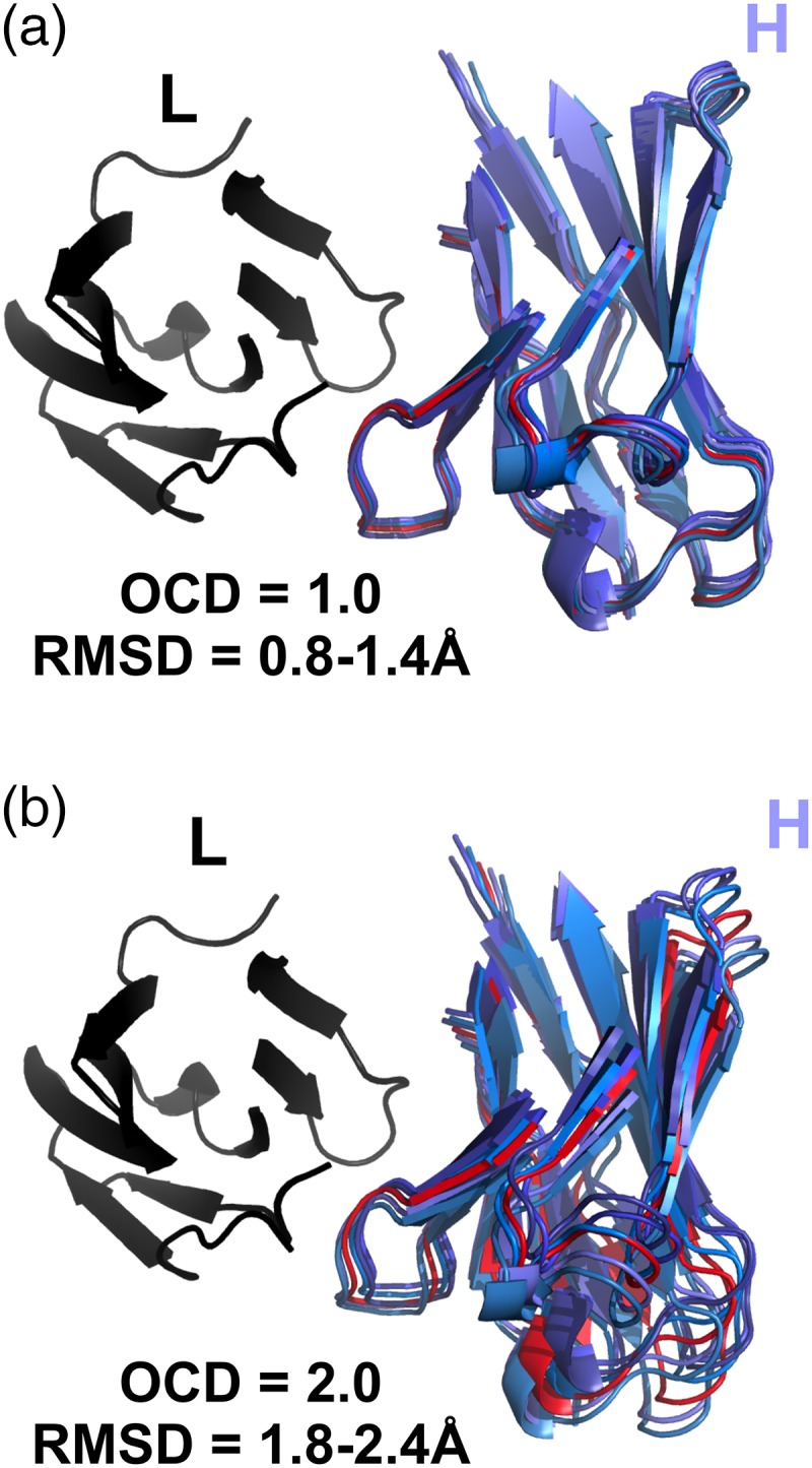
Comparison of five RosettaAntibody F_V models (blues) with 1.0 OCD (a) and 2.0 OCD (b) to a reference antibody F_V structure (red). Structures have light chains (black) superimposed. CDR residues (Chothia definition) are omitted for clarity.

Because changes in the different LHOC metrics exert different lever-arm effects on the antibody domains, and because the contributions to OCD can be dominated by a large variation in one or two LHOC metrics, two antibody pairs with the same OCD will not necessarily have the same RMSD between them. For example, two antibodies with a 3.0 OCD due only to a difference in packing angle will have a much larger RMSD than two antibodies with a 3.0 OCD due only to a difference in interdomain distance. Nonetheless, OCD and RMSD are loosely correlated: as shown in Supplementary data, Figure S2, two structures with a high OCD tend to have a high RMSD as well. An OCD of 2.0 is roughly equivalent to an RMSD of 1 Å, although most 2.0 OCD structure pairs will have a larger RMSD due to intradomain variations.

V_L–V_H orientation prediction in Rosetta

With the OCD metric, we next sought to test the efficacy of RosettaAntibody at predicting correct V_L–V_H orientations. A preliminary examination of the RosettaAntibody candidate structures for one of the AMA-II targets with an incorrect V_L–V_H orientation prediction revealed that a wide range of V_L–V_H orientations were sampled by docking moves during the structure refinement phase—so wide, in fact, that nearly the entire database distribution is spanned in all coordinates. However, the lowest-scoring candidate structures, and thus, the ones selected as final models, had orientations quite similar to the starting point of the refinement trajectories, i.e. the grafted structure. To examine how the starting point biases the output orientations, we launched refinement trajectories from grafted structures with alternate V_L–V_H orientations. Figure 5 shows the orientation distributions of candidate structures generated by these runs. In each trajectory, there is a visible well in which low-scoring candidate structures tend to have orientations matching their individual grafted structures rather than converging to the native orientation. These data suggest that the refinement phase of RosettaAntibody has an effective limit on how far it can alter the V_L–V_H orientation. While more orientationally distant structures can be sampled, these structures do not resemble natural antibodies, as evidenced by their high scores. This behavior is beneficial when the grafted structure has a native V_L–V_H orientation, but in the general case, it indicates an inadequate search.

Fig. 5.

H-opening angle, θ_H, distributions among candidate structures generated by RosettaAntibody from three different starting grafted structures with different V_L–V_H orientations. (a) Plots of θ_H versus score, showing scoring funnels for each of the three runs in a different color, with the grafted structure θ_H marked by a matching-color triangle below the x-axis. (b) Histograms and kernel density estimates for each of the three runs in a different color, with the θ_H of each grafted starting structure marked as in (a).

To attempt to produce low-scoring candidate structures near the native V_L–V_H orientation, we created a new RosettaAntibody grafting protocol that runs several trajectories rather than a single trajectory. A flowchart description of the protocol, called multiple-template (MT) grafting, is shown in Figure 6 in the context of the previous RosettaAntibody protocol, henceforth described as single-template (ST) grafting. Instead of creating only a single-grafted structure during the first phase of RosettaAntibody, MT creates 10 grafted structures from the 10 best-matching (by BLAST alignment) V_L–V_H orientation templates. Additionally, to diversify the grafted structures, we enforce a minimum OCD cutoff value of 0.5 between all orientation template pairs, rejecting candidate templates with a lower OCD to any of the 10 and replacing them with the next-best BLAST match. The number 10 and the 0.5 OCD cutoff were selected to capture a near-native V_L–V_H orientation in all targets in our calibration set, the 11 AMA-II antibodies, while minimizing the number of redundant templates. Each grafted structure is refined in multiple independent RosettaAntibody refinement runs to create a pool of candidate structures: 1000 from the shared ST/MT grafted structure, and 200 each from the remaining 9 MT grafted structures.

Fig. 6.

Flow chart for the RosettaAntibody protocol. The grafting phase is shown in blue and pink, above the solid gray line, while the refinement phase is shown in green and gold, below the solid gray line. Steps from the standard ST grafting protocol are colored in blue and green. New steps added to create the MT grafting protocol are colored in pink and gold and enclosed in the dashed gray box; the blue/green ST steps are also part of the MT protocol.

To evaluate the sampling efficacy of MT grafting, we compared the performance of ST and MT RosettaAntibody on a benchmark set of 46 high-resolution, manually curated antibody crystal structures from the Protein Data Bank (PDB) (Berman et al., 2000). Figure 7 shows the pairwise comparisons of OCD values between the ST and MT predictions for all targets. In the grafting phase of RosettaAntibody, the ST V_L–V_H orientation prediction was within 2.0 OCD of the native in only 26% (12/46) of targets. The MT predictions nearly tripled this, with the best match among the MT predictions within 2.0 OCD of native in 72% (33/46) of targets. Additionally, of the remaining 13 targets, 10 showed an improved OCD to native in their best MT prediction versus the ST prediction.

Fig. 7.

Comparison of V_L–V_H orientation prediction performance between MT RosettaAntibody and ST RosettaAntibody after the grafting stage for the 46 members of the benchmark set. The OCD between the native structure and the ST post-grafting stage structure is plotted against the lowest OCD between the native and any of the 10 MT post-grafting stage structures. Targets where the best MT structure is the same as the ST structure appear on the x = y line also plotted. Targets where the best MT structure has a closer OCD to native than the ST structure are above the x = y line. MT success cases (OCD ≤ 2.0) are found to the left of the vertical OCD = 2.0 line, while MT failures (OCD > 2.0) are found to the right. Likewise, ST success cases are found below the horizontal OCD = 2.0 line, while failures are found above. The green points indicate the 21 targets that improved from a failure case to a success case when using the MT protocol, while blue points indicate the 12 targets that remained successes, and the red points indicate 10 of the 13 targets that remained failures (the other three have OCD values exceeding the bounds of the plot).

After the RosettaAntibody refinement phase, including H3 remodeling and V_L–V_H re-orientation, the MT protocol produced more candidate structures within 2.0 OCD of native than the ST protocol in 43 of 46 targets (93%) (Fig. 8a). The remaining three targets all had poorly predicted repertoires of grafted structures, in which none of the 10 MT predictions (including the ST prediction) were closer than 15.0 OCD to native (Supplementary data, Table SIII). While the MT protocol generated more cases under 2.0 OCD, it also required more total candidate structures for each target, 2800 versus 1000, at the proportional cost of computing time (∼1440 CPU-hours for the full MT protocol). To evaluate the candidate-structure-equivalent performance of the ST and MT protocols, we compared only the 1000 lowest-scoring MT candidate structures against the 1000 ST candidate structures; this is henceforth described as the biased MT (bMT) protocol. Additionally, to more fairly evaluate the time-equivalent performance of the ST and MT protocols, we also pared the output from the MT protocol to 1000 randomly selected candidate structures per target, maintaining as best as possible the 5:1 ratio of input structures; this is henceforth described as the reduced MT (rMT) protocol.

Fig. 8.

Performance of the full ST, MT, bMT and rMT RosettaAntibody protocols on the 46 benchmark antibodies, showing the number of candidate structures with an OCD value below 2.0 (a, c and e) or below 1.0 (b, d and f) for the ST protocol versus the MT (a and b), the bMT (c and d) and the rMT (e and f) protocols. The ST, the bMT and the rMT protocols each include 1000 candidate structures in total, while the MT protocol includes 2800 candidate structures.

The bMT protocol produced more sub-2.0 OCD candidate structures for 22 targets, with 20 targets generating fewer sub-2.0 OCD candidate structures than the ST protocol due to dilution effects (Fig. 8c). Likewise, the rMT protocol produced more sub-2.0 OCD candidate structures for 20 targets, and fewer sub-2.0 OCD candidate structures for 22 targets (Fig. 8e). The remaining four targets had no sub-2.0 OCD candidate structures created by either the ST, bMT, or rMT protocol (Supplementary Table SIII). When counting only sub-1.0 OCD structures, those with essentially identical V_L–V_H orientations to the native antibody, the rMT protocol fared better, with 25 targets improving on the ST counts, and only 16 worsening from dilution (Fig. 8f). The bMT protocol showed little improvement, bettering the ST counts in 21 targets, falling short of the ST counts in 18 targets, and matching the ST counts in the remaining 3 targets (Fig. 8d). Nearly all of the targets with fewer low OCD candidate structures in the rMT and bMT protocols still had at least 100 sub-2.0 OCD and 10 sub-1.0 OCD candidate structures, however, indicating that the dilution effects are largely benign.

We compared the grafting phase of RosettaAntibody, both the old ST protocol and the new MT protocol, against the recently published V_L–V_H orientation predictor, ABangle (Bujotzek et al., 2015). The coordinate-by-coordinate ABangle prediction results for the AMA-II antibody set are published, allowing for a direct comparison of the two methods. Four of the ABangle coordinates, HL, dc, LC1 and HC1, are directly analogous to α, δ_ID, θ_L and θ_H, respectively. All are calculated using a similar reference frame centered on the same F_V residues, and the corresponding coordinate pairs populate native distributions of similar size and shape, albeit at different absolute values. By virtue of the similarity of these four ABangle coordinates to the four LHOC metrics, an OCD value can be calculated using the published model-to-native deviations in the four ABangle coordinates corresponding to LHOC.

Of the 11 AMA-II antibody targets, ABangle achieved a sub-2.0 OCD prediction for five. The original RosettaAntbody protocol (ST) performed similarly, shown in Figure 9a, predicting a sub-2.0 OCD structure for 4 of the 11 targets, and predicting a structure with an OCD better than ABangle for 5 of the 11 targets. Interestingly, ABangle and ST RosettaAntibody have almost no overlap in their correct predictions, with only one target achieving a sub-2.0 OCD prediction from both methods. When the template with the best OCD of the 10 models from the MT grafting prediction was used, however, RosettaAntibody substantially outperformed ABangle, as shown in Figure 9b. RosettaAntibody predicted 10 of 11 targets within 2.0 OCD of native, including six targets for which ABangle had made an incorrect prediction. The OCD values for each of the AMA-II antibody targets predicted by RosettaAntibody ST, RosettaAntibody MT (best prediction only), and ABangle, both as reported by Bujotzek et al. (2015) and as predicted by the ABangle server, are shown in Table I. Counts of strong successes (OCD ≤ 1.0), total successes (OCD ≤ 2.0) and failures (OCD > 2.0) are included for each protocol.

Fig. 9.

Results of ST (a) and MT (b) RosettaAntibody after the grafting stage for the 11 members of the AMA-II set compared with the predictions of ABangle (Bujotzek et al., 2015). In (b), only the template with the lowest OCD is plotted; the other nine MT templates are omitted. Points above the line indicate targets in which the RosettaAntibody models are more accurate than the ABangle models, and vice versa.

Table I.

Performance of ST and MT RosettaAntibody and ABangle in capturing V_L–V_H orientation for the 11 members of the AMA-II antibody set

Target	ST	MTa	ABangle (paper)	ABangle (server)
1	2.60	1.54	0.38	1.05
2	3.47	1.51	2.61	5.74
3	7.48	0.97	2.60	1.44
4	3.04	0.30	1.07	2.59
5	1.27	1.27	8.15	6.16
6	2.60	2.60	1.53	3.71
7	3.43	1.48	4.96	4.36
8	0.64	0.19	3.36	0.01
9	0.68	0.15	1.41	1.34
10	2.04	0.50	0.78	15.11
11	0.66	0.66	4.36	5.40
Strong successes (≤1 OCD)	3/11 (27%)	6/11 (55%)	2/11 (18%)	1/11 (9%)
Successes (≤2 OCD)	4/11 (36%)	10/11 (91%)	5/11 (45%)	4/11 (36%)
Failures (>2 OCD)	7/11 (64%)	1/11 (9%)	6/11 (55%)	7/11 (64%)

Both the ABangle results reported by Bujotzek et al. (2015) and the results from the ABangle server are shown.

^aBest OCD of 10 MT grafted structures.

Discussion

Predicting V_L–V_H orientation in antibodies is not trivial, though it has been treated as such until recently, with no one quantifying it, let alone explicitly predicting it, until 2010 (Abhinandan and Martin, 2010). The sequence signal determining V_L–V_H orientation is less strong, or at least less well-understood, than the conserved sequences of non-H3 CDR loops. Prediction is made more difficult by the wide-ranging yet fine-grained variation of V_L–V_H orientation: the V_L and V_H domains do not fall neatly into discrete canonical conformations, and the qualities of a successful prediction are less clear than those of a CDR loop. Quantifying the orientation unambiguously is thus an important step toward ‘setting the goalposts’ by defining the success case: where a predicted structure and a native structure have matching orientation definitions. The new framework, LHOC, with just a four-dimensional complexity, creates a functionally unambiguous orientation definition, where two structures with similar LHOC metrics will always superimpose within the tolerance of their intradomain structural differences.

The addition of MT grafting into RosettaAntibody advances V_L–V_H prediction. While the quick rMT protocol only makes slight gains on the ST protocol, sacrificing accuracy for speed, the full-length MT protocol makes nearly universal gains on the former standard, sampling orientationally accurate candidate structures in 93% of the targets in our benchmark set. By including additional candidate V_L–V_H donor orientation models, MT RosettaAntibody also doubles the number of correctly predicted targets within the AMA-II benchmark set relative to the ABangle prediction method. Although ABangle's single prediction is more accurate, on average, than the ST prediction, the 10 predictions from MT RosettaAntibody cover a larger conformational space, producing higher fidelity predictions overall. MT RosettaAntibody is not necessarily limited to using only RosettaAntibody predictions, however; it is easily extensible. Outside predictions, such as ABangle's, could replace one of the 10 templates or be added as an eleventh, which would likely improve the predictive power further. A limitation of the new MT RosettaAntibody approach is that it requires significantly more computation time: more than 1000 CPU hours are needed per prediction.

The V_L–V_H orientation is only one part of the paratope orientation, but it is closely coupled to the other parts. Improving our ability to predict V_L–V_H orientation will improve our ability to predict the conformation of CDR H3, a grand challenge of antibody homology modeling. A correct V_L–V_H orientation places the H3 stem residues in the correct location, and it defines the available space through which the H3 loop can fold between the L and H chains. Conversely, better H3 prediction methods should also benefit orientation predictions by limiting the V_L–V_H geometries that can closely pack with the CDR H3. Ultimately, in antibody modeling, the whole is more than the sum of the parts.

Supplementary data

Supplementary data are available at PEDS online.

Funding

This work was supported by the National Institutes of Health (R01 GM078221). The ROSIE server implementation was supported by the National Institutes of Health (R01 GM73151).

References

- Abhinandan K.R., Martin A.C.R. (2010) Protein Eng. Des. Sel., 23, 689–697. [DOI] [PubMed] [Google Scholar]
- Adolf-Bryfogle J., Xu Q., North B., Lehmann A., Dunbrack R.L. (2015) Nucleic Acids Res., 43, D432–D438. [DOI] [PMC free article] [PubMed] [Google Scholar]
- Al-Lazikani B., Lesk A.M., Chothia C. (1997) J. Mol. Biol., 273, 927–948. [DOI] [PubMed] [Google Scholar]
- Almagro J.C., Teplyakov A., Luo J., Sweet R.W., Kodangattil S., Hernandez-Guzman F., Gilliland G.L. (2014) Proteins, 82, 1553–1562. [DOI] [PubMed] [Google Scholar]
- Berman H.M., Westbrook J., Feng Z., Gilliland G., Bhat T.N., Weissig H., Shindyalov I.N., Bourne P.E. (2000) Nucleic Acids Res., 28, 235–242. [DOI] [PMC free article] [PubMed] [Google Scholar]
- Bujotzek A., Dunbar J., Lipsmeier F., Schäfer W., Antes I., Deane C.M., Georges G. (2015) Proteins, 83, 681–695. [DOI] [PubMed] [Google Scholar]
- Chailyan A., Marcatili P., Tramontano A. (2011) FEBS J., 278, 2858–2866. [DOI] [PMC free article] [PubMed] [Google Scholar]
- Dunbar J., Fuchs A., Shi J., Deane C.M. (2013) Protein Eng. Des. Sel., 26, 611–620. [DOI] [PubMed] [Google Scholar]
- Guddat L.W., Herron J.N., Edmundson A.B. (1993) Proc. Natl. Acad. Sci. U.S.A., 90, 4271–4275. [DOI] [PMC free article] [PubMed] [Google Scholar]
- Lyskov S., Chou F.C., Conchúir S.Ó. et al. (2013) PLOS One, 8, e63906. [DOI] [PMC free article] [PubMed] [Google Scholar]
- North B., Lehmann A., Dunbrack R.L. Jr (2011) J. Mol. Biol., 406, 228–256. [DOI] [PMC free article] [PubMed] [Google Scholar]
- Sela-Culang I., Alon S., Ofran Y. (2012) J. Immunol., 189, 4890–4899. [DOI] [PubMed] [Google Scholar]
- Sivasubramanian A., Sircar A., Chaudhury S., Gray J.J. (2009) Proteins, 74, 497–514. [DOI] [PMC free article] [PubMed] [Google Scholar]
- Wang F., Ekiert D.C., Ahmad I. et al. (2013) Cell, 153, 1379–1393. [DOI] [PMC free article] [PubMed] [Google Scholar]
- Weitzner B.D., Kuroda D., Marze N., Xu J., Gray J.J. (2014) Proteins, 82, 1611–1623. [DOI] [PMC free article] [PubMed] [Google Scholar]
- Weitzner B.D., Dunbrack R.L. Jr., Gray J.J. (2015) Structure, 23, 302–311. [DOI] [PMC free article] [PubMed] [Google Scholar]
- Xu H., Schmidt A.G., O'Donnell T. et al. (2015) Proteins, 83, 771–780. [DOI] [PMC free article] [PubMed] [Google Scholar]
Associated Data
This section collects any data citations, data availability statements, or supplementary materials included in this article.