Resampling-based multiple comparison procedure with application to point-wise testing with functional data

Abstract

In this paper we describe a coherent multiple testing procedure for correlated test statistics such as are encountered in functional linear models. The procedure makes use of two different p-value combination methods: the Fisher combination method and the Šidák correction-based method. P-values for Fisher’s and Šidák’s test statistics are estimated through resampling to cope with the correlated tests. Building upon these two existing combination methods, we propose the smallest p-value as a new test statistic for each hypothesis. The closure principle is incorporated along with the new test statistic to obtain the overall p-value and appropriately adjust the individual p-values. Furthermore, a shortcut version for the proposed procedure is detailed, so that individual adjustments can be obtained even for a large number of tests. The motivation for developing the procedure comes from a problem of point-wise inference with smooth functional data where tests at neighboring points are related. A simulation study verifies that the methodology performs well in this setting. We illustrate the proposed method with data from a study on the aerial detection of the spectral effect of below ground carbon dioxide leakage on vegetation stress via spectral responses.

1 Introduction

High-dimensional data analysis is a current emphasis in statistical methodology development. High-dimensional data consisting of observations measured “continuously” in time are typically called functional data. Because in practice the continuous measurements are approximated by a vector – a continuous function evaluated on a grid of L points t_i, i = 1, …, L – point-wise inference provides an intuitive and easy way to analyze functional data. For example, Godwin et al. (2010) were interested in variability observed in human motion patterns. By discretizing kinematic and kinetic lifting curves on a grid of L = 100 points (and performing inference point-wise), they were able to demonstrate additional areas of difference in motion patterns beyond those identified by traditional analysis based solely on peak values. However, conclusions based on a set of L point-wise p-values may lead to far too many falsely significant tests (e.g., Rice (1988)). In particular, although Godwin et al. (2010) say that “additional areas outside of the peaks were significantly different,” they concluded significance for all L = 100 points and all types of lifting curves. These conclusions made the interpretation of findings troublesome. An adequate method for simultaneous point-wise testing needs to account for potentially inflated false positive results.

The commonly used Bonferroni correction for false positive decisions is not ideal for point-wise inference with functional data. The Bonferroni procedure is designed to correct for L independent simultaneous tests. If functional inference is performed on a point-wise grid, the corresponding p-values at nearby time points are correlated and the Bonferroni correction becomes overly conservative (Cribbie (2007)). Some methods suggest replacing the number of tests, L, in the Bonferroni method by an estimate of the effective number of independent tests (Cheverud (2001), Nyholt (2004), Li and Ji (2005)) based on the eigenvalue variance of the correlation matrix. However, a single parameter, i.e., the number of independent tests, might not fully capture the correlation structure.

Our work is motivated by a problem of CO₂ surface leakage detection from a geologic carbon sequestration (GCS) site. Geologic carbon sequestration is a carbon capture and storage technique that could play a major role in climate mitigation strategy. Since vegetation is a predominant land cover over a GCS cite, Bellante et al. (2013) analyzed areal hyperspectral images of the simulated CO₂ leak site in attempt to identify differences in mean spectral signatures of healthy vegetation and vegetation under stress. Bellante et al. (2013) proposed the Red Edge Index (REI) – a single test statistic that summarizes differences between the spectral signatures of healthy and stressed vegetation. We used the data collected by Bellante et al. (2013) in an attempt to identify specific wavelength regions where the mean spectral signatures (mean spectral responses) of healthy vegetation and vegetation under stress differ (see Figure 5). Our approach was to perform the analyses on a discretized grid of 80 points because the original spectral data were collected in 80 bands throughout the visible and near infrared wavelengths (Bellante et al. (2013)).

Figure 5.

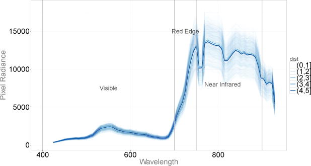
Spectral responses from 2,500 pixels corresponding to five different binned distances with superimposed fitted mean curves.

Although interest in point-wise inference is obvious, few viable approaches exist in this direction that account for inflated false positive results and correlation structure among tests. Ramsay and Silverman (2005) proposed a method for performing L point-wise tests simultaneously, however their approach is not designed to control the family-wise error rate (FWER) – i.e., the probability of at least one false rejection among all tests. A promising approach was introduced by Cox and Lee (2008) who used the multiplicity correction procedure proposed by Westfall and Young (1993) to control the FWER. Neither of the proposed methods provide a decision regarding the overall null hypothesis that all single L hypotheses are true. This is an undesirable property since a multiple comparison procedure may be non-coherent (Gabriel (1969)), i.e., the rejection of at least one point-wise hypothesis may not imply the rejection of the overall null and thus might lead to interpretation problems.

We propose a point-wise procedure that both provides a decision for the overall hypothesis and adequately adjusts the individual p-values to account for L simultaneous tests. The method first uses two different p-value combining methods to summarize the associated evidence across L points, defines a new test statistic, W, based on the smallest p-value from the two combination methods, and applies the closure principle of Marcus et al. (1976) to individually adjust the L point-wise p-values. The idea of using the minimum p-value as the test statistic for the overall test across different combination methods has been used in genetics studies (Hoh et al. (2001), Chen et al. (2006), Yu et al. (2009)). A challenge for the proposed analysis was the individual adjustment performed using the closure principle. The closure principle generally requires 2^L − 1 tests. To overcome this obstacle, we describe a computational shortcut which allows individual adjustments using the closure method even for large L. Accordingly, the paper is organized as follows. We give an overview of the closure principle and detail the computational shortcut to it. We give an explicit strategy for the proposed approach and compare its performance to other possibilities in a simulation study. We apply the proposed methodology in order to identify regions of the electromagnetic spectrum that differ based on distances to a simulated underground CO₂ leak pipe.

2 Multiple Tests and Closure Principle

2.1 The General Testing Principle

It is well known that by construction all inferential methods have a nonzero probability of Type I error. Therefore, when L multiple tests are conducted simultaneously, the probability of finding at least one spurious result is greater than the threshold α. A multiple testing adjustment procedure, which controls FWER for the family of individual hypotheses, H₁,…, H_L, at a pre-specified level α, can be obtained through the closure principle of Marcus et al. (1976). The closure principle considers all possible combination hypotheses obtained via the intersection of the set of L individual hypotheses H_I = ∩{H_i : i ∈ I}, I ⊆ {1,…, L}. The coherence of the procedure is enforced by rejecting an individual hypothesis H_i, i = 1,…, L, only if all intersection hypotheses that contain it as a component are rejected. Most researchers prefer the results of a multiple test procedure to be presented in terms of L individually adjusted p-values. The individually adjusted p-value for the hypothesis H_i is set to the maximum p-value of all intersection hypotheses implied by H_i.

A valuable feature of the closure principle is its generality, i.e., any suitable α-level test can be used to test the intersection hypotheses. However, the implementation of the method becomes computationally challenging for a large number of tests. The total number of intersection hypotheses is 2^L − 1 which grows quickly with L and limits the applicability of the method. Grechanovsky and Hochberg (1999) exhaustively discussed the conditions under which the closure procedure admits a shortcut in the case of joint multivariate normal tests. The question remains of how to reduce the computational burden of the closure method in the case of non-normal correlated tests.

2.2 Closure in a Permutation Context

Permutation-based methods are becoming more popular for multiple testing corrections with high-dimensional data. They do not require normality assumptions and utilize the data-based correlation structure. That is, the resulting procedure for false positive decision corrections based on permutation test is exact despite unknown covariance structure. The closure method easily admits permutation-based tests, all that is required is an α-level permutation test for each intersection hypothesis. Westfall and Troendle (2008) described a computational shortcut for the closure principle with a permutation test that reduces the number of required computations from the order of 2^L to L. Here, we show how to implement a computational shortcut for the Šidák (Šidák (1967)) and Fisher (Fisher (1932)) permutation-based tests to reduce the number of computations from the order of 2^L to the order of L².

Suppose K tests are conducted and the resulting p-values are p₁,…,p_K. Denote the ordered p-values by p₍₁₎ ≤ ⋯ ≤ p_(K). The test based on the Šidák correction for the intersection of K hypothesis, ${\cap }_{i=1}^K{H}_i$, is

$$S_K=1-{(1-p_{(1)})}^K.$$ (1)

The Fisher test statistic for the same intersection hypothesis is

$$F_K=-2{\displaystyle \sum _{i=1}^K\text{ln}{p}_i.}$$ (2)

The permutation p-values based on the Šidák correction are equivalent to the p-values based on the min-p test statistic and the rank truncated product statistic (RTP), $W\left(K\right)={\displaystyle {\prod }_{i=1}^K{p}_{\left(i\right)}}$, of Dudbridge and Koeleman (2003) with truncation at K = 1, because 1 − (1 − p₍₁₎)^K is a monotonic transformation of p₍₁₎. Similarly, $-2{\displaystyle {\sum }_{i=1}^K\text{ln}{p}_i}$ is a monotonic transformation of ${\displaystyle {\prod }_{i=1}^K{p}_{\left(i\right)}}$, and the permutation p-values based on these two test statistics are equivalent.

The idea behind the shortcut is to consider only the “worst” (the smallest) test statistic in the subsets of the same cardinality. Note that, for both the Šidák correction-based test and the Fisher test, the values of the test statistics are monotonically decreasing among intersection hypotheses of the same size. Thus, for the ordered p-values, p₍₁₎ ≤ ⋯ ≤ p_(L), the hypotheses that will be used for individual adjustments are:

$$\begin{array}{ll}\text{for}{H}_1,\hfill & \left\{H_1\text{,}{H}_{1L},H_{1L(L-1)},\dots ,H_{1L\dots 2}\right\};\hfill \\ \text{for}{H}_2,\hfill & \left\{H_2\text{,}{H}_{2L},H_{2L(L-1)},\dots ,H_{2L\dots 1}\right\};\hfill \\ \text{for}{H}_3,\hfill & \left\{H_3\text{,}{H}_{3L},H_{3L(L-1)},\dots ,H_{3L\dots 1}\right\};\hfill \\ ⋮\hfill & ⋮\hfill \\ \text{for}{H}_L,\hfill & \left\{H_L\text{,}{H}_{L(L-1)},H_{L(L-1)(L-2)},\dots ,H_{L(L-1)\dots 1}\right\}.\hfill \end{array}$$

Here, the hypothesis H₁ has p-value p₍₁₎, H₂ has p-value p₍₂₎, etc. The unique intersection hypotheses to consider are highlighted in bold, and the number of unique tests to consider is $1+2+\cdots L=\frac{L\left(L+1\right)}{2}$. One need not necessarily use resampling to apply the above shortcut, however it also works well if permutations are used to find p-values for each intersection hypothesis. Figure 1 illustrates correspondence between p-values calculated based on the full closure “resampling-based” procedure and the “resampling-based” shortcut. The graphs show an excellent agreement between the two adjusted p-values for both Šidák and Fisher test statistics.

Figure 1.

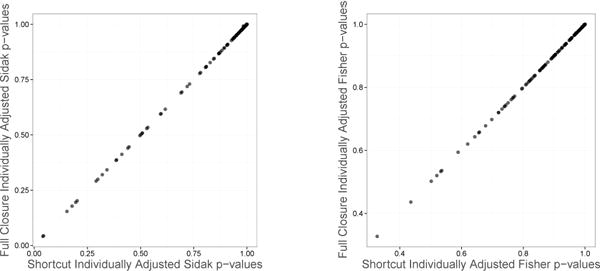
Correspondence between individually adjusted p-values using the full closure algorithm and the computational shortcut (L = 10). The Šidák p-values are illustrated in the left panel, and the Fisher p-values in the right panel.

3 Methods

We now describe a permutation algorithm that ensures coherency when estimating adjusted individual p-values. Suppose L correlated tests are conducted simultaneously. Apply the following steps to obtain the corresponding individually adjusted p-values based on B permutations.

1. Construct $\frac{L\left(L+1\right)}{2}\times \left(B+1\right)$ matrices of Šidák and Fisher permuted test statistics, S_ij, F_ij $i=1,\dots ,\frac{L\left(L+1\right)}{2}$ (indexes intersection hypotheses), j = 1, …, B + 1 (indexes permutations). The first column of the matrices contains the observed test statistics.

2. Construct $\frac{L\left(L+1\right)}{2}\times \left(B+1\right)$ matrices of the permuted p-values based on the algorithm from Ge et al. (2003) – discussed below. The Šidák p-value for the i-th intersection hypothesis and j-th permutation is

   $$P_{ij}^s=\frac{1}{B}{\displaystyle \sum _{k=1,k\ne j}^{B+1}I\left(S_{ik}\le S_{ij}\right).}$$

   The Fisher p-value for the i-th intersection hypothesis and j-th permutation is

   $$P_{ij}^f=\frac{1}{B}{\displaystyle \sum _{k=1,k\ne j}^{B+1}I\left(F_{ik}\ge F_{ij}\right).}$$
3. Define the statistic $W_{ij}=\text{min}\left(P_{ij}^S,P_{ij}^f\right)$ and obtain its p-value as

   $$P_i^W=\frac{1}{B}{\displaystyle \sum _{k=2}^{B+1}I\left(W_{ik}\le W_{i1}\right),}i=1,\dots ,\frac{L\left(L+1\right)}{2}.$$

4. Make an overall decision and obtain L individually adjusted p-values by applying the closure principle to the set of $P_i^W$’s.

To avoid nested permutations in Step 2, we used the algorithm by Ge et al. (2003) to compute permutational p-values for each permutation j = 2,…, B + 1. More specifically, the algorithm allows one to obtain permutational p-values on just B permutations instead of B². Also, in Step 3, testing the i^th intersection hypothesis with W_ij at a threshold α would lead to inflated Type I error rate, because choosing the smallest of the two p-values $P_{ij}^S$ and $P_{ij}^f$ leads to yet another multiple testing problem. To overcome this issue, one can use either the Bonferroni correction and define the test statistic as 2 min(P^s, P^f) or, as suggested, determine the significance of W on the basis of permutations. Finally, setting W=min(P^S, P^f) is the same as min(RTP(1), RTP(L)), where RTP(•) is the rank truncated product statistic of Dudbridge and Koeleman (2003) which was also considered in Zaykin (2000) and Zaykin et al. (2007). Thus, W incorporates two extremes: the combination of all p-values and a min-p adjustment procedure. Simulation studies are used to show that it retains desired properties of both type of statistics.

4 Simulations

4.1 Simulation Study Setup

We were motivated by a problem of identifying differences in mean spectral signatures of healthy vegetation and vegetation under stress across electromagnetic spectra. We approach the problem by evaluating functional responses on a grid of 80 points across wavelengths and performing tests point-wise. More generally, we were interested in evaluating k groups of functional responses on a grid of L points, t₁, …, t_L, and performing point-wise inference in the functional data setting. The goal of the simulation study was to investigate the power of the proposed procedure to detect departures from (1) the global null hypothesis ${\cap }_{i=1}^L{H}_i$ of no difference anywhere in t and (2) the point-wise null hypotheses H₀ : μ₁(t_i) = μ₂(t_i) for all t_i, i = 1, …, L, where μ(t_i) is a mean functional response evaluated at a point t_i. We followed the setup of Cox and Lee (2008) to be able to directly compare the performance of W to their method. To the best of our knowledge, the Cox and Lee (2008) method is the only viable existing approach for performing point-wise inference with functional data so we considered it to be a direct competitor.

For all simulations we generated two samples of functional data with n₁ = n₂ = 250 observations in each group (N = 500). The mean function of the first sample was constant and set to zero, μ₁(t) ≡ 0, t ∈ [0,1]. The mean of the second sample was either set to μ₂(t) = γBeta(1000,1000)(t) or μ₃(t) = γBeta(5,5)(t), where Beta is a probability density function of the Beta distribution. Figure 2 illustrates μ₂(t) and μ₃(t) for the range of different γ values explored.

Figure 2.

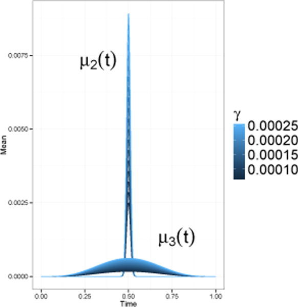
Two choices for the mean of the second sample.

First, we simulated the case where all L point-wise hypotheses were true (μ₁(t_i) ≡ μ₂(t_i), ∀t_i). To obtain functional data, we evaluated the mean functions on a grid of 140 equally spaced points ranging from −0.2 to 1.2 and added random noise, ε_ij ~ N (0,0.01²). Then, we fitted a smoothing spline using the <monospace>smooth.spline</monospace> R function (R Core Team (2013)) with the 0.95 smoothing parameter for each functional observation as suggested in Cox and Lee (2008). The output of the <monospace>smooth.spline</monospace> function is the fitted values of functional responses evaluated on the original grid of points. We disposed of 20 points from each end to remove excessive boundary variability from the estimated splines and for each curve sub-sampled 50 equally spaced values on the grid between 0 and 1. At the 0.05 level, we evaluated the empirical Type I error rate for the global null, i.e., the number of incorrect rejections of the overall null hypothesis, ${\cap }_{i=1}^{50}{H}_i$, out of B = 1000 simulations. We also evaluated the empirical control of the family-wise error rate (FWER), i.e., the number of times at least one incorrect rejection occurred across all points where the null hypothesis is true. We calculated the FWER control in a weak sense, meaning that H_i was true for all i = 1, …, 50, and in a strong sense, meaning that not all point-wise H_i’s were true. Reporting the empirical FWER was not a trivial task due to the computational intensity of the methods. Likely for this reason, Cox and Lee (2008) never reported the FWER in their original paper. To obtain our results, we employed the Boos and Zhang (2000) method that allowed us to reduce the size of the inner resampling loop and correct the resulting estimator for bias.

We also compared our procedure to five alternative statistical methods: the Šidák correction based test, the Fisher test, the Cox and Lee method (Cox and Lee (2008)), the functional ℱ statistic (Shen and Faraway (2004)), and the functional V_n (Cuevas et al. (2004)). The functional test statistics of Shen and Faraway (2004) and Cuevas et al. (2004) are designed to perform the overall functional analysis of variance (FANOVA) test. The FANOVA null and alternative hypotheses are

$$\begin{array}{ll}{H}_0:\hfill & {\mu }_1\left(t\right)={\mu }_2\left(t\right)=\dots ={\mu }_k\left(t\right)\hfill \\ H_a:\hfill & {\mu }_i\left(t\right)\ne {\mu }_{i\prime }\left(t\right),\text{for}\text{at}\text{least}\text{one}t\text{and}i\ne i\prime ,\hfill \end{array}$$

where μ_i(t) is assumed to be fixed, but unknown, population mean function of group i, i = 1, …, k. Parametric distributions are available for both ℱ and V_n from the original papers. The FANOVA test assesses evidence for the existence of differences among population mean curves across the entire functional domain. The test across the entire domain of t is a global test. Thus, we also considered these two methods as competitors to the proposed methodology.

Second, we investigated two properties of our method: (1) power to detect deviations from the combined null hypothesis ${\cap }_{i=1}^{50}{H}_i$ and (2) power to detect deviations from point-wise hypotheses H₁, H₂, …, H₅₀. To calculate power for the combined null hypotheses, we simulated B = 1000 sets of functional observations for the specified range of γ values, performed the overall test and calculated the empirical probability of rejecting ${\cap }_{i=1}^{50}{H}_i$. At the point-wise level, the concept of power is not as clear cut. For example, one may calculate conjunctive power – the probability of rejecting all false null hypotheses – or disjunctive – the probability of rejecting at least one false hypothesis. For a detailed discussion of these different choices see Bretz et al. (2010). Here, we adopted the approach of Cox and Lee (2008) to be able to directly compare to their results. We considered a single simulated set of functional observations for a specific choice of γ; calculated the unadjusted point-wise p-values; performed the multiplicity adjustment using W, as well as by Fisher’s, Šidák’s, and Cox & Lee’s methods; then we compared the adjusted p-values by plotting them on a single graph.

4.2 Results

Table 1 summarizes control of the Type I error rate for the overall null hypothesis, ${\cap }_{i=1}^{50}{H}_i$, the family-wise error rate (FWER) in the weak sense for the point-wise tests (all H_i’s are true) and the strong sense (only 28% of H_i’s are true at t₁₉, …, t₃₂). All methods tend to be liberal in terms of the Type I error rate control (“combined null” line). The family-wise error rate (both weak and strong control) is conservative for Šidák’s test, Fisher’s test and W, and right around 0.05 margin for the Westfall-Young adjustment.

Table 1.

The Type I error for the global null $\left({\cap }_{i=1}^L{H}_i\right)$ and the FWER for L = 50 tests, 1000 simulations, and α = 0.05.

	Šidák	Fisher	W	Cox & Lee	ℱ	Vn
combined null	0.059	0.065	0.060	NA	0.059	0.057
FWER weak	0.021	0.001	0.019	0.049	NA	NA
FWER strong	0.020	0.032	0.037	0.053	NA	NA

Figure 3 illustrates power for the global null hypothesis $\left({\cap }_{i=1}^L{H}_i\right)$. We see that in both graphs Fisher’s method outperforms all of the other methods, however W has similar power for this realization. The performance of the functional ℱ of Shen and Faraway (2004) is very similar to the functional V_n of Cuevas et al. (2004). The Šidák test is the clear laggard.

Figure 3.

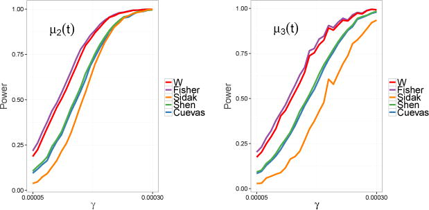
Plots of empirical power for the combined null hypothesis with α = 0.05.

Figure 4 shows the unadjusted and the adjusted p-values for a single set of functional observations. To compute the unadjusted p-values, we simulated 250 curves with mean μ₁(t) = 0 and μ₂(t) = 0.0003Beta(1000,1000)(t) (left graph) or μ₁(t) = 0 and μ₃ = 0.0003Beta(5, 5)(t) (right graph) and performed a t-test on a grid of 50 equally spaced points t₁ = 0, …, t₅₀ = 1. From both graphs, it is evident that Fisher’s method has the lowest power. The performance of W is very similar to Šidák’s test. The Cox & Lee method has the highest power.

Figure 4.

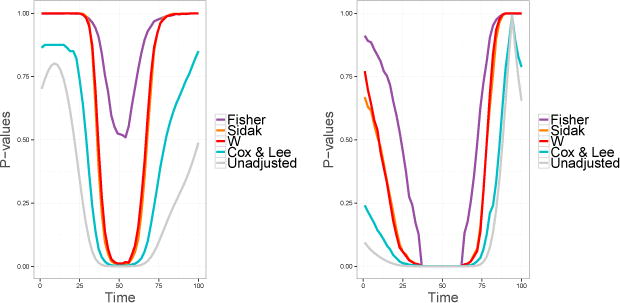
Plots of point-wise adjusted p-values for γ = 0.0003. Left graph: H_i : μ₁(t_i) = μ₂(t_i), i = 1, …, L. Right graph: H_i : μ₁(t_i) = μ₃(t_i), i = 1, …, L.

5 Application to Carbon Dioxide Data

Bellante et al. (2013) conducted an experiment to study the effect of carbon dioxide (CO₂) surface leak on vegetation stress at the Montana State University Zero Emission Research and Technology (ZERT) site in Bozeman, MT. To study the spectral changes in overlying vegetation in response to elevated soil CO₂ levels, a time series of aerial images was acquired over a buried carbon dioxide release pipe. A single image acquired on June 21, 2010 was the focus of the current analysis. The pixel-level measurements (with nearly 32,000 pixels) of the image consist of 80 spectral responses ranging from 424 to 929 nm. For each pixel, a horizontal distance to the CO₂ release pipe was calculated and 500 spectral responses were randomly chosen from five distance subcategories: (0,1], (1,2], (2,3], (3,4], and (4,5] meters (see Figure 5). To obtain a functional response for each pixel, we used the penalized cubic B-spline smoother with a smoothing parameter determined by generalized cross-validation (Ramsay et al. (2012)). The functional responses were evaluated on the original grid of L = 80 points and subsequently the analysis of variance test was performed point-wise to obtain the unadjusted p-values.

First, we tested the global null hypothesis of no difference in the entire range of spectral responses based on the distance from the CO₂ release pipe and obtained the corresponding overall p-value of 0.001 (from 1,000 permutations) using W. We then obtained the corrected point-wise p-values, which are illustrated in Figure 6. The adjusted p-values from 712 to 788 nm were below α = 0.05 and correspond to the “red edge” spectral region, which indicates that the spectral responses among binned distances differ significantly within this region. This is an encouraging result since previous research has indicated that the “red edge” spectral region is typically associated with plant stress (Carter and Knapp (2001)). Furthermore, the implementation of our method allows one to obtain an overall p-value over the points with established statistical significance. In our application, the points with the adjusted p-values below α = 0.05 were t₄₆, …, t₅₈, between 712 and 788 nm. Using the closure principle, we were also able to calculate the adjusted p-value=0.001 for the hypothesis ${\cap }_{i=46}^{58}{H}_i$, of no difference of group means in this region of the spectral domain.

Figure 6.

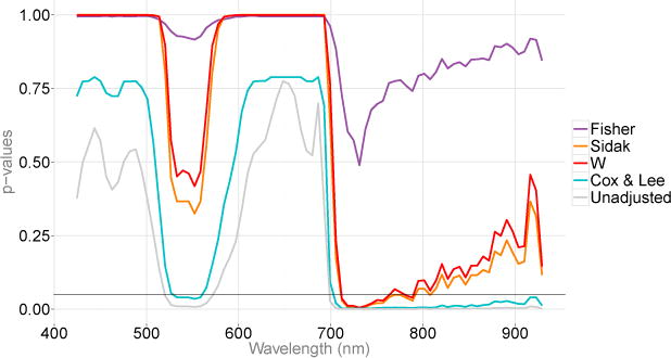
Plots of unadjusted and adjusted p-values. A horizontal line at 0.05 is added for a reference.

The method proposed by Cox and Lee (2008), which employs the Westfall-Young correction for multiplicity, identifies a much larger region of wavelengths than the other methods. The difference in power is due to the conservative nature of W. A possible direction of future research could be a correction to increase the FWER and the power of W.

6 Discussion

Modern data recording techniques allow one to sample responses at a high frequency of measurement. In many applications it is of interest to utilize all of the recorded information and perform a test at each point, while accounting for the correlation of the test statistics at nearby times, properly controlling the probability of false positive findings, and providing information on the overall difference. Here, we suggested a coherent method for point-wise testing with the desired properties.

Our method capitalizes on the evidence based on the minimum p-value (the Šidák method) and the product (or the sum on the logarithmic scale) of all p-values (the Fisher method). This results in a procedure that has high power for the combined null hypothesis, ${\cap }_{i=1}^L{H}_i$, and for the individual tests H₁, H₂, …, H_L. These characteristics of our procedure can be better understood by examining rejection regions of Fisher’s and Šidák’s tests. In general, rejection regions for L tests are hypervolumes in L-dimensional space, however some conclusions can be drawn from considering just two p-values. The two-dimensional rejection regions for Fisher’s and Šidák’s tests are provided in Loughin (2004). Based on the rejection regions, a clear difference is evident between the Fisher method and the Šidák method. In particular, the Fisher method will reject the combined null hypothesis, ${\cap }_{i=1}^L{H}_i$, if at least some p-values are “small enough”, but not necessarily significant. The Šidák method will reject the combined null hypothesis only if min-p is significant. Thus, Fisher’s method is higher-powered than Šidák’s method for the overall null hypothesis. On the other hand, Fisher’s test along with the closure principle is lower-powered than Šidák’s method for the individual adjustments. Envision a situation where the smallest p-value, p₍₁₎, is just above α. The adjusted value of p₍₁₎ by the closure principle is the maximum p-value of all hypotheses implied by H₍₁₎. To test an intersection hypothesis of size K, Fisher’s test considers the combination of p₍₁₎,p_(L), …, p_(L−K+1). All p_(L), …, p_(L−K+1) are greater than p₍₁₎ and Fisher’s test will not be able to reject ${\cap }_{i=1}^K{H}_i$ and thus H₍₁₎. Conversely, the decision for ${\cap }_{i=1}^K{H}_i$ based on Šidák’s test is made regardless of the magnitudes of p_(L), …, p_(L−K+1) but solely on the magnitude of p₍₁₎. Thus, Šidák’s method along with the closure principle has higher power than Fisher’s method for the individual tests H₁, H₂, …, H_L. Since our approach combines Fisher and Šidák’s methods, it possesses desirable properties of both tests and has high power for all ${\cap }_{i=1}^L{H}_i$ and H₁, H₂, …, H_L.

Our method uses the closure principle of Marcus et al. (1976) to adjust the point-wise p-values for multiplicity. The implementation of the closure method provides an additional advantage of being able to obtain a corrected p-value for intersection hypotheses of interest. That is, once the points with the adjusted p-values below a significance level α are identified, a researcher can obtain an overall p-value over the collection of these points. For example, in our application the points corresponding to the “red edge” spectral region (t₄₆, …,t₅₈) had statistically significant adjusted p-values. By using the closure principle we were additionally able to obtain a p-value for the intersection hypothesis ${\cap }_{i=46}^{58}{H}_i$ for the entire “red edge” interval. Thus, while the Westfall-Young approach appears to have higher power for testing individual hypotheses, overall p-values for subsets of the functional domain are not available with that approach.

Our method is permutation-based. Generally, a drawback of the permutations methods is their computational intensity. However, Cohen and Sackrowitz (2012) note that parametric stepwise multiple testing procedures (including the closure principle) are not designed to account for a correlation structure among hypotheses being tested. That is, test statistics for an intersection hypothesis will always be the same regardless of the correlation structure among tests considered. Thus, the shortcoming of the stepwise procedures is determining a correct critical value. The permutation-based approach alleviates this shortcoming and allows for dependency to be incorporated into the calculation of the critical values.

Another advantageous property of our method is that it does not require access to the original data but only to the L unadjusted point-wise p-values. The matrices of the test statistics in Step 1 can be found based on the Monte Carlo algorithm described in Zaykin et al. (2002). The test statistics are found by first obtaining L × 1 vectors, R^*, of independent random values from the Unif (0,1) distribution and then transforming them to R – vectors with components that have the same correlation structure as the observed p-values. Since functional observations are evaluated on a dense grid of points, the correlation structure among observed p-values can be estimated with reasonable precision. Thus, our method efficiently employs information contained just in the p-values and is more flexible than methods that require access to the original observations.

In summary, we proposed a coherent p-value combination method that allows researchers to obtain individually adjusted p-values for multiple simultaneous correlated tests. We hope that our work will promote new research in this direction. In particular, in our approach we treated all p-values as equally important. It might be possible to incorporate some weights that would optimize desirable properties of the procedure based on a particular application. Alternatively, adaptive selection of the test statistic is possible. That is, instead of considering just min-p (RTP(1)) and the combination of all p-values (RTP(L)), one might optimize power and size of the proposed method by considering RTP(K) across all possible values of K = 1, …,L.

References

- Bellante J, Powell S, Lawrence R, Repasky K, Dougher T. Aerial detection of a simulated co2 leak from a geologic sequestration site using hyperspectral imagery. International Journal of Greenhouse Gas Control 2013 [Google Scholar]
- Boos DD, Zhang J. Monte carlo evaluation of resampling-based hypothesis tests. Journal of the American Statistical Association. 2000;95:486–492. [Google Scholar]
- Bretz F, Hothorn T, Westfall P. Multiple Comparisons Using R. Chapman & Hall/CRC; 2010. [Google Scholar]
- Carter G, Knapp A. Leaf optical properties in higher plants: linking spectral characteristics to stress and chlorophyll concentration. American Journal of Botany. 2001;88:677–684. [PubMed] [Google Scholar]
- Chen B, Sakoda L, Hsing A, Rosenberg P. Resamplingbased multiple hypothesis testing procedures for genetic casecontrol association studies. Genetic Epidemiology. 2006;30:495–507. doi: 10.1002/gepi.20162. [DOI] [PubMed] [Google Scholar]
- Cheverud J. A simple correction for multiple comparisons in interval mapping genome scans. Heredity. 2001;87:52–58. doi: 10.1046/j.1365-2540.2001.00901.x. [DOI] [PubMed] [Google Scholar]
- Cohen A, Sackrowitz H. The interval property in multiple testing of pairwise- differences. Statistical Science. 2012;27(2):294–307. [Google Scholar]
- Cox DD, Lee JS. Pointwise testing with functional data using the westfall-young randomization method. Biometrika. 2008;95(3):621–634. [Google Scholar]
- Cribbie RA. Multiplicity control in structural equation modeling. Structural Equation Modeling. 2007;14(1):98–112. [Google Scholar]
- Cuevas A, Febrero M, Fraiman R. An anova test for functional data. Computational Statistics & Data Analysis. 2004;47:111–122. [Google Scholar]
- Dudbridge F, Koeleman B. Rank truncated product of p-values, with application to genomewide association scans. Genetic Epidemiology. 2003;25:360–366. doi: 10.1002/gepi.10264. [DOI] [PubMed] [Google Scholar]
- Fisher R. Statistical methods for research workers. Oliver and Boyd; London: 1932. [Google Scholar]
- Gabriel KR. Simultaneous test procedures – some theory of multiple comparison. Annals of Mathematical Statistics. 1969;40:224–250. [Google Scholar]
- Ge Y, Dudoit S, Speed T. Resampling-based multiple testing for microarray data analysis. Test. 2003;12:1–44. [Google Scholar]
- Godwin A, Takaharab G, Agnewc M, Stevensond J. Functional data analysis as a means of evaluating kinematic and kinetic waveforms. Theoretical Issues in Ergonomics Science. 2010;11(6):489–503. [Google Scholar]
- Grechanovsky E, Hochberg Y. Closed procedures are better and often admit a shortcut. Journal of Statistical Planning and Inference. 1999;76:79–91. [Google Scholar]
- Hoh J, Wille A, Ott J. Trimming, weighting, and grouping snps in human case-control association studies. Genome Research. 2001;11:2115–2119. doi: 10.1101/gr.204001. [DOI] [PMC free article] [PubMed] [Google Scholar]
- Li J, Ji L. Adjusting multiple testing in multilocus analysis using the eigenvalues of a correlation matrix. Heredity. 2005;95:221–227. doi: 10.1038/sj.hdy.6800717. [DOI] [PubMed] [Google Scholar]
- Loughin T. A systematic comparison of methods for combining p-values from independent tests. Computational Statistics & Data Analysis. 2004;47:467–485. [Google Scholar]
- Marcus R, Peritz E, Gabriel KR. On closed testing procedures with special reference to ordered analysis of variance. Biometrika. 1976;63(3):655–660. [Google Scholar]
- Nyholt D. A simple correction for multiple testing for single-nucleotide polymorphisms in linkage disequilibrium with each other. American Journal of Human Genetics. 2004;74:765–769. doi: 10.1086/383251. [DOI] [PMC free article] [PubMed] [Google Scholar]
- R Core Team. R: A Language and Environment for Statistical Computing. R Foundation for Statistical Computing; Vienna, Austria: 2013. URL http://www.R-project.org. [Google Scholar]
- Ramsay JO, Silverman BW. Functional Data Analysis. 2nd. Springer; 2005. [Google Scholar]
- Ramsay JO, Wickham H, Graves S, Hooker G. fda: Functional Data Analysis. R package version 2.3.2. 2012 URL http://CRAN.R-project.org/package=fda.
- Rice W. Analyzing tables of statistical tests. Evolution. 1988;43(1):223–225. doi: 10.1111/j.1558-5646.1989.tb04220.x. [DOI] [PubMed] [Google Scholar]
- Shen Q, Faraway J. An f test for linear models with functional responses. Statistica Sinica. 2004;14:1239–1257. [Google Scholar]
- Šidák Z. Rectangular confidence regions for the means of multivariate normal distributions. Journal of the American Statistical Association. 1967;78:626–633. [Google Scholar]
- Westfall P, Troendle J. Multiple testing with minimal assumptions. Biometrical Journal. 2008;50:745–755. doi: 10.1002/bimj.200710456. [DOI] [PMC free article] [PubMed] [Google Scholar]
- Westfall P, Young S. Resampling-based Multiple Testing: Examples and Methods for p-Values Adjustment. Wiley; 1993. [Google Scholar]
- Yu K, Li Q, Bergen A, Pfeiffer R, Rosenberg P, Caporasi N, Kraft P, Chatterjee N. Pathway analysis by adaptive combination of p-values. Genetic Epidemiology. 2009;33:700–709. doi: 10.1002/gepi.20422. [DOI] [PMC free article] [PubMed] [Google Scholar]
- Zaykin DV. Ph.D thesis. North Carolina State University; 2000. Statistical analysis of genetic associations. [Google Scholar]
- Zaykin DV, Zhivotovsky LA, Czika W, Shao S, Wolfinger RD. Combining p-values in large-scale genomics experiments. Pharm Stat. 2007;6(3):217–226. doi: 10.1002/pst.304. [DOI] [PMC free article] [PubMed] [Google Scholar]
- Zaykin DV, Zhivotovsky LA, Westfall PH, Weir BS. Truncated product method for combining p-values. Genetic Epidemiology. 2002;22(2):170–185. doi: 10.1002/gepi.0042. [DOI] [PubMed] [Google Scholar]