Multi-Output Decision Trees for Lesion Segmentation in Multiple Sclerosis

Abstract

Multiple Sclerosis (MS) is a disease of the central nervous system in which the protective myelin sheath of the neurons is damaged. MS leads to the formation of lesions, predominantly in the white matter of the brain and the spinal cord. The number and volume of lesions visible in magnetic resonance (MR) imaging (MRI) are important criteria for diagnosing and tracking the progression of MS. Locating and delineating lesions manually requires the tedious and expensive efforts of highly trained raters. In this paper, we propose an automated algorithm to segment lesions in MR images using multi-output decision trees. We evaluated our algorithm on the publicly available MICCAI 2008 MS Lesion Segmentation Challenge training dataset of 20 subjects, and showed improved results in comparison to state-of-the-art methods. We also evaluated our algorithm on an in-house dataset of 49 subjects with a true positive rate of 0.41 and a positive predictive value 0.36.

1. INTRODUCTION

Multiple Sclerosis (MS) is a chronic, demyelinating disease affecting the central nervous system. The demyelination leads to formation of lesions or sclera, primarily in the white matter (WM) in the brain and spine. These lesions are visible as hyperintensities in fluid attenuated inversion recovery (FLAIR) sequence images and as hypointensities in T₁-weighted (T₁-w) images (see Fig. 1). Depending on the type of MS, lesions can increase or decrease in number and volume as a function of time. Lesion count is one of the criteria for diagnosing MS,¹ and lesion volumes can be used to track disease progression.² Lesions are highly variable in their appearance, location, and volume in MRI. In addition, the FLAIR sequence also suffers from artifacts,³ which make lesion segmentation a challenging task. Accurate delineation requires aligning multimodal data and visualizing the tissue boundaries and is a difficult task, even for experienced manual raters. Delineating the lesion-WM boundary can be especially subjective and variable. Manual segmentation also suffers from large intra- and inter-rater variability.⁴ Thus, an automated, fast, and accurate lesion segmentation method is crucial in order to segment and analyze large patient imaging studies.

Figure 1.

The first row shows an algorithm result with a high TPR and PPV from the CHB dataset. The second row shows a low TPR and PPV result from the UNC dataset.

There has been significant work in the area of MS lesion segmentation.^5–14 Llado et al.¹⁵ in their survey analyze many recently published automated lesion segmentation techniques, both qualitatively and quantitatively. Some of the methods investigated in the survey were the best performing solutions as determined by the MICCAI 2008 MS Lesion Segmentation Challenge (MSLSC).¹⁶ The winning entry of the MSLSC estimated a threshold for FLAIR images based on the intensity distribution of the gray matter.⁵ Shiee et al.⁶ segmented MS lesions along with a topologically correct full brain segmentation. Recent work by Geremia et al.⁷ has surpassed the performance of the MSLSC winner.

2. NEW WORK TO BE PRESENTED

Our approach is similar to Geremia et al.,⁷ in that we also implement binary decision trees that are learned from intensity and context features. However, instead of predicting the label at a single voxel, as most methods do, we predict an entire neighborhood or patch for a given input feature vector. Lesion boundaries often seem to appear at slightly shifted locations in different modalities. Thus knowledge of predicted tissue classes in neighboring voxels is useful in determining the class of the central voxel. To achieve this, we have implemented a version of multi-output decision trees, which are similar in essence to the output kernel trees developed by Geurts et al.¹⁷ Predicting entire neighborhoods gives us further context information such as the presence of lesions predominantly inside white matter. We post-process the segmentations produced by our multi-output decision trees to reduce false positives.

3. METHOD

Co-registered T₁-w, FLAIR, and T₂-w images as well as expert manual segmentations are used as training data in our supervised learning approach. We denote this data collection as $\{{ℐ}_p^{(T_1)},{ℐ}_p^{(F)},{ℐ}_p^{(T_2)},{ℐ}_p^{(L)}\}$, p = 1, …, N for the images from the p^th training subject, corresponding to the T₁-w, FLAIR, T₂-w, and labeled image, respectively.

3.1 Preprocessing

All images undergo preprocessing including N4 bias correction,¹⁸ rigid registration to the 1 mm³ MNI space,¹⁹ skull stripping,²⁰ and finally intensity standardization. The T₁-w images are intensity standardized by linear scaling of the WM peak of the intensity histogram to match the intensity of a reference image. The FLAIR and T₂-w images are intensity standardized by fixing the histogram mode to a reference by a linear scaling.

3.2 Features

For the p^th training image set, ${ℐ}_p^{(T_1)}$, ${ℐ}_p^{(F)}$, ${ℐ}_p^{(T_2)}$, at each voxel i, we extract small u × v × w-sized patches. Let these patches be $x_i^{(T_1,p)}$, $x_i^{(F,p)}$, $x_i^{(T_2,p)}$, respectively for the input modalities. In our experiments we use u = v = w = 3. Small patches provide us with local context of a particular voxel. However due to the variability of lesion appearance and variations in the FLAIR images due to artifacts, just local intensity information cannot distinguish between lesion and normal tissue. Thus we augment the local patches with features that provide global context for a voxel.

For each voxel i, we locate a voxel j, which is at a distance of r from i in a radial direction from i. By radial direction we mean the unit vector in the direction of voxel i from the center of the MNI space. We calculate the mean intensity of a large window of size w₁ × w₂ × w₃ (11 × 11 × 3) about the voxel j. This radial patch average provides a good indication of location in the brain relative to the cortex. Let these window averages be $y_i^{(T_1,p)}$, $y_i^{(F,p)}$, $y_i^{(T_2,p)}$, respectively for each modality. The final feature vector is created by concatenating $\left[x_i^{(T_1,p)},x_i^{(F,p)},x_i^{(T_2,p)},y_i^{(T_1,p)},y_i^{(F,p)},y_i^{(T_2,p)}\right]=X_i$. The corresponding voxel i in the manually labeled training image ${ℐ}_p^{(L)}$ has a u × v × w-sized local patch surrounding it. We denote it by z_i. For a given training feature vector X_i, we have a corresponding dependent label vector z_i. The label vector is a binary vector as the classification is lesions vs normal tissue, but it can easily be used for a multi-class classification by assigning additional labels to the different tissues. [X_i; z_i] are sampled from all the training samples to create the training set.

3.3 Learning Multi-output Decision Trees

Learning a multi-output decision tree is similar to the CART algorithm²¹ to learn a single output regression tree. Let Θ_q = {[X₁; z₁], …, [X_m; z_m]} be the set of all the training sample pairs at a node q in the tree. The output vectors z_i are also known dependent vectors. Let dimensionality of the dependent vectors be d and the node mean at node q be ${\overline{z}}_q$. The squared distance (SD) from the mean for the dependent vectors at node q is,

$${\mathrm{SD}}_q={\displaystyle \sum _{k=1}^m{\displaystyle \sum _{j=1}^d{(z_{ij}-{\overline{z}}_{qj})}^2.}}$$ (1)

If a particular feature, f, and a threshold for the feature, τ_f are chosen, then the data in q, Θ_q is separated into two disjoint subsets, Θ_qL = {[X_i; z_i]|∀i, X_if ≤ τ_f} and Θ_qR = {[X_i; z_i]|∀i, X_if > τ_f}. f and τ_f are chosen such that the combined SD of the two daughter nodes q_L and q_R of q, is minimized.

The splitting is done recursively until there are a minimum number of samples left in a node, which is then declared as a leaf node of the tree. In our experiments, we have used fifty as the minimum number of leaf samples. Since a single tree is considered as a weak learner, we train multiple (five, in our experiments) trees using bootstrap aggregation (bagging) to create an improved classifier.

3.4 Prediction

Given a test image set consisting of processed T₁-w, T₂-w and FLAIR images, we extract the aforementioned features at each of the voxels. Next we apply the trained multi-output tree ensemble to each extracted feature vector. The input vector travels through the tree as its features are evaluated against the ones in the tree nodes, until it lands in a leaf node. The leaf node consists of at least fifty training samples, each of dimensionality d, with a label at each dimension. This provides us with 50d voxel labels, from which we determine the percentage of lesion voxels. This gives a membership estimate of a voxel belonging to the lesion class vs the normal tissue class.

3.5 Postprocessing

The membership image acquired from the multi-output decision ensemble is smoothed using a Gaussian filter with σ = 1. The smoothed membership image is thresholded to created a binary lesion mask. The threshold was empirically set to 0.33 to ensure a balance between true positive rate (TPR) and positive predictive value (PPV). Since a large majority of the MS lesions occurs inside white matter, we mask out false positives detected in other tissues. We use a simple three class fuzzy k-means segmentation²² of the T₁-w image to roughly identify a WM mask. Lesions, being hypointense in T₁-w images, appear as holes in this WM mask, which are filled.

4. RESULTS

4.1 MS Lesion Segmentation Challenge

For our first experiment we used the MSLSC Training Dataset.¹⁶ We compared the results with the winner of MSLSC⁵ and one of the current top ranked results,⁷ published after the challenge. We report some of the challenge metrics and compare the estimated lesion volume with the true lesion volume. MSLSC consists of twenty subjects, ten each from the University of North Carolina (UNC) center and the Children’s Hospital Boston (CHB), with T₁-w, FLAIR, T₂-w, and manual lesion segmentations. We randomly selected four subjects as training data and evaluated on the remainder. We also performed a leave-one-out classification of the four training data images to include them in the analysis.

Our algorithm performs generally better than the challenge winner.⁵ The results are in Table 1. In comparison to Geremia et al., our algorithm has a better TPR-PPV balance for the CHB data and performs worse for the UNC data. The large errors in the UNC data are of the type shown in the second row of Fig. 1, where the manual segmentation is debatable. Fig. 2(a) shows a scatter plot of the manual lesion volumes vs. those calculated by the algorithm. In an ideal scenario, the line fit on the scatter plot should match the identity line (black dashed line). Our algorithm slightly overestimates the lesion volume for the low lesion images, while underestimating for the high lesion volume images.

Table 1.

Average TPR and PPV values across 10 subjects for each of the UNC and CHB datasets, reported for 3 methods. We also evaluated our algorithm on an In-House dataset of 49 subjects.

	Souplet et al.5		Geremia et al.7		Our Algorithm
Dataset	TPR	PPV	TPR	PPV	TPR	PPV
CHB	0.138	0.364	0.350	0.552	0.400	0.400
UNC	0.257	0.236	0.447	0.255	0.361	0.194
In-House MS Dataset					0.407	0.358

Figure 2.

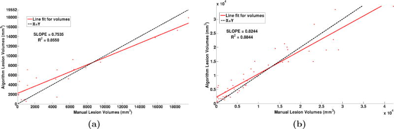
(a) Volume scatter plot and linear fit for the MSLSC data and (b) our in-house MS dataset.

4.2 In-house MS Data Segmentation

We also used an internal dataset of MS patients that was annotated by an expert rater. Our In-house MS data consists of MS patients consisted of forty nine subjects with T₁-w, P_D-w, T₂-w and FLAIR images. T₁-w images were acquired using the Magnetization Prepared Gradient Echo (MPRAGE) sequence and were acquired at a 0.82 × 0.82 × 1.1 mm³ resolution. Whereas the other scans were acquired at either 0.82 × 0.82 × 2.2 mm³ for 36 subjects and at 0.82 × 0.82 × 4.4 mm³ for 13 subjects. Thus this dataset has considerable internal variability.

All the images were preprocessed as before in the MNI space. We again used four random subjects as our training data. We have reported the average TPR and PPV value over all the subjects in Table 1 and the algorithm lesion volumes vs. manual lesion volumes in Fig 2(b). We can observe that our algorithm slightly overestimates the lesion volume for the low lesion load images, and underestimates for the high lesion load images. Results on two subjects with high and low lesion loads respectively are shown in Fig 3.

Figure 3.

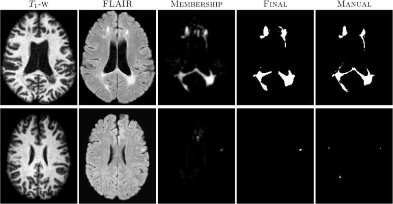
In-house MS dataset images with corresponding segmentation results. The top row shows results on a subject with a high lesion load, while the bottom row shows the results of subject with a low lesion load.

5. CONCLUSION AND FUTURE WORK

We have described a multi-output decision tree ensemble framework for MS lesion segmentation. Our approach produces results, which are comparable to the state-of-the-art. It is computationally very fast, taking about 1–2 minutes for a 181 × 217 × 181-sized image. We have evaluated our algorithm on the training dataset of the MS lesion segmentation challenge and also on our in-house collection of MS images. Currently the splitting criterion considers a squared distance from the mean for the dependent vectors z_i located at a node. However this criterion is not ideal as the z_i consist of discrete labels. We would like to improve our approach by considering a different metric, which is more akin to the Gini index developed for a typical single output decision tree for the purpose of classification. We would also like to explore more features in order to reduce the amount of false positives.

We have submitted the MS Challenge private test data for the MSLSC to the testing website and have not received the evaluation results by the time of submission of the final manuscript. These results will be made available on http://www.iacl.ece.jhu.edu/ when we receive them.

References

- 1.Polman CH, Reingold SC, Banwell B, Clanet M, Cohen JA, Filippi M, Fujihara K, Havrdova E, Hutchinson M, Kappos L, Lublin FD, Montalban X, O’Connor P, Sandberg-Wollheim M, Thompson AJ, Waubant E, Weinshenker B, Wolinsky JS. Diagnostic criteria for multiple sclerosis: 2010 Revisions to the McDonald criteria. Annals of Neurology. 2011;69(2):292–302. doi: 10.1002/ana.22366. [DOI] [PMC free article] [PubMed] [Google Scholar]
- 2.Rovira A, Swanton J, Tintor M. A single, early magnetic resonance imaging study in the diagnosis of multiple sclerosis. Archives of Neurology. 2009;66(5):587–592. doi: 10.1001/archneurol.2009.49. [DOI] [PubMed] [Google Scholar]
- 3.Stuckey S, Goh T-D, Heffernan T, Rowan D. Hyperintensity in the Subarachnoid Space on FLAIR MRI. American Journal of Roentgenology. 2007;189(4):913–921. doi: 10.2214/AJR.07.2424. [DOI] [PubMed] [Google Scholar]
- 4.Simon J, Li D, Traboulsee A, Coyle P, Arnold D, Barkhof F, Frank J, Grossman R, Paty D, Radue E, Wolinsky J. Standardized MR Imaging Protocol for Multiple Sclerosis: Consortium of MS Centers Consensus Guidelines. American Journal of Neuroradiology. 2006;27(2):455–461. [PMC free article] [PubMed] [Google Scholar]
- 5.Souplet J, Lebrun C, Ayache N, Malandain G. An Automatic Segmentation of T2-FLAIR Multiple Sclerosis Lesions. 2008 [Google Scholar]
- 6.Shiee N, Bazin PL, Ozturk A, Reich DS, Calabresi PA, Pham DL. A Topology-Preserving Approach to the Segmentation of Brain Images with Multiple Sclerosis Lesions. NeuroImage. 2010;49(2):1524–1535. doi: 10.1016/j.neuroimage.2009.09.005. [DOI] [PMC free article] [PubMed] [Google Scholar]
- 7.Geremia E, Clatz O, Menze BH, Konukoglu E, Criminisi A, Ayache N. Spatial decision forests for MS lesion segmentation in multi-channel magnetic resonance images. NeuroImage. 2011;57(2):378–390. doi: 10.1016/j.neuroimage.2011.03.080. [DOI] [PubMed] [Google Scholar]
- 8.Roy S, He Q, Carass A, Jog A, Cuzzocreo JL, Reich DS, Prince J, Pham D. Example based lesion segmentation. Proc SPIE. 2014;9034:90341Y–90341Y-8. doi: 10.1117/12.2043917. [DOI] [PMC free article] [PubMed] [Google Scholar]
- 9.Roy S, Carass A, Shiee N, Pham D, Prince J. Mr contrast synthesis for lesion segmentation. Biomedical Imaging: From Nano to Macro, 2010 IEEE International Symposium on. 2010 Apr;:932–935. doi: 10.1109/ISBI.2010.5490140. [DOI] [PMC free article] [PubMed] [Google Scholar]
- 10.Sweeney EM, Shinohara RT, Shiee N, Mateen FJ, Chudgar AA, Cuzzocreo JL, Calabresi PA, Pham DL, Reich DS, Crainiceanu CM. OASIS is Automated Statistical Inference for Segmentation, with applications to multiple sclerosis lesion segmentation in MRI. NeuroImage: Clinical. 2013;2(0):402–413. doi: 10.1016/j.nicl.2013.03.002. [DOI] [PMC free article] [PubMed] [Google Scholar]
- 11.Shiee N, Bazin PL, Cuzzocreo JL, Ye C, Kishore B, Carass A, Calabresi PA, Reich DS, Prince JL, Pham DL. Robust Reconstruction of the Human Brain Cortex in the Presence of the WM Lesions: Method and Validation. Human Brain Mapping. 2014;35(7):3385–3401. doi: 10.1002/hbm.22409. [DOI] [PMC free article] [PubMed] [Google Scholar]
- 12.Lecoeur J, Ferré J, Barillot C. Optimized Supervised Segmentation of MS Lesions from Multi-spectral MRIs. MICCAI workshop on Med Image Anal on Multiple Sclerosis. 2009:1–11. [Google Scholar]
- 13.Forbes F, Doyle S, García-Lorenzo D, Barillot C, Dojat M. Adaptive weighted fusion of multiple MR sequences for brain lesion segmentation. 7th International Symposium on Biomedical Imaging (ISBI 2010) 2010:69–72. [Google Scholar]
- 14.Van Leemput K, Maes F, Vandermeulen D, Colchester A, Suetens P. Automated segmentation of multiple sclerosis lesions by model outlier detection. Medical Imaging, IEEE Transactions on. 2001 Aug;20:677–688. doi: 10.1109/42.938237. [DOI] [PubMed] [Google Scholar]
- 15.Llado X, Oliver A, Cabezas M, Freixenet J, Vilanova JC, Quiles A, Valls L, Rami-Torrent L, Rovira lex. Segmentation of multiple sclerosis lesions in brain mri: A review of automated approaches. Information Sciences. 2012;186(1):164–185. [Google Scholar]
- 16.Styner M, Lee J, Chin B, Chin M, Commowick O, Tran H, Markovic-Plese S, Jewells V, Warfield S. 3D Segmentation in the Clinic: A Grand Challenge II: MS lesion segmentation. 2008 [Google Scholar]
- 17.Geurts P, Touleimat N, Dutreix M, d’Alche Buc F. Inferring biological networks with output kernel trees. Bioinformatics, BMC. 2007 May;8 doi: 10.1186/1471-2105-8-S2-S4. [DOI] [PMC free article] [PubMed] [Google Scholar]
- 18.Tustison N, Avants B, Cook P, Zheng Y, Egan A, Yushkevich P, Gee J. N4ITK: Improved N3 Bias Correction. IEEE Trans Med Imag. 2010 Jun;29:1310–1320. doi: 10.1109/TMI.2010.2046908. [DOI] [PMC free article] [PubMed] [Google Scholar]
- 19.Collins DL, Holmes CJ, Peters TM, Evans AC. Automatic 3-D model-based neuroanatomical segmentation. Human Brain Mapping. 1995;3(3):190–208. [Google Scholar]
- 20.Carass A, Cuzzocreo J, Wheeler MB, Bazin PL, Resnick SM, Prince JL. Simple Paradigm for Extra-cerebral Tissue Removal: Algorithm and Analysis. NeuroImage. 2011;56(4):1982–1992. doi: 10.1016/j.neuroimage.2011.03.045. [DOI] [PMC free article] [PubMed] [Google Scholar]
- 21.Breiman L, et al. Classification and Regression Trees. Wadsworth Publishing Company; U.S.A: 1984. [Google Scholar]
- 22.Bezdek JC. A Convergence Theorem for the Fuzzy ISO-DATA Clustering Algorithms. IEEE Trans on Pattern Anal Machine Intell. 1980;20(1):1–8. doi: 10.1109/tpami.1980.4766964. [DOI] [PubMed] [Google Scholar]