Harmonizing Diffusion MRI Data Across Multiple Sites and Scanners

Abstract

Harmonizing diffusion MRI (dMRI) images across multiple sites is imperative for joint analysis of the data to significantly increase the sample size and statistical power of neuroimaging studies. In this work, we develop a method to harmonize diffusion MRI data across multiple sites and scanners that incorporates two main novelties: i) we take into account the spatial variability of the signal (for different sites) in different parts of the brain as opposed to existing methods, which consider one linear statistical covariate for the entire brain; ii) our method is model-free, in that no a-priori model of diffusion (e.g., tensor, compartmental models, etc.) is assumed and the signal itself is corrected for scanner related differences. We use spherical harmonic basis functions to represent the signal and compute several rotation invariant features, which are used to estimate a regionally specific linear mapping between signal from different sites (and scanners). We validate our method on diffusion data acquired from four different sites (including two GE and two Siemens scanners) on a group of healthy subjects. Diffusion measures such fractional anisotropy, mean diffusivity and generalized fractional anisotropy are compared across multiple sites before and after the mapping. Our experimental results demonstrate that, for identical acquisition protocol across sites, scanner-specific differences can be accurately removed using the proposed method.

1 Introduction

Multi-site diffusion imaging studies are increasingly being used to study several disorders such, Alzheimer’s disease, Huntington’s disease, schizophrenia etc. However, intra-site variability in the acquired data sets poses a potential problem for joint analysis of diffusion MRI data [1,2]. Thus, aggregating data sets from different sites is challenging due to the inherent differences in the acquired images from different scanners. Although the inter-site variability of neuroanatomical measurements can be minimized by acquiring images using similar type of scanners (same vendor and version) with similar pulse sequence parameters and same field strength [3], many recent studies have shown that there still exist large differences between diffusion measurements from different sites [4]. This inter-site variability in the measurements can come from several sources, e.g., subject physiological motion, number of head coils used for measurement (16 or 32 channel head coil), imaging gradient non-linearity as well as scanner related factors [5]. This can cause non-linear changes in the images acquired as well as the estimated diffusion measures such as fractional anisotropy (FA) and mean diffusivity (MD). Inter-site variability in FA can be upto 5% in major white matter tracts and between 10-15% in gray matter areas [1]. On the other hand, FA differences in diseases such as schizophrenia are often of the order of 5%. Thus, harmonizing data across sites is imperative for joint analysis of the data.

Broadly, there are two approaches used to combine data sets from multiple sites. One approach is to perform the analysis at each site separately, followed by a meta-analysis as in [6]. Another standard practice is to use a statistical covariate to account for signal changes that are scanner-specific [7]. The first approach (meta-analysis) does not allow for a “true” joint analysis of the data, while the second method requires the use of a statistical covariate for each diffusion measure analyzed. Further, the latter method is inadequate to analyze results from tractography where tracts travel between distant regions. For example, in the cortico-spinal tract, scanner related differences in the brain stem might be quite different from those in the cortical motor region. Thus, using a single statistical covariate for the entire tract may produce false positive or false negative results. Consequently, region-specific scanner differences should be taken into account for such type of analyses. Another alternative is to add a statistical covariate at each voxel in a voxel based analysis method, however, such methods are susceptible to registration errors.

2 Our Contributions

In this work, we propose a novel scheme to harmonize diffusion MRI data from multiple scanners, taking into account the brain region-specific difference in the acquired signal from different scanners. Our method harmonizes the acquired signal at each site compared to a reference site using several rotation invariant spherical harmonic (RISH) features. A region specific linear mapping is proposed between the rotation invariant features to remove scanner specific differences in the white matter between a group of age-matched subjects at each site. The method uses model-free SH features¹ and thus is independent of any modeling assumptions, making it useful to be used for any type of future analysis (e.g., using single or multi-compartment models). To the best of our knowledge, this is a first work that has explicitly addressed the issue of dMRI data harmonization without the use of statistical covariates. Since the mapping is obtained from a set of healthy controls, it will not alter the signal due to disease or pathology, while ensuring that we do not directly modify model-based diffusion features such as FA, which are used in population studies [6].

3 Method

Figure 1 shows an outline of the proposed dMRI data harmonization method. Our goal is to map the dMRI data from a target site to an arbitrarily chosen reference site. We start by computing a set of rotation invariant spherical harmonic (RISH) features from the estimated SH coefficients. A region-specific linear mapping between the RISH features is then computed to map the dMRI data from target site to the reference site. Next, a secondary mapping is computed that appropriately updates each of the SH coefficients at each voxel in the brain. From the mapped SH coefficients, the mapped diffusion signal is computed at the desired set of gradient directions for each subject in the target site.

Fig. 1.

Outline of the proposed method for inter-site dMRI data harmonization

3.1 Diffusion MRI and RISH Features

Let S = [s₁…s_G]^T represent the dMRI signal along G unique gradient directions. In the spherical harmonic (SH) basis, the signal S can be written as [8]: S ≈ Σ_i Σ_j C_ij Y_ij, where Y_ij is a SH basis function of order i and phase j and C_ij are the corresponding SH coefficients. It is well-known that the “energy” or ${\mathbb{L}}_2$ norm of the SH coefficients for each order forms a set of rotation invariant (RISH) features [9]:

$${\parallel C_i\parallel }^2=\sum _{j=1}^{2i+1}{\left(C_{\mathit{ij}}\right)}^2.$$ (1)

One can think of the RISH features ∥C_i∥² as being the total energy at a particular frequency (order) in the SH space. Given the RISH features for N_k subjects for the k^th site (the target site), we compute the expected value as the sample mean:

$${\mathbb{E}}_k\left(\right[{\parallel C_i\parallel }^2\left]\right)=\sum _{n=1}^{N_k}\left[{\parallel C_i\left(n\right)\parallel }^2\right]∕N_k.$$ (2)

In this work, we computed the RISH features for order {0, 2, 4, 6} and ignored the higher order terms as they are the high frequency terms primarily capturing noise in the data. However, if required, the proposed methodology is quite general and can be extended to SH of any order.

3.2 Mapping RISH Features Between Sites

Figure 2 shows the RISH features of different orders computed for each site as well as for different anatomical regions of the brain. In particular, we used Freesurfer [10] software to parcellate the brain into different regions and subsequently grouped them into the following anatomical regions for each hemisphere: frontal, parietal, temporal, occipital, brain stem, cerebellum, the cingulate-corpus-callosum complex and centrumsemiovale-insula. For each of these white matter regions and for each site, we computed the sample average ${\mathbb{E}}_k$(·) (Eq. 2) of the RISH features shown in Figure 2. Clearly, these features vary significantly between sites as well as for different regions, showing that a regionally specific mapping is required to ensure proper harmonization of the diffusion data.

Fig. 2.

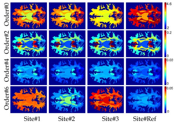
RISH features in the white matter for different SH orders and sites.

Given two groups of subjects that are matched for age, gender, handedness and socio-economic status, we expect that at a group level, they will have similar diffusion profiles and hence none of the RISH features should be statistically different between any two sites (or scanners). In other words, the diffusion measures between two groups of matched subjects (healthy) are statistically different only due to scanner differences. Thus, our aim is to find a proper mapping Π(·) for the RISH features such that all scanner related group differences between two sites are removed, i.e.,

$${\mathbb{E}}_k\left(\Pi \right({\parallel C_i\parallel }^2\left)\right)={\mathbb{E}}_r\left({\parallel C_i\parallel }^2\right),$$ (3)

where r is the reference site and k is the target site. Any difference in the sample mean for the two sites (or scanners) k and r can be computed as the difference $\Delta \mathbb{E}={\mathbb{E}}_r-{\mathbb{E}}_k$. By linearity of the expectation operator, the mapping for each subject n is given by:

$$\Pi \left({\parallel C_i\left(n\right)\parallel }^2\right)={\parallel C_i\left(n\right)\parallel }^2+{\mathbb{E}}_r-{\mathbb{E}}_k.$$ (4)

Note that, this mapping Π(·) only gives the amount of shift required to remove any scanner specific “group” differences. Thus, this mapping is only at the population level and a separate mapping is required that will change the individual SH coefficient at each voxel such that equation Eq. 4 is satisfied. We should also note that the mapping Π(·) is different for different RISH features even for the same ROI. For a subject n, we have the following map:

$$\Pi \left({\parallel C_i\left(n\right)\parallel }^2\right)=\sum _{j=1}^{2i+1}\pi \left(C_{\mathit{ij}}\right(n{)}^2)={\parallel C_i\left(n\right)\parallel }^2+\Delta \mathbb{E}=\sum _{j=1}^{2i+1}{C}_{\mathit{ij}}(n{)}^2+\Delta \mathbb{E}.$$ (5)

We extend this mapping to each voxel in an ROI, by uniformly changing the SH coefficients at each voxel v (we do not include the voxel indexing in our equations to keep the notation simple). There are two possible ways to obtain a mapping π(·) for each SH coefficient C_ij. One possibility is to use π(C_ij) = C_ij + δ (for all j) such that Eq. 5 is satisfied. However, this would entail adding a positive or negative constant δ to all coefficients (i.e. shifting the coefficients), which could potentially lead to a change in sign for coefficients that are smaller than δ. The effect of such a “shifting” operation is shown in Figure 3 (b), where the sign of some of the coefficients was changed by adding a small constant δ. This leads to a change in orientation and shape of the signal, which is erroneous and undesirable.

Fig. 3.

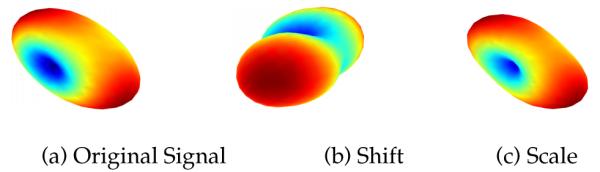
Effect of using different mapping functions π - shift vs scale. (a) Original dMRI signal. (b) π used as a shift map, (c) Estimated signal with π as a scaling map (Eq. 6).

A better mapping π(·) is to uniformly scale all the SH coefficients (belonging to a given SH order) so that Eq. 5 is satisfied. Such a mapping is given by:

$$\pi \left(C_{\mathit{ij}}\right)=\ell C_{\mathit{ij}},\text{where:}\ell =\sqrt{\frac{\Pi \left({\parallel C_i\left(n\right)\parallel }^2\right)}{{\parallel C_i\left(n\right)\parallel }^2}}.$$ (6)

Such scaling only changes the “size” of the signal and not its orientation, as seen in Figure 3 and as shown via experiments in the results section. The harmonized diffusion signal at each voxel v of a given ROI (for each subject n) is then computed using the mapped coefficients using $\widehat{S}(v,n)={\Sigma }_i{\Sigma }_j\pi \left(C_{\mathit{ij}}\right(v,n\left)\right){{\rm Y}}_{\mathit{ij}}$. Such a unique mapping is computed for each ROI and each subject in the target site.

4 Results

We used our method on data set acquired from 4 different sites and scanners; see Table 1 for details about each scanner as well as the number of subjects from each site. Nearly identical dMRI scan protocol was used at each site with the following acquisition parameters: spatial resolution of 2 × 2 × 2mm³, maximum b-value of b = 900s/mm² and TE/TR = 87/10000 ms. For the GE sites, the data was acquired with a 5/8 partial Fourier encoding, while the Siemens used 6/8 partial Fourier acquisition. Subjects at each site were age-matched to the group at the reference site.

Table 1.

Scanner details and subject numbers for each site.

Site#	Manufacturer	Field strength	Model	Software version	# of channels	# of subjects	# of directions
1	GE	3T	MR750	20×M4	8	10	86
2	GE	3T	MR750	M4	8	6	86
3	Siemens	3T	Tim Trio (102×32)	vb17	12	14	87
Ref.	Siemens	3T	Tim Trio (102×18)	VB15	12	10	87

An appropriate mapping was computed for each of the ROIs (obtained from Freesurfer) in each hemisphere of the brain as defined earlier. We tested our method by computing the p-value for the RISH features as well as standard diffusion measures. For each ROI, we computed if the RISH features were statistically different between the reference site and each of the target sites (site #1, #2, #3) and then used the algorithm described above to obtain the mapped signal. Due to space limitations, we have not provided the p-values for the RISH features in this paper, but all statistical differences were removed after the mapping. We also extensively tested our method on diffusion features that were not explicitly used in the mapping procedure, such as MD, FA, GFA and tensor orientation.

Table 2 gives the p-values for each of the ROIs (nomenclature – lFrontal is left-frontal and rFrontal is right-frontal lobe) before and after the harmonization of the data. Notice that MD was statistically different for almost all regions and sites as compared to the reference site, but these differences were completely removed. The p-value after mapping is almost 1 in this case following Eq. 6 and the fact that MD is directly proportional to the ${\mathbb{L}}_2$ norm of the SH coefficients. All statistical group differences between FA and GFA are also removed for each of the sites.

Table 2.

P-values before and after mapping for MD, FA, GFA for different sites and ROIs.

	MD						FA						GFA
	Site#1		Site#2		Site#3		Site#1		Site#2		Site#3		Site#1		Site#2		Site#3
	Before	After	Before	After	Before	After	Before	After	Before	After	Before	After	Before	After	Before	After	Before	After
lFrontal	2.4e-06	1	1.7e-08	1	1.6e-07	1	0.45	0.54	2.8e-02	0.43	0.21	0.93	6.0e-16	0.4	6.9e-03	0.62	2.6e-08	0.49
lParietal	6.5e-08	1	2.5e-07	1	1.1e-07	1	1.0e-04	0.25	7.8e-04	0.27	1.5e-03	0.41	1.5e-08	0.77	6.3e-02	0.53	1.1e-09	0.66
lTemporal	5.4e-09	1	3.3e-08	1	5.4e-08	1	0.18	0.47	3.9e-02	0.95	6.4e-02	0.71	3.8e-09	0.75	5.6e-02	0.84	4.2e-08	0.73
lOccipital	7.1e-06	1	2.2e-02	1	8.7e-07	1	6.4e-02	0.81	2.7e-02	0.76	3.3e-02	0.81	2.8e-08	0.93	0.82	0.85	1.6e-06	0.97
lCentrumSemi.	1.5e-10	1	8.9e-08	1	2.0e-08	1	4.7e-03	0.62	1.3e-05	0.90	1.3e-02	0.93	2.2e-12	0.93	0.42	0.7	7.8e-09	0.74
lCerebellum	5.6e-07	1	8.6e-05	1	1.7e-07	1	0.79	0.34	0.77	0.72	3.3e-02	0.73	7.5e-09	0.86	6.4e-02	0.86	1.1e-07	0.92
rFrontal	4.8e-06	1	1.7e-08	1	5.8e-10	1	0.19	0.61	8.6e-02	0.39	0.13	0.18	4.0e-09	0.89	1.4e-03	0.71	1.0e-09	0.23
rParietal	1.6e-06	1	2.1e-06	1	1.8e-07	1	2.8e-02	0.51	1.4e-03	0.84	7.7e-02	0.54	1.8e-07	0.91	0.2	0.94	4.5e-09	0.62
rTemporal	1.4e-06	1	7.4e-05	1	1.6e-06	1	0.55	0.39	9.6e-03	0.77	0.63	0.65	4.4e-08	0.86	7.5e-02	0.96	5.9e-08	0.62
rOccipital	5.5e-05	1	1.3e-02	1	3.0e-02	1	9.6e-02	0.91	1.2e-02	0.83	0.38	0.81	5.0e-07	0.89	7.4e-02	0.75	4.2e-09	0.71
rCentrumSemi.	8.7e-13	1	7.0e-09	1	3.7e-10	1	8.5e-04	0.98	8.8e-04	0.83	2.2e-03	0.78	6.4e-10	0.68	0.25	0.61	5.5e-06	0.50
rCerebellum	1.3e-06	1	4.9e-04	1	0.11	1	0.27	0.59	0.79	0.87	8.5e-04	0.95	5.1e-08	0.98	0.10	0.91	1.8e-08	0.90
BrainStem	5.6e-10	1	7.4e-06	1	1.2e-05	1	2.4e-04	0.67	7.6e-04	0.99	0.49	0.80	2.2e-06	0.65	0.22	0.88	4.0e-08	0.64

We also ran a TBSS study [11] for the FA values for each of the sites. Figure 4 shows widespread group differences between the subjects from the reference site (Siemens scanner) and site #1 (GE scanner). After data harmonization, most white matter group differences were removed confirming the results seen in Table 2. However, group differences in the sub-cortical regions are still seen, as that region was not “harmonized” or mapped for scanner differences. Extending the current methodology to gray matter and sub-cortical region is part of our future work.

Fig. 4.

TBSS results for site #1 before (a) and after (b) applying our method. The yellow-red colormap displays p-values less than 0.05. Only white matter regions were used in this work, and sub-cortical gray matter regions were not harmonized resulting in a statistical group difference in that region in (b).

We also compared the average error in degrees in the orientation of the fibers (estimated using the single tensor model and SH-based orientation distribution function (ODF)) at each voxel, before and after the mapping. For the tensor based model, the average change in orientation at each voxel was always less that 1^° resulting in the following average whole brain change in orientation for each site 0.7606 ± 0.1250^°, 0.1400 ± 0.0830^° and 0.7259 ± 0.2180^°, respectively. Change in orientations estimated from the discretized ODF’s were 0.24e-5^°, 0.17e-5^° and 0.26e-5^°, respectively for each site. We also computed the coefficient of variation (CV) in FA [1] for each site before and after the harmonization procedure (CV, before: 0.0321 ± 0.0121, 0.0285 ± 0.0137, 0.0579 ±0.0097 and after 0.0315 ± 0.0114, 0.0272 ± 0.0142, 0.0595 ± 0.0128 respectively). Thus within site CV did not change much after the mapping.

5 Conclusion and Limitations

In this work, we proposed a novel method that allows to harmonize the dMRI signal from different sites in a region-specific, subject-dependent manner, while maintaining the inter-subject variability at each site but removing scanner specific differences in the signal. Once such a mapping is computed from healthy subjects, it can then be used to map another cohort of diseased subjects without altering the signal due to disease or pathology. The proposed method is model independent and directly maps the signal to the reference site. The method can be of great use to aggregate data from multiple sites and making it feasible to do joint analysis of a large sample of data. We should note that, to the best of our knowledge, this is a first work that has explicitly addressed the issue of dMRI data harmonization without the use of statistical covariates.

Nevertheless, the proposed method has some limitations that we note: 1). It is dependent on the accuracy of Freesurfer segmentations, 2). It is possible that the ROIs used in this work are too large to remove local scanner-specific differences. One way to address this concern is to test if any sub-region within an ROI is still statistically different between two sites and subsequently obtain a separate mapping for such “smaller ROIs”. In this work, we did not harmonize gray matter and sub-cortical structures, however, the proposed method is general enough to be applied to these areas of the brain as well. Our future work will involve ways to address all these limitations. Further, the proposed method can be used to separately harmonize each b-value shell for multi-shell diffusion data.

References

- 1.Vollmar C, Muircheartaigh J, Barker G, Symms M, Thompson P, Kumari V, Duncan J, Richardson M, Koepp M. Identical, but not the same: Intra-site and inter-site reproducibility of fractional anisotropy measures on two 3.0 T scanners. NeuroImage. 2010:1384–1394. doi: 10.1016/j.neuroimage.2010.03.046. [DOI] [PMC free article] [PubMed] [Google Scholar]
- 2.Matsui J. Phd Thesis. University of IowaFollow; 2014. Development of image processing tools and procedures for analyzing multi-site longitudinal diffusion-weighted imaging studies. [Google Scholar]
- 3.Cannon T, McEwen FSS, Abd G, He XP, Erp T, Jacobson A, Beardon C, Walker E. Reliability of neuroanatomical measurements in a multi-site longitudinal study of youth at risk for psychosis. Human Brain Mapping. 2014;35:2424–2434. doi: 10.1002/hbm.22338. (in press) [DOI] [PMC free article] [PubMed] [Google Scholar]
- 4.Foxa R, Sakaieb K, Leec J, Debbinse J, Liuf Y, Arnoldg D, Melhem E, Smithh C, Philipsb M, Loweb M, Fisherd E. A validation study of multicenter diffusion tensor imaging: Reliability of fractional anisotropy and diffusivity values. AJNR Am. J. Neuroradiol. 2012;33:695–700. doi: 10.3174/ajnr.A2844. [DOI] [PMC free article] [PubMed] [Google Scholar]
- 5.Zhu T, Hu R, Qiu X, Taylor M, Tso Y, Yiannoutsos C, Navia B, Mori S, Ekholm S, Schifitto G, Zhong J. Quantification of accuracy and precision of multi-center dti measurements: a diffusion phantom and human brain study. Neuroimage. 2011;56:1398–1411. doi: 10.1016/j.neuroimage.2011.02.010. [DOI] [PMC free article] [PubMed] [Google Scholar]
- 6.Salimi-Khorshidi G, Smith S, Keltner J, Wager T, Nichols T. Meta-analysis of neuroimaging data: a comparison of image-based and coordinate-based pooling of studies. Neuroimage. 2009;25:810–823. doi: 10.1016/j.neuroimage.2008.12.039. [DOI] [PubMed] [Google Scholar]
- 7.Forsyth J, Cannon T, et al. Reliability of functional magnetic resonance imaging activation during working memory in a multi-site study: analysis from the north american prodrome longitudinal study. Neuroimage. 2014;97:41–52. doi: 10.1016/j.neuroimage.2014.04.027. [DOI] [PMC free article] [PubMed] [Google Scholar]
- 8.Descoteaux M, Angelino E, Fitzgibbons S, Deriche R. Regularized, fast, and robust analytical q-ball imaging. MRM. 2007;58:497–510. doi: 10.1002/mrm.21277. [DOI] [PubMed] [Google Scholar]
- 9.Kazhdan M, Funkhouser T, Rusinkiewicz S. Rotation invariant spherical harmonic representation of 3D shape descriptors. Symposium on Geometry Processing; 2003. [Google Scholar]
- 10.Fischl B, Liu A, Dale A. Automated manifold surgery: Constructing geometrically accurate and topologically correct models of the human cerebral cortex. IEEE TMI. 2001;20:70–80. doi: 10.1109/42.906426. [DOI] [PubMed] [Google Scholar]
- 11.Smitha S, Jenkinsona M, Johansen-Berga H, Rueckertb D, Nicholsc T, Mackaya C, Watkinsa K, Ciccarellid O, Cadera Z, Matthewsa P, Behrensa T. Tract-based spatial statistics: Voxelwise analysis of multi-subject diffusion data. NeuroImage. 2006;31:1487–1505. doi: 10.1016/j.neuroimage.2006.02.024. [DOI] [PubMed] [Google Scholar]