RTCR: a pipeline for complete and accurate recovery of T cell repertoires from high throughput sequencing data

Abstract

Motivation: High Throughput Sequencing (HTS) has enabled researchers to probe the human T cell receptor (TCR) repertoire, which consists of many rare sequences. Distinguishing between true but rare TCR sequences and variants generated by polymerase chain reaction (PCR) and sequencing errors remains a formidable challenge. The conventional approach to handle errors is to remove low quality reads, and/or rare TCR sequences. Such filtering discards a large number of true and often rare TCR sequences. However, accurate identification and quantification of rare TCR sequences is essential for repertoire diversity estimation.

Results: We devised a pipeline, called Recover TCR (RTCR), that accurately recovers TCR sequences, including rare TCR sequences, from HTS data (including barcoded data) even at low coverage. RTCR employs a data-driven statistical model to rectify PCR and sequencing errors in an adaptive manner. Using simulations, we demonstrate that RTCR can easily adapt to the error profiles of different types of sequencers and exhibits consistently high recall and high precision even at low coverages where other pipelines perform poorly. Using published real data, we show that RTCR accurately resolves sequencing errors and outperforms all other pipelines.

Availability and Implementation: The RTCR pipeline is implemented in Python (v2.7) and C and is freely available at http://uubram.github.io/RTCR/along with documentation and examples of typical usage.

Contact: b.gerritsen@uu.nl

1 Introduction

T cells are crucial to the adaptive immune system, enabling it to recognize almost any pathogen that infects the host while remaining tolerant to many self-antigens. The recognition of antigens by T cells is mediated by the T cell receptor (TCR). Through random genetic recombination, the immune system can potentially equip every T cell with a different TCR, allowing it to bind different antigens than other T cells. The different T cells together form a T cell repertoire, which due to its pivotal role in the immune response, is studied extensively in areas such as infectious diseases, cancer, autoimmunity and ageing (Bolotin et al., 2012; Suessmuth et al., 2015 ; Woodsworth et al., 2013).

Classical TCRs are heterodimers, consisting of αβ protein chains. The genes encoding the α and β chains are generated via somatic stochastic DNA rearrangements, in which germline variable (V), diversity (D) and joining (J) gene segments recombine (Bassing et al., 2002). Random deletions and non-templated nucleotide insertions occur at the V(D)J junctions, which together with the random selection of gene segments is responsible for generating a full repertoire of TCRs. Theoretically, ∼$5\times {10}^{11}$ different TCR β chains are possible (Robins et al., 2010), which together with the TCRα chains can result in more than 10¹⁵ distinct TCRs (Davis and Bjorkman, 1988). Because humans have ∼10¹² T cells (Arstila et al., 1999), every individual harbors at most only a small but diverse (Arstila et al., 1999; Robins et al., 2010; Qi et al., 2014; Warren et al., 2011) fraction of this potential repertoire.

High throughput sequencing (HTS) (Holt and Jones, 2008; Shendure and Ji, 2008) is often used to probe the TCR repertoire (Freeman et al., 2009; Klarenbeek et al., 2010; Ndifon et al., 2012; Robins et al., 2009, 2010; Wang et al., 2010; Warren et al., 2011). Analysing the repertoire is challenging because of its high diversity and many rare clonotypes, pushing the boundaries of sequencing technologies. Some of the important confounding factors in quantification and identification of the repertoire are: short read length (e.g. 150 bp reads whereas the VDJ region of the TCR is ∼500 bp), unequal polymerase chain reaction (PCR) amplification, sequencing errors and sampling biases (Baum et al., 2012; Calis and Rosenberg, 2014; Nguyen et al., 2011; Robins et al., 2009; Warren et al., 2011). Despite the improvements in sequencing technologies, quantification of true TCR repertoire diversity remains elusive, because the repertoire is heavily undersampled and sequencing errors artificially skew the repertoire.

To analyse HTS data from TCR repertoires, multiple pipelines have been developed. Some of these are: IMGT (Alamyar et al., 2012), which provides a web interface and detailed annotations, iSSAKE (Warren et al., 2009), which assembles immune receptors from very short reads, IRmap (Wang et al., 2010), designed for 454 sequencing data, Decombinator (Thomas et al., 2013), designed for fast annotation, MiTCR (Bolotin et al., 2013), MiXCR (Bolotin et al., 2015) and IMSEQ (Kuchenbecker et al., 2015) focusing on error correction, Presto (Vander Heiden et al., 2014) and MiGEC (Shugay et al., 2014) handling reads with unique molecular identifiers (‘barcoded’ data) and TCRklass (Yang et al., 2015) annotating all reads including those that lack the complementarity determining region 3 (CDR3) of the TCR. Most of these pipelines filter out low quality reads and/or remove rare TCR sequences. Since most unique TCR sequences are rare, such filtering can cause a massive loss of true TCR sequences.

We developed a pipeline, called Recover TCR (RTCR), that attempts to accurately recover TCR sequences at varying coverage, including rare TCR sequences while maintaining high precision and high recall. Accurate quantification of TCR repertoires is especially important in clinical settings, where low coverage TCR sequencing can be used for cost effectiveness. There are multiple ways to identify sequence errors in HTS data. Some of these are: (i) base quality, i.e. a low quality base is more likely to be false than a high quality base, and (ii) similarity, i.e. true TCR sequences tend to be surrounded by similar erroneous variants due to PCR and sequencing errors. In RTCR, these strategies are translated into a simple binomial model (Nguyen et al., 2011) together with several heuristics to rationally eliminate PCR and sequencing errors. RTCR automatically sets its parameters based on the data, relieving the user from setting arbitrary parameters. RTCR supports ‘barcoded’ HTS data, combining barcode-based error correction with its regular error correction.

To measure the performance of RTCR, we compared it to TCRklass, MiTCR, MiXCR, IMSEQ and MiGEC, using simulated and real HTS datasets. We demonstrate that RTCR can easily adapt to error profiles of different types of sequencers and exhibits consistently high recall and high precision even at low coverage. We benchmark different pipelines using several synthetic TCR HTS datasets generated via realistic PCR and sequencing simulations. We find that RTCR outperforms all other pipelines on recall and matches the high precision of MiTCR, MiXCR and IMSEQ. Using real data we then show that RTCR can accurately resolve apparent sequencing errors which are incompletely resolved by other pipelines.

2 Methods

2.1 RTCR pipeline

RTCR is a pipeline for identification and data-driven error correction of TCR sequences from HTS data. The pipeline was written in Python v2.7 and C, and provides an easy to use command line interface. Below we will explain the steps the RTCR pipeline takes to analyse an HTS dataset.

Reads obtained from HTS are typically too short to span the whole TCR gene and are error-prone. If a read contains the CDR3 region of a TCR, the corresponding TCR gene can be uniquely identified (provided the read also contains enough of the flanking V and J segment nucleotides to unambiguously determine the correct V and J segment). Every base in a read is assigned a ‘Phred’ score (Q), which indicates the probability (p) of an erroneous base call by the sequencer: $Q=-10{\log }_{10}p$. To infer TCR sequences, RTCR aligns germline V and J segments to the reads using an external aligner. We chose Bowtie 2 (Langmead and Salzberg, 2012) as the default aligner for RTCR, because it is fast, accurate (data not shown), and uses Phred scores to score the alignments. The pipeline can easily be configured to use a different aligner. The D segments are not aligned to the reads because it is difficult to align them unambiguously and excluding the D segments does not change the inference of a TCR sequence. RTCR uses the alignments to identify and extract the CDR3 region from every read, annotating it with the V and J segment identified by the aligner. Sets of identical CDR3 sequences are collapsed as follows: (i) a single CDR3 sequence is kept and assigned the number of sequences in the set as its abundance, (ii) each position in the CDR3 sequence is assigned the highest Phred score found at that position in the set and (iii) the CDR3 sequence is assigned the VJ segment combination most common in the set, breaking ties using the alignment score assigned by the aligner. An option is provided to the user to prevent RTCR from collapsing CDR3 sequences with identical CDR3 but different V and J segment annotation. We chose to collapse all identical CDR3 sequences by default to avoid generation of false TCR sequences due to ambiguity in segment annotation.

It is known that PCR and sequencing experiments can generate errors in some reads which would inflate the number of distinct TCR sequences (Baum et al., 2012; Bolotin et al., 2012; Nguyen et al., 2011). RTCR uses a simple statistical model to estimate the number of erroneous sequences in the data and the total number of errors these sequences may contain. Let ϵ be the probability of an error for a base in a read. If we assume all bases are independent and are erroneous with the same probability (ϵ), then a sequence (i.e. a string of bases) can be modeled as a set of Bernoulli trials. The probability of having exactly h errors in a sequence of length l is then given by the conventional binomial:

$$p_h=\left(\begin{array}{c}l\\ h\end{array}\right){\mathrm{ϵ}}^h{(1-\mathrm{ϵ})}^{l-h},\text{\hspace{0.5em}for\hspace{0.5em}\hspace{0.5em}}h\in \{0,1,\dots ,l\}.$$ (1)

Next, consider a set of n sequences, each of length l. There are $n\times p_h$ sequences expected to have exactly h errors, and the maximum number of errors expected to occur in at least one sequence is:

$$H=\max (\{h:n{p}_h\ge 1\}).$$ (2)

Consider for example n as the number of times a particular TCR sequence of length l has been sequenced, then there are expected to be np₀ correct copies of it in the data. The remaining $n(1-p_0)$ erroneous copies are spread across an unknown number of distinct variants and there is expected to be at least one erroneous copy having H mismatches with the TCR sequence.

The quality merge (QMerge), iterative merge (IMerge) and Levenshtein merge (LMerge) algorithms that are explained below, use Equations (1) and (2) together with several heuristics to determine which and how many sequences are likely to be erroneous. The algorithms depend primarily on the per base error rate (ϵ). RTCR estimates this error rate (ϵ) from the number of mismatches observed in the aligned germline sequences with the reads. RTCR calculates two separate error rates, one from the V alignments with the CDR3 region and one from the J alignments with the CDR3 region. To remain conservative in the number of distinct TCR sequences recovered, the higher of the two error rates is assigned to ϵ.

Both QMerge and IMerge group TCR sequences by length and error correct each length group independently. Due to stochasticity and experimental bias, the true number of mismatches in a length group may be higher or lower than expected given the error rate, ϵ, which was calculated using all TCR sequences in the HTS dataset. To prevent underestimation of the true number of mismatches in a length group, RTCR combines the information from the alignments and the base quality (Phred) scores to calculate a length group specific error rate (ϵ_l):

$${\mathrm{ϵ}}_l=\frac{m_a+m_u}{n},$$ (3)

where l is the length of the TCR sequences, n is the number of bases in the length group, m_a is the number of mismatches found in the aligned regions of the TCR sequences in the length group, and m_u is the number of mismatches expected in the unaligned regions of the TCR sequences, estimated using the base quality scores:

$$m_u={\displaystyle \sum _Q{u}_Q{10}^{\frac{-Q}{10\alpha }}},$$ (4)

where Q is a Phred score, u_Q, is the number of bases in the unaligned regions of the length group with a Phred score of Q, and α is a normalization factor for the Phred scores. Since Phred scores reflect the probability that a base is false, every Phred score can be recalculated by taking all aligned bases with a particular Phred score and use the fraction f that was false, to calculate an effective Phred score $Q_{\text{eff}}=-10{\log }_{10}f$. The normalization factor α is calculated from the average ratio of observed Phred scores to the effective Phred scores, $\alpha =\sum _{Q}Q/Q_{\text{eff}}$. Finally, RTCR takes the maximum of the globally calculated error rate (ϵ) and the group specific error rate (ϵ_l), $\max (\mathrm{ϵ},{\mathrm{ϵ}}_l)$, as the error rate for the length group in the QMerge and IMerge algorithms.

The error correction algorithms of RTCR described below (including barcode error correction) use the same approach to merging TCR sequences. If two (parent) TCR sequences are merged, a (child) consensus sequence is formed from the highest abundant base at every position, breaking ties by selecting the higher quality base, using ‘N’ if ties cannot be broken. The algorithms keep track of the frequencies of the parent bases at every position using a position frequency matrix (PFM). TCR(/consensus) sequences are merged by summing their associated PFMs and generating a consensus sequence from the resulting PFM. Hence, the final error corrected TCR sequence is independent of the order in which its parent TCR sequences were merged. Additionally, the error correction algorithms use the PFMs to keep track of the number of mutations that have been performed, by summing the frequencies of the bases that were not selected for the TCR sequences associated with the PFMs.

2.1.1 QMerge algorithm

QMerge groups sequences by length and merges sequences within each group based upon their abundance and base quality scores. Let n be the total number of sequences of length l under consideration. To prevent RTCR from merging unrelated sequences, QMerge uses Equation (2) and considers all pairs of sequences of length l differing by at most H bases. We define a ‘merge quality score’ as the sum of the minimum quality scores of all mismatching bases between two sequences:

$$m={\displaystyle \sum _{i\in \text{mismatches}}\min (q_i,q_i^{\prime })},$$ (5)

where q and $q^{\prime }$ are vectors, each containing the base quality scores of one of the two sequences in the pair; and mismatches contains the indices of the mismatching bases. QMerge uses the merge quality score to order the pairs and merge the lowest quality sequences first. We define a ‘quality threshold’:

$$Q=10{\log }_{10}nl,$$ (6)

which is the Phred score equivalent to the probability that one in n × l bases is false. QMerge calculates the merge quality score (m) for every pair of sequences (within Hamming distance (HD) H) and considers pairs for which $m\le Q$.

QMerge traverses sequence pairs in the following order: increasing merge quality score (m), HD and decreasing abundance of the more frequent sequence in the pair. A merge is not performed if it requires mutation of a base with a quality score higher than the median Phred score in the data. The child inherits the VJ annotation of the more abundant parent. Its abundance is the sum of the abundances of both parents. After a successful merge, the parent sequences are removed from the data. If the child matches an existing sequence, the child is merged to it. The merge quality score (m) is (re)calculated for all pairs of sequences involving the child. The algorithm halts when there are no more pairs to process or the expected number of false bases ($n\times l\times \mathrm{ϵ}$) in the set have been corrected.

2.1.2 IMerge algorithm

After performing QMerge many errors are expected to remain in the data. IMerge attempts to resolve these errors by using a clustering approach where less abundant sequences are merged to more abundant nearby sequences (Fig. 1). Like QMerge, IMerge also groups sequences by length and considers each group separately. Because true TCR sequences (green circles in Fig. 1) may differ by a single nucleotide substitution, their neighborhoods of erroneous sequences may overlap. IMerge resolves clusters gradually to prevent true TCR sequences from merging to each other. All TCR sequences of length l, starting with the most abundant, are allowed to absorb neighboring erroneous sequences (red circles in Fig. 1), starting with the rarest, within HD h in their neighborhood. The algorithm begins at h = 1 and increases h by one after every iteration over all sequences until there are no more sequences that can be merged.

Fig. 1.

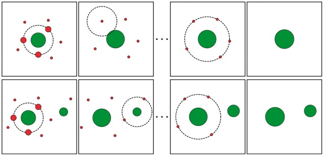
Schematic of IMerge algorithm. Top row shows one true TCR sequence (green) surrounded by erroneous variants (red); the diameter of symbols represents the abundance of the TCR sequence. IMerge considers all nearby TCR sequences as potential erroneous variants. Erroneous variants present at HD 1 can get merged to the true TCR sequence depending upon the abundance of the true sequence, abundance of erroneous variant and the error rate determined from the data (top row second column). Once all sequences at HD 1 are considered IMerge iterates over the TCR sequences considering all variants present at HD$\le$2. The bottom row demonstrates a scenario where two true TCR sequences are neighbors but do not get merged due to abundance and HD thresholds defined by Equations (2) and (8)

When IMerge considers a particular TCR sequence of length l, it estimates the true abundance of the TCR sequence. To not underestimate the true abundance of the TCR, IMerge calculates the 99% lower confidence interval using a normal approximation:

$$n=\frac{n_{\text{orig}}+z\sqrt{n_{\text{orig}}(1-p_0)}}{p_0},$$ (7)

where z is the 99% normal quantile, p₀ is the probability of having zero errors in a sequence (defined by Equation (1)), and $n_{\text{orig}}$ is the abundance of the TCR sequence in the original data ($n_{\text{orig}}=0$ for novel TCR sequences generated by QMerge). IMerge considers all neighboring sequences within HD H + 1 (where H is defined by Equation (2)) from the TCR sequence. IMerge calculates the expected abundance of a TCR sequence if this TCR sequence would absorb all its erroneous copies within HD h:

$$N_h=n_{\text{QMerge}}+\frac{n-n_{\text{QMerge}}}{1-p_0}{\displaystyle \sum _{d=1}^h{p}_d},$$ (8)

where $n_{\text{QMerge}}$ is the abundance of a TCR sequence obtained after QMerge; and $1\le h\le H+1$. IMerge orders all sequences (neighbors) within HD h by increasing abundance and minimum base quality score, and merges the neighbors to the TCR sequence. A merge is not performed if the resulting abundance of the TCR sequence would exceed N_h, i.e. its expected abundance if it would absorb all its erroneous copies until HD h (note, $N_H\approx n$). This limiting of the number of neighbors that can be absorbed within HD h allows true TCR sequences to protect themselves from being absorbed by merging their (erroneous) neighbors (Fig. 1). The algorithm halts when no merges can be performed for any TCR sequence.

2.1.3 LMerge algorithm

After the QMerge and IMerge algorithms, indels are expected to remain in the data (sometimes in combination with mismatches). RTCR estimates the expected number of deletions (insertions), n_d (n_i), from the number of deletions (insertions) found in the alignments of germline V and J sequences with the CDR3 region. The LMerge algorithm is similar to IMerge, with an important difference being that it calculates the Levenshtein instead of HD between TCR sequences. Similar to the IMerge stopping criteria, the LMerge algorithm also does not introduce more than n_d deletions or n_i insertions.

RTCR performs a post-processing step where CDR3 sequences with unresolved bases (‘N’) are merged to the nearest CDR3 sequence that differs with it only on the unresolved positions. Finally, CDR3 sequences containing a base quality score below five are discarded. This culling of low quality sequences is performed only after error correction.

2.2 Simulation of TCR HTS

We used the probabilistic model of Murugan et al. (2012) to simulate the biological process of rearranging V, D and J segments, generating a synthetic repertoire of 10⁴ TCRB chain sequences. Because TCRB sequences are generally too long to be spanned by reads, HTS protocols such as $5\prime$ RACE (Warren et al., 2011) are used to amplify the part of the TCRB sequence containing the CDR3 region. To get sequence lengths similar to the $5\prime$ RACE protocol we included only the first 61 bp of the constant region in the synthetic TCR sequences. To mimick the heavy-tailed distribution of TCRB sequences in humans (Mora et al., 2010; Venturi et al., 2011), we expanded the synthetic repertoire to 10⁵ sequences according an empirical TCRB distribution. This distribution was derived from lane SRR060714 of Warren et al. (2011) using MiTCR (Bolotin et al., 2013).

HTS protocols involve PCR amplification. PCR can distort sequence abundances (Best et al., 2014) because not all sequences are doubled in a PCR cycle and polymerases can have a sequence bias. Additionally, false but abundant TCR sequences can be formed if mutations occur in early PCR cycles. We simulated a simplified PCR process to introduce imperfect amplification and to generate TCR variants. In every cycle of in silico PCR the number of TCR sequences was doubled using sampling with replacement so that some sequences were missed in every doubling. Every TCR sequence was doubled ∼18 times, with a substitution error rate of $5\times {10}^{-5}$ (Cline et al., 1996), resulting in ${10}^5\times 2^{18}$ synthetic amplicons with ∼2% of the amplicons containing one or more PCR errors.

We used the Illumina simulator of ART (Huang et al., 2012) version 2.3.7 to generate paired-end reads from subsets of the synthetic amplicons. The size of the subset determined the fold coverage (i.e. number of reads per ‘cell’). For example, a subset of 10⁶ amplicons represents 10× coverage, because the synthetic repertoire consisted of 10⁵ TCRB sequences (and 10⁴ clonotypes), and ART generates at least one paired-end read for every amplicon in the subset. We simulated two recent sequencers, HiSeq 2500 and MiSeq, using the default error profiles provided by ART. For HiSeq (MiSeq) the settings were: read length 150 (250), mean fragment length 200 (500), standard deviation 15 (0). Finally, we merged read pairs as follows: read pairs with <18 bp paired end overlap were dropped; for overlapping regions a consensus sequence was created by selecting the higher quality base when bases agreed, or if one had $\ge$Q30 and the other <Q20, in all other cases an ‘N’ with Q0 was recorded.

2.3 Analysis of TCR HTS

Analyses were performed using TCRklass 0.6.0, MiTCR 1.0.3, MiXCR 1.6, IMSEQ 1.0.1, MiGEC 1.2.3 and RTCR 0.3.0, using the default settings. As ’default settings’ for IMSEQ we turned on its clustering based error correction and merging of identical CDR3 sequences with ambiguous segment identification, i.e. ‘-ma -qc -sc’. Before evaluating the performance of each pipeline, non-functional TCR sequences (i.e. those that are out-of-frame or contain a stop-codon) were removed. For the analyses of non-barcoded HTS data (real and simulated), all pipelines, with the exception of MiXCR which uses its own reference, were run with the germline reference sequences of MiTCR. For the analysis of barcoded HTS data, RTCR was run with the V(D)J reference sequences of MiGEC. To compare the error correction of MiGEC and RTCR, the latter was run on the sequences resulting from the Checkout utility of MiGEC so that both had the same starting point. MiGEC was run with an ‘overseq’ threshold of 5 (i.e. discarding UMI groups with fewer than five reads).

Both TCRklass and IMSEQ pipelines report identical CDR3 sequences with different VJ combinations by default which can inflate the false positive rate. To make the reporting equivalent among the pipelines, we collapsed these sequences and summed their counts. Collapsing these sequences had only a minor positive effect on the precision of TCRklass and IMSEQ and no effect on the recall.

3 Results and discussion

HTS produces millions of reads, each potentially containing one or more errors, and retrieving TCR sequences from the reads without performing any error correction results in many false TCR sequences (Baum et al., 2012; Bolotin et al., 2012). Error correction of TCR sequences, especially the CDR3 region of the TCR, is a complex problem because true TCR sequences may differ from each other by as little as a single nucleotide. We developed the RTCR pipeline to accurately retrieve TCR sequences from HTS sequencing data. To test the performance of RTCR we compare it to four other recent pipelines TCRklass (Yang et al., 2015), MiTCR (Bolotin et al., 2013), MiXCR (Bolotin et al., 2015), IMSEQ (Kuchenbecker et al., 2015) and MiGEC (Shugay et al., 2014).

3.1 In silico TCR HTS data

To determine the accuracy of the TCR pipelines we generated in silico sequencing reads (see Section 2.2) from a simulated TCRB repertoire of 10⁵ cells with 10⁴ distinct sequences (simulations were performed in triplicate). Since real sequencing experiments differ in quality and coverage (number of reads per cell), we used error profiles of two recent sequencers, HiSeq 2500 and MiSeq, and varied the coverage over a wide range from 1× to 100×.

We compare the pipelines on their recall, i.e. on the fraction of true CDR3s recovered from the HTS dataset, and on their precision, i.e. the fraction of recovered CDR3s that are correct. For all pipelines the recall tends to increase with higher coverage, but for TCRklass this comes at the cost of very low precision (Fig. 2). We therefore omit TCRklass from further comparison. MiTCR has very high precision in all datasets (Figs. 2 and 3), but its recall is relatively low, especially in lower coverage datasets. Similar to MiTCR, IMSEQ has poor recall in the lower coverage (1× and 10×) datasets (Figs. 2 and 3). Although the recall of IMSEQ is better than that of MiTCR in the MiSEQ datasets, the precision of IMSEQ is lower, especially in the 1× HiSeq 2500 datasets. MiXCR has better recall than IMSEQ in the HiSeq 2500 datasets, but the situation is reversed in the MiSeq datasets. Only RTCR is able to maintain both high precision and high recall in both HiSeq 2500 and MiSeq datasets, showing over 90% precision and recall on average (Table 1).

Fig. 2.

Precision and recall of CDR3 sequences retrieved from the same datasets as shown in Figure 3. Every data point is an average of three independent datasets. Circles represent the coverage, in order or increasing size: 1×, 10× and 100×. Coverage tends to increase recall, but decrease precision. Accurate analyses result in circles in the upper right corner. On both HiSeq and MiSeq data RTCR is already accurate at the lowest coverage

Fig. 3.

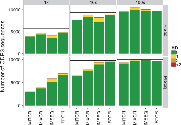
Accuracy of CDR3 sequences retrieved by several pipelines from simulated HTS datasets. ART was used to simulate 150 bp HiSeq 2500 (top-row) and 250 bp MiSeq (bottom row) paired-end reads. The fold coverage of every dataset, was 1×, 10× or 100×. Due to sampling only a subset of the in silico CDR3 sequences was spanned by one or more reads (horizontal black lines) and could potentially be retrieved. The merged paired-end reads of HiSeq 2500 and MiSeq had an average Phred quality of 37 and 35, respectively, and a substitution error rate of ∼1%. We ran the analysis on several independent datasets and here show one representative example. Number of mismatches with the most similar true CDR3 sequence of the same length

Table 1.

Average precision and recall of the pipelines on all HiSeq 2500 and MiSeq datasets (1×, 10× and 100× coverages combined)

Pipeline	HiSeq 2500		MiSeq
	Precision (%)	Recall (%)	Precision (%)	Recall (%)
TCRklass	63.7	84.8	60.0	74.5
MiTCR	98.4	81.7	98.4	66.5
MiXCR	93.5	88.2	95.8	75.9
IMSEQ	89.7	79.6	94.1	87.1
RTCR	98.4	92.0	97.2	94.6

We compared the CDR3 sequences reported by the pipelines to those of the ‘true’ simulated TCRB repertoire (Fig. 3). The horizontal line in each panel depicts the number of CDR3 sequences of the ‘true’ repertoire that was represented by one or more reads that spanned the CDR3 region. If a bar falls below this line, the pipeline underpredicted the number of CDR3 sequences in the HTS dataset; conversely, if a bar is higher than the black line, the number of CDR3 sequences was overpredicted by the pipeline. To visualize the quality of the reported list of CDR3 sequences, we colored the bars reflecting the fraction of the reported sequences that perfectly matched a CDR3 in the ‘true’ repertoire (green) that had one mismatch with the most similar true CDR3 sequence (yellow), two mismatches (orange) or more than two mismatches (red). All pipelines, except TCRklass, tend to underreport the true number of sequences. The number of clones reported by RTCR is closest to the true diversity.

Since MiTCR had consistently high precision in all datasets, we attempted to increase the recall of MiTCR by changing several of its parameters. First, we tested the ‘save my diversity’ parameter, but this resulted in a loss of precision with hardly any increase in recall (data not shown). As MiTCR ascribes high quality TCR sequences as core sequences (ignoring the low quality sequences), using a ‘quality’ parameter to differentiate between them, we also attempted to increase the recall by lowering this parameter to 5. Although this lead to an increase in recall (data not shown), it markedly reduced the precision in the MiSeq data. This large difference between MiTCR and MiTCR_Q5 suggests the high precision of MiTCR results from discarding low quality sequences prior to its error correction.

With increasing coverage in the HiSeq 2500 datasets, the recall of RTCR increased from 84% to 97% while precision remained ∼98% (Figs. 2 and 3). In the MiSeq datasets, the recall of RTCR increased from 91% to 96% with increasing coverage, and precision ranged from 95% to 99%. Comparing the HiSeq 2500 and MiSeq results of RTCR, the recall varies more in the HiSeq datasets. Closer inspection showed that the recall dropped largely due to a failure to identify the CDR3 sequences in the reads. The recall of RTCR before error correction was ∼85% for the 1× coverage HiSeq 2500 datasets. So the lower recall in the HiSeq 2500 1× coverage datasets was not due to overzealous error correction. Different settings for Bowtie 2, or a different aligner, might increase the recall of RTCR.

In summary, the precision and recall of RTCR is more stable across different coverages and sequencers than that of TCRklass, MiTCR, MiXCR and IMSEQ. Importantly, RTCR had the highest recall in the low coverage datasets (1× and 10×), which markedly reduces sequencing costs, allowing more libraries to be sequenced.

Typically, researchers apply abundance and quality filters to their raw reads. We think these filters should not be used in combination with the advanced data-driven error correction of RTCR. To test the effect of such filters, we ran RTCR on one of the HiSeq 2500 10× simulated datasets, applying either an abundance or quality filter (Fig. 4). The abundance filter, which was applied after RTCR analysis, led to a large decrease in recall without a corresponding gain in precision. The quality filter, applied to raw reads (Fig. 4, right panel), strongly decreased recall, whereas the precision was either unaffected or decreased somewhat, because RTCR benefits from the additional information provided by low quality reads. Together these results demonstrate that quality and abundance filters can be detrimental to the precision and recall of RTCR.

Fig. 4.

Applying naive filters can negatively affect the accuracy of RTCR. Left panel, an abundance threshold was applied to clones reported by RTCR, discarding any clones with a count lower than the threshold. Right panel, to emulate discarding low quality reads, a quality filter was applied to raw sequence data before RTCR analysis, discarding all reads containing one or more bases in the CDR3 region with a Phred score below the threshold. One of the simulated HiSeq 2500 10× datasets was used for both panels

To test how well the pipelines recover CDR3 abundances, we compared the abundances of the reported CDR3 sequences to their true abundances in the reads (Fig. 5). Most pipelines accurately predicted the abundance of identified TCR sequences, but all pipelines missed some low frequency ($\le {10}^{-4}$) TCR sequences in the 10× HiSeq 2500 datasets. MiTCR also missed abundant ($\ge {10}^{-3}$) TCR sequences (black circles in Fig. 5), suggesting it is too ambitious in its error correction.

Fig. 5.

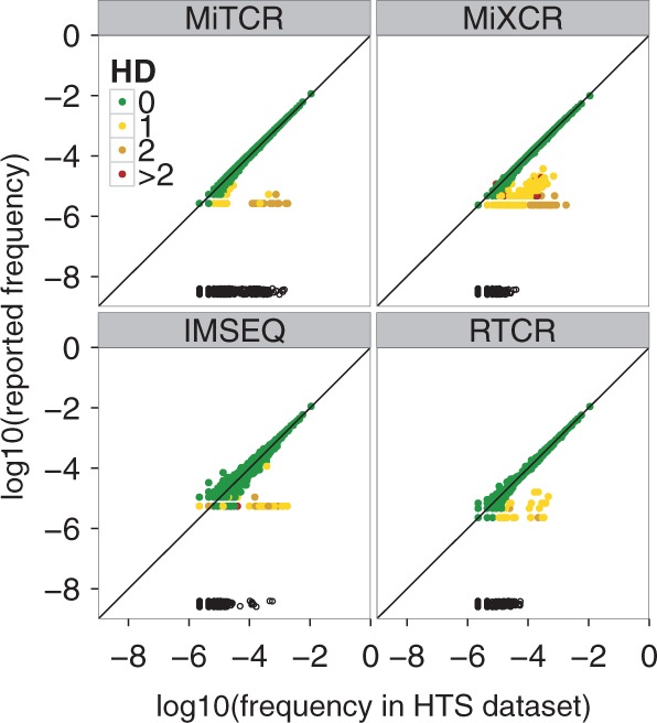
Quantitative TCR profiling of a HiSeq 2500 dataset, 10× coverage. CDR3 sequences (dots) retrieved by a pipeline are colored according to HD from the nearest true CDR3 sequence. Black open circles located at the bottom of each panel indicate missed CDR3 sequences. The reported frequency is the relative count assigned to a CDR3 sequence by a pipeline. The frequency of a CDR3 sequence in a HTS dataset is the ratio of reads spanning the particular CDR3 and the total number of reads spanning any CDR3

3.2 Analysis of a published TCR HTS dataset

Having tested TCRklass, MiTCR, MiXCR, IMSEQ and RTCR on simulated HTS datasets, where correctness of reported CDR3 sequences can be measured directly, we next compared the pipelines using a published TCR HTS dataset (Warren et al., 2011). Warren et al. (2011) obtained two blood samples of 20 ml each, 1 week apart, from a healthy adult male and sequenced these using an Illumina GAIIx Analyzer. Unfortunately, only the quality filtered reads, i.e. those having a CDR3 containing only bases with a quality score of at least Q30, were published. If the filtering removed many true TCR sequences, then this limits the benefit of the error correction of RTCR. To handle any remaining errors in the high fidelity reads, Warren et al. applied an abundance based filter, called D96, removing low-abundance sequence variants comprising a total of 4% of the reads. We analysed the published data of blood draws one and two with MiTCR, MiXCR, IMSEQ and RTCR, and compared the number of CDR3 sequences reported. We removed all out-of-frame CDR3 sequences and those containing a stop-codon (Warren et al., 2011).

Despite the many errors that may have been removed by the quality filtering, it is likely that different pipelines may not correct all errors. To test this hypothesis we visualized the sequence space around three representative abundant sequences in lane SRR060714 (Fig. 6). The sequence space around the chosen sequences had progressively less abundant sequences at higher HD, suggesting that the surrounding sequences might be erroneous variants (all three columns). The sequence (CSVPGQGGYEQYF) chosen for the first column broke this pattern with a medium abundant sequence (CSVPGQGVYEQYF) of about 600 reads, at HD 3. It is likely a correct sequence (similar to Fig. 1) because it was both abundant and assigned a different V gene (V29-1 instead of V20-1). All tested pipelines reported this sequence (Fig. 6, for every pipeline in the first column the rightmost circle from the center), but TCRklass and MiTCR also reported many (much) less abundant sequences. This example results suggest MiXCR, IMSEQ and RTCR are better at correcting PCR errors than MiTCR and TCRklass. However, MiXCR reported fewer clones than the uncorrected (‘Raw’) data and had a smaller overlap between the blood draws (Table 2), suggesting that this pipeline might not be correcting as many PCR errors as IMSEQ and RTCR.

Fig. 6.

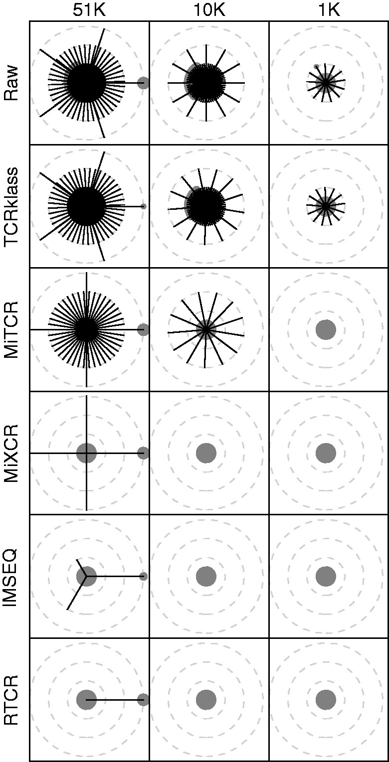
The sequence space of three abundant sequences from lane SRR060714 of Warren et al. (2011). The number above each column indicates the abundance of the chosen sequence in the ‘raw’ data, i.e. the CDR3 sequences identified by RTCR before error correction. Sequences (gray circles) within three HD of a central clonotype (columns) are connected (black lines). Circle area is the log-abundance ratio between a sequence and the total abundance of all sequences within the panel

Table 2.

CDR3 statistics of several analyses of Warren et al.’s Male 1 dataset

Pipeline	CDR3 BD 1	CDR3 BD 2	Overlap	Jaccard index
Raw	4 635 984	1 271 640	159 900	0.028
TCRklass	4 404 901	1 192 925	150 829	0.028
MiTCR	1 202 106	490 500	52 561	0.032
MiXCR	1 458 062	687 732	55 142	0.026
IMSEQ	879 442	363 206	38 355	0.032
RTCR	955 694	451 488	47 653	0.035
D96	494 796	352 139	45 150	0.056

The D96 counts and overlap are from Warren et al. (2011). Raw: the CDR3 sequences reported by RTCR before error correction. Sequences with stop-codon and out-of-frame sequences have been removed. BD, blood draw.

All pipelines reported more sequences than D96 (Table 2) and a smaller overlap (as measured by the Jaccard index) between the blood draws. Interestingly, IMSEQ reported considerably fewer CDR3 sequences, and had a lower overlap between the blood draws than RTCR, suggesting that IMSEQ removed true CDR3 sequences.

3.3 Analysis of a published barcoded TCR HTS data

A recent advance in HTS is the addition of unique molecular identifiers (‘barcodes’) to every template molecule (Kinde et al., 2011; Kivioja et al., 2012). With barcoded HTS data, many PCR and sequencing errors can be corrected by grouping reads with the same barcode together for consensus assembly (Shugay et al., 2014). This also enables direct quantification of the number of template molecules in the input (Kivioja et al., 2012) (i.e. the abundance), reducing the effect of PCR amplification bias on estimation of the true abundances of TCR sequences. RTCR supports the analysis of barcoded HTS data. First, RTCR collapses groups of sequences with the same barcode using consensus assembly. Next, RTCR runs the remainder of the pipeline as it would with non-barcoded data, combining barcode error correction with data-driven quality and frequency-based error correction. As RTCR has additional error correction on top of consensus assembly, it considers even small ‘barcode groups’ containing a single sequence, which are typically discarded by other pipelines.

To evaluate the performance of RTCR, we used a high quality and extremely deeply sequenced barcoded HTS dataset (‘Experiment 1’ from Egorov et al. (2015)), and compared the results to that of MiGEC, a pipeline designed to analyse barcoded data (Egorov et al., 2015; Shugay et al., 2014). Egorov et al. obtained blood from a 50-year-old male donor and divided it into eight replicas of ∼4000 peripheral blood mononuclear cells each. We used the barcoded TCRβ sequences (Illumina MiSeq 2× 150 bp paired-end reads) to compare both pipelines. MiGEC reported 236 clones of which most, 229, were also reported by RTCR. RTCR reported many more clones, 2717 in total across the eight replicas. This large difference is not unexpected, because RTCR recovers clones from barcode groups supported by only one sequence. The fact that RTCR recovers more clones that are reproducibly found in more than one library (Fig. 7), suggests that RTCR markedly outperforms MiGEC on recall because reproducible clones are more likely to be real. Importantly, reproducible clones are not guaranteed to have a correct sequence, as PCR errors are highly reproducible (Shugay et al., 2014), and their presence in multiple samples can be due to cross-sample contamination (Mamedov et al., 2013). Additionally, RTCR reported many more non-reproducible clones (2543) than MiGEC (151). However, given that there should be ∼2000 T cells present in each replica, and that about half of these are expected to be naive singletons, a diversity of several thousand clones across eight replicas is a very realistic result. In addition, the median Levenshtein distance from the non-reproducible clones to their closest neighbor was 6 (not shown), suggesting these clones are truly different. Together, these results suggest RTCR has a much higher recall than MiGEC. Unfortunately, we cannot quantify the precision and recall, because these measures cannot be reliably estimated in real data.

Fig. 7.

Capturing reproducible clones. Left panel, all distinct CDR3 sequences reported by MiGEC in each of the eight replicas of Egorov et al. (2015) were pooled and their frequencies of occurrence tallied, showing only those clones that occurred in more than one replica. Right panel, the same for RTCR

3.4 Performance

On an 8 core Intel Xeon 3.2Ghz 32GB RAM, RTCR takes ∼136 min (of which Bowtie 2 takes ∼63 min) to analyse a HiSeq 2500 dataset consisting of 10 million 150bp paired-end reads.

4 Conclusion

TCRs exhibit enormous diversity due to somatic recombination. The advent of HTS has enabled us to sequence large number of TCR sequences from an individual. However, HTS is marred by errors and given the TCR diversity it becomes difficult to distinguish between true TCR sequence and erroneous variants. We here present RTCR, a pipeline designed to accurately recover TCR sequences from error-prone HTS data. RTCR performs error correction using a statistical model and estimates the model parameters from the data, relieving the user from setting arbitrary parameters. Using simulations and experimental data, we demonstrate that RTCR can identify, and correct PCR and sequencing errors exhibiting consistently high precision and recall. The high accuracy of RTCR makes it well suited for estimation of repertoire diversity and for disease profiling. Especially in the lower coverage (1× and 10×) simulated datasets, RTCR outperformed all other pipelines. This means that RTCR has the potential to make the analysis of repertoire sequencing data more cost effective.

Funding

B.G. and A.C.A. were supported by the VIRGO consortium, which is funded by the Netherlands Genomics Initiative and by the Dutch government (FES0908). R.J.d.B. and A.P. were supported by the European Union Seventh Framework Program (FP7/2007-2013) under grant agreement 317040 (QuanTI).

Conflict of Interest: none declared.

References

- Alamyar E. et al. (2012). IMGT® tools for the nucleotide analysis of immunoglobulin (IG) and T cell receptor (TR) V-(D)-J repertoires, polymorphisms, and IG mutations: IMGT/V-QUEST and IMGT/HighV-QUEST for NGS In: Christiansen T. Frank, Tait T. D. Brian. Immunogenetics. Humana Press, Springer, Totowa, NJ, pp. 569–604. [DOI] [PubMed] [Google Scholar]
- Arstila T.P. et al. (1999) A direct estimate of the human αβ T cell receptor diversity. Science, 286, 958–961. [DOI] [PubMed] [Google Scholar]
- Bassing C.H. et al. (2002) The mechanism and regulation of chromosomal V(D)J recombination. Cell, 109, S45–S55. [DOI] [PubMed] [Google Scholar]
- Baum P.D. et al. (2012) Wrestling with the repertoire: the promise and perils of next generation sequencing for antigen receptors. Eur. J. Immunol., 42, 2834–2839. [DOI] [PubMed] [Google Scholar]
- Best K. et al. (2015) Computational analysis of stochastic heterogeneity in PCR amplification efficiency revealed by single molecule barcoding. Scientific reports, 5, 011411, Nature Publishing Group. [DOI] [PMC free article] [PubMed] [Google Scholar]
- Bolotin D.A. et al. (2012) Next generation sequencing for TCR repertoire profiling: platform-specific features and correction algorithms: new technology. Eur. J. Immunol., 42, 3073–3083. [DOI] [PubMed] [Google Scholar]
- Bolotin D.A. et al. (2013) MiTCR: software for T-cell receptor sequencing data analysis. Nat. Methods, 10, 813–814. [DOI] [PubMed] [Google Scholar]
- Bolotin D.A. et al. (2015) MiXCR: software for comprehensive adaptive immunity profiling. Nat. Methods, 12, 380–381. [DOI] [PubMed] [Google Scholar]
- Calis J.J., Rosenberg B.R. (2014) Characterizing immune repertoires by high throughput sequencing: strategies and applications. Trends Immunol., 35, 581–590. [DOI] [PMC free article] [PubMed] [Google Scholar]
- Cline J. et al. (1996) PCR fidelity of pfu DNA polymerase and other thermostable DNA polymerases. Nucleic Acids Res., 24, 3546–3551. [DOI] [PMC free article] [PubMed] [Google Scholar]
- Davis M.M., Bjorkman P.J. (1988) T-cell antigen receptor genes and T-cell recognition. Nature, 334, 395–402. [DOI] [PubMed] [Google Scholar]
- Egorov E.S. et al. (2015) Quantitative profiling of immune repertoires for minor lymphocyte counts using unique molecular identifiers. J. Immunol., 194, 6155–6163. [DOI] [PubMed] [Google Scholar]
- Freeman J.D. et al. (2009) Profiling the T-cell receptor beta-chain repertoire by massively parallel sequencing. Genome Res., 19, 1817–1824. [DOI] [PMC free article] [PubMed] [Google Scholar]
- Holt R.A., Jones S.J.M. (2008) The new paradigm of flow cell sequencing. Genome Res., 18, 839–846. [DOI] [PubMed] [Google Scholar]
- Huang W. et al. (2012) ART: a next-generation sequencing read simulator. Bioinformatics, 28, 593–594. [DOI] [PMC free article] [PubMed] [Google Scholar]
- Kinde I. et al. (2011) Detection and quantification of rare mutations with massively parallel sequencing. Proc. Natl. Acad. Sci. USA, 108, 9530–9535. [DOI] [PMC free article] [PubMed] [Google Scholar]
- Kivioja T. et al. (2012) Counting absolute numbers of molecules using unique molecular identifiers. Nat. Methods, 9, 72–74. [DOI] [PubMed] [Google Scholar]
- Klarenbeek P.L. et al. (2010) Human T-cell memory consists mainly of unexpanded clones. Immunol. Lett., 133, 42–48. [DOI] [PubMed] [Google Scholar]
- Kuchenbecker L. et al. (2015) IMSEQ-a fast and error aware approach to immunogenetic sequence analysis. Bioinformatics, 31, 2963–2971. [DOI] [PubMed] [Google Scholar]
- Langmead B., Salzberg S.L. (2012) Fast gapped-read alignment with Bowtie 2. Nat. Methods, 9, 357–359. [DOI] [PMC free article] [PubMed] [Google Scholar]
- Mamedov I.Z. et al. (2013). Preparing unbiased T-cell receptor and antibody cDNA libraries for the deep next generation sequencing profiling. Front. Immunol., 4, 456. [DOI] [PMC free article] [PubMed] [Google Scholar]
- Mora T. et al. (2010) Maximum entropy models for antibody diversity. Proc. Natl. Acad. Sci. USA, 107, 5405–5410. [DOI] [PMC free article] [PubMed] [Google Scholar]
- Murugan A. et al. (2012) Statistical inference of the generation probability of T-cell receptors from sequence repertoires. Proc. Natl. Acad. Sci. USA, 109, 16161–16166. [DOI] [PMC free article] [PubMed] [Google Scholar]
- Ndifon W. et al. (2012) Chromatin conformation governs T-cell receptor J β gene segment usage. Proc. Natl. Acad. Sci. USA, 109, 15865–15870. [DOI] [PMC free article] [PubMed] [Google Scholar]
- Nguyen P. et al. (2011) Identification of errors introduced during high throughput sequencing of the T cell receptor repertoire. BMC Genomics, 12, 106. [DOI] [PMC free article] [PubMed] [Google Scholar]
- Qi Q. et al. (2014) Diversity and clonal selection in the human T-cell repertoire. Proc. Natl. Acad. Sci. USA, 111, 13139–13144. [DOI] [PMC free article] [PubMed] [Google Scholar]
- Robins H.S. et al. (2009) Comprehensive assessment of T-cell receptor β-chain diversity in αβ T cells. Blood, 114, 4099–4107. [DOI] [PMC free article] [PubMed] [Google Scholar]
- Robins H.S. et al. (2010) Overlap and effective size of the human CD8+ T cell receptor repertoire. Sci. Transl. Med., 2, 47ra64. [DOI] [PMC free article] [PubMed] [Google Scholar]
- Shendure J., Ji H. (2008) Next-generation DNA sequencing. Nat. Biotechnol., 26, 1135–1145. [DOI] [PubMed] [Google Scholar]
- Shugay M. et al. (2014) Towards error-free profiling of immune repertoires. Nat. Methods, 11, 653–655. [DOI] [PubMed] [Google Scholar]
- Suessmuth Y. et al. (2015) CMV reactivation drives post-transplant T cell reconstitution and results in defects in the underlying TCRβ repertoire. Blood, 125, 3835–3850. [DOI] [PMC free article] [PubMed] [Google Scholar]
- Thomas N. et al. (2013) Decombinator: a tool for fast, efficient gene assignment in T-cell receptor sequences using a finite state machine. Bioinformatics, 29, 542–550. [DOI] [PubMed] [Google Scholar]
- Vander Heiden J.A. et al. (2014) pRESTO: a toolkit for processing high-throughput sequencing raw reads of lymphocyte receptor repertoires. Bioinformatics, 30, 1930–1932. [DOI] [PMC free article] [PubMed] [Google Scholar]
- Venturi V. et al. (2011) A mechanism for TCR sharing between T cell subsets and individuals revealed by pyrosequencing. J. Immunol., 186, 4285–4294. [DOI] [PubMed] [Google Scholar]
- Wang C. et al. (2010) High throughput sequencing reveals a complex pattern of dynamic interrelationships among human t cell subsets. Proc. Natl. Acad. Sci. USA, 107, 1518–1523. [DOI] [PMC free article] [PubMed] [Google Scholar]
- Warren R.L. et al. (2009) Profiling model t-cell metagenomes with short reads. Bioinformatics, 25, 458–464. [DOI] [PubMed] [Google Scholar]
- Warren R.L. et al. (2011) Exhaustive T-cell repertoire sequencing of human peripheral blood samples reveals signatures of antigen selection and a directly measured repertoire size of at least 1 million clonotypes. Genome Res., 21, 790–797. [DOI] [PMC free article] [PubMed] [Google Scholar]
- Woodsworth D.J. et al. (2013) Sequence analysis of T-cell repertoires in health and disease. Genome Med, 5, 98.. [DOI] [PMC free article] [PubMed] [Google Scholar]
- Yang X. et al. (2015) TCRklass: a new K-string–based algorithm for human and mouse TCR repertoire characterization. J. Immunol., 194, 446–454. [DOI] [PubMed] [Google Scholar]