Local versus global biological network alignment

Abstract

Motivation: Network alignment (NA) aims to find regions of similarities between species’ molecular networks. There exist two NA categories: local (LNA) and global (GNA). LNA finds small highly conserved network regions and produces a many-to-many node mapping. GNA finds large conserved regions and produces a one-to-one node mapping. Given the different outputs of LNA and GNA, when a new NA method is proposed, it is compared against existing methods from the same category. However, both NA categories have the same goal: to allow for transferring functional knowledge from well- to poorly-studied species between conserved network regions. So, which one to choose, LNA or GNA? To answer this, we introduce the first systematic evaluation of the two NA categories.

Results: We introduce new measures of alignment quality that allow for fair comparison of the different LNA and GNA outputs, as such measures do not exist. We provide user-friendly software for efficient alignment evaluation that implements the new and existing measures. We evaluate prominent LNA and GNA methods on synthetic and real-world biological networks. We study the effect on alignment quality of using different interaction types and confidence levels. We find that the superiority of one NA category over the other is context-dependent. Further, when we contrast LNA and GNA in the application of learning novel protein functional knowledge, the two produce very different predictions, indicating their complementarity. Our results and software provide guidelines for future NA method development and evaluation.

Availability and implementation: Software: http://www.nd.edu/~cone/LNA_GNA

Contact: tmilenko@nd.edu

Supplementary information: Supplementary data are available at Bioinformatics online.

1 Introduction

1.1 Motivation, background and related work

With advancements of high throughput biotechnologies, large amounts of protein-protein interaction (PPI) data have become available (Breitkreutz et al., 2008; Brown and Jurisica, 2007). Comparative analysis of PPI data across species is referred to as network alignment (NA). NA is gaining importance, since it can be used to transfer biological knowledge from well- to poorly-studied species, thus leading to new discoveries in evolutionary biology.

NA aims to find topologically and functionally similar (conserved) regions between PPI networks of different species (Faisal et al., 2015). Like genomic sequence alignment, NA can be local (LNA) or global (GNA). LNA aims to find small highly conserved subnetworks, irrespective of the overall similarity of compared networks (Fig. 1(a)) (Ciriello et al., 2012; Hu and Reinert, 2015; Mina and Guzzi, 2012; Pache and Aloy, 2012; Sharan et al., 2005). Since the highly conserved subnetworks can overlap, LNA typically results in a many-to-many node mapping between nodes of the compared networks—a node can be mapped to multiple nodes from the other network. In contrast, GNA aims to maximize overall similarity of the compared networks, at the expense of suboptimal conservation in local regions (Fig. 1(b)). GNA produces a one-to-one (injective) node mapping—every node in the smaller network is mapped to exactly one unique node in the larger network (Clark and Kalita, 2015; Hashemifar and Xu, 2014; Ibragimov et al., 2013; Kuchaiev and Pržulj, 2011; Malod-Dognin and Pržulj, 2015; Neyshabur et al., 2013; Patro and Kingsford, 2012; Saraph and Milenković, 2014; Seah et al., 2014; Singh et al., 2007; Sun et al., 2015; Todor et al., 2013; Vijayan et al., 2015).

Fig. 1.

Illustration of (a) LNA and (b) GNA

NA can also be categorized as pairwise or multiple, based on how many networks it can align. See Faisal et al. (2015) for a review of pairwise and multiple NA. Here, we focus on pairwise NA.

Given the different outputs of LNA and GNA, it is difficult to directly compare them. Hence, when a new NA method is proposed, it is compared only against existing methods from the same NA category. In this context, NA methods can be evaluated with measures of topological and biological alignment quality. An alignment is of good topological quality if it reconstructs the underlying true node mapping well (when this mapping is known) and if it conserves many edges. An alignment is of good biological quality if the mapped nodes perform similar function. LNA output is evaluated biologically but not topologically. This is because LNA outputs a many-to-many node mapping and thus to date it has not been clear how to compute edge conservation that has been defined only for one-to-one mapping (Saraph and Milenković, 2014). GNA is evaluated both topologically and biologically.

Despite the different output types of LNA and GNA, which makes their direct comparison difficult, the two NA categories have the same ultimate goal: to transfer functional knowledge from well- to poorly-studied species, thus redefining the traditional notion of sequence-based orthology to network-based orthology. For this reason, we introduce the first ever comparison of LNA and GNA.

1.2 Our approach and contributions

In the process of developing our novel framework for a fair comparison of LNA and GNA (Fig. 2), we do the following.

Fig. 2.

Summary of our LNA versus GNA evaluation framework, consisting of the following steps: (1) Input: networks from different species containing different types of PPIs. Note that for this network set, we do not know the true node mapping. Thus, we analyze an additional set of networks with known true node mapping. (2) Network comparative analysis: using prominent LNA or GNA methods (as listed) to align networks across different species. During the alignment construction process, we set each method’s node cost function (see Section 2.3) to use topological information only, sequence information only, or combined topological and sequence information. (3) Output: many-to-many node mapping for LNA or one-to-one node mapping for GNA. (4) Evaluation: measuring topological and biological quality of each alignment. (5) Results: fair comparison of LNA and GNA, and novel protein function prediction

1. We evaluate 10 prominent LNA and GNA methods.

2. We evaluate the NA methods on both synthetic networks with known true node mapping and real-world networks with unknown true node mapping. For the latter, we explore the impact on the results of using different PPI types and PPIs of varying confidence.

3. We develop new alignment quality measures that allow for a fair comparison of LNA and GNA, since such measures do not exist. We measure both topological and biological alignment quality.

4. We study the effect on the results of using only network topological information versus including also protein sequence information into the alignment construction process.

5. Our LNA versus GNA evaluation reveals the following. When using only topological information during the alignment construction process, GNA outperforms LNA both topologically and biologically; when sequence information is also included, GNA is superior to LNA in terms of topological alignment quality, while LNA is superior to GNA in terms of biological quality. Our approach is overall robust to the choice of PPI data, meaning that both different PPI types and confidence levels lead to consistent results in all cases topologically and in most cases biologically.

6. In addition to the thorough method evaluation, whose results provide guidelines for future NA method development, we apply the NA methods to predict novel protein functional knowledge. We find that LNA and GNA produce very different predictions, indicating their complementarity when learning new biological knowledge.

7. We provide a graphical user interface (GUI) for NA evaluation integrating the new and existing alignment quality measures.

2 Materials and methods

2.1 Data description

We analyze PPI networks with (1) known and (2) unknown true node mapping.

Networks with known true node mapping contain a high-confidence S.cerevisiae (yeast) PPI network with 1004 proteins and 8323 PPIs (Collins et al., 2007) and five noisy networks constructed by adding to the high-confidence network 5, 10, 15, 20 or 25% of lower-confidence PPIs from the same dataset (Collins et al., 2007); the higher-scoring lower-confidence PPIs are added first. We align the high-confidence network with each of the noisy networks. Since all networks contain the same nodes, we know the true node mapping. The high-confidence network is an exact subgraph of each noisy yeast network. This popular evaluation test has been adopted by many existing NA studies (Kuchaiev and Pržulj, 2011; Kuchaiev et al., 2010; Patro and Kingsford, 2012; Saraph and Milenković, 2014; Vijayan et al., 2015).

Networks with unknown true node mapping are PPI data from BioGRID (downloaded in November 2014) of four species: S.cerevisiae (yeast), D.melanogaster (fly), C.elegans (worm) and H.sapiens (human). For each species, we extract four PPI networks containing different interaction types and confidence levels: (i) all physical PPIs, where each PPI is supported by at least one publication (PHY₁), (ii) all physical PPIs, where each PPI is supported by at least two publications (PHY₂), (iii) only yeast two-hybrid physical PPIs, where each PPI is supported by at least one publication (Y2H₁) and (iv) only yeast two-hybrid physical PPIs, where each PPI is supported by at least two publications (Y2H₂). We vary the PPI type (all physical interactions, most of which are obtained by AP/MS, versus Y2H only) to test the robustness of our approach to this parameter. We vary PPI confidence levels because PPIs supported by multiple publications are more reliable than those supported by only a single publication (Cusick et al., 2009). For each network, we extract and use its largest connected component (Supplementary Section S1 and Supplementary Table S1).

2.2 Network aligners evaluated in our study

To evaluate LNA against GNA, we choose most of the recent pairwise LNA and GNA methods that have publicly available and relatively user-friendly software. This results in four LNA methods and six GNA methods: NetworkBLAST (Sharan et al., 2005), NetAligner (Pache and Aloy, 2012), AlignNemo (Ciriello et al., 2012) and AlignMCL (Mina and Guzzi, 2012) from the LNA category; and GHOST (Patro and Kingsford, 2012), NETAL (Neyshabur et al., 2013), GEDEVO (Ibragimov et al., 2014), MAGNA++ (Vijayan et al., 2015), WAVE (Sun et al., 2015) and L-GRAAL (Malod-Dognin and Pržulj, 2015) from the GNA category. An exception to the above guidelines is NetworkBLAST—despite being an early LNA method, NetworkBLAST still remains a popular LNA baseline. All methods are described in Supplementary Section S2 and Supplementary Table S2, and their parameters that we use are shown in Supplementary Table S3.

2.3 Aligners’ node cost functions

All considered NA methods construct their alignments by first computing pairwise similarities between nodes from different networks via a node cost function (NCF). One can compute node similarities by accounting for: (i) topological information only (T) in order to measure how well the (extended) network neighborhoods of two nodes match, (ii) sequence information only (S) in order to measure the extent of sequence conservation between the nodes or (iii) combined topological and sequence information (T&S). We study the effect on alignment quality of using only topological information versus also using sequence information in NCF.

We evaluate each aligner for each of the three above cases. The exceptions are NetworkBLAST, NetAligner, NETAL and GEDEVO, for the following reasons. Regarding NetworkBLAST and NetAligner, they only allow for using sequence information within NCF. The two methods require E-value scores as input and it is unclear how to convert topological information into values that are at the same scale as the E-values. Regarding NETAL, its implementation failed to run when we tried to include sequence information into its NCF. Regarding GEDEVO, by design, its implementation allows for only using topological information and using this information in a specific format (i.e. as a 73-dimensional vector per node), where it is unclear how to convert sequence information into this particular format.

Topology- and sequence-based NCFs that we use within the different NA methods are discussed in Supplementary Section S3 and Supplementary Table S4. Given the topology- and sequence-based NCFs for two nodes from different networks, we compute the nodes’ combined (T&S) NCF as the linear combination of the individual NCFs: $NCF(T\text{\&}S)=\alpha \times NCF(T)+(1-\alpha )\times NCF(S)$. Initially, we have chosen $\alpha =0.5$ in order to equally balance between T and S. However, to give each method the best case advantage, our final strategy is to vary the value of α from 0.1 to 0.9 in increments of 0.1 and use the best α value in each test (for each method). Since using $\alpha =0.5$ and using the best α value lead to qualitatively identical results according to our analysis (as we will show in Section 3), for simplicity, henceforth, we only report the results when using the best α value for T&S (unless otherwise noted).

2.4 Evaluation of alignment quality

Next, we discuss measures that we use to evaluate topological (Section 2.4.1) and biological (Section 2.4.2) alignment quality. We introduce the following definitions. Let f be an alignment between two graphs $G_1(V_1,E_1)$ and $G_2(V_2,E_2)$. Given a node u from one graph, let f(u) be the set of nodes from the other graph that are aligned under f to u. Given a node set V, let $f(V)=\underset{v\in V}{\cup }f(v)$. Let $G{\prime }_1(V{\prime }_1,E{\prime }_1)$ and $G{\prime }_2(V{\prime }_2,E{\prime }_2)$ be subgraphs of G₁ and G₂ that are induced on node sets $f(V_2)$ and $f(V_1)$, respectively. We define conserved and non-conserved edges as follows. A conserved edge is formed by two edges from different networks such that each end node of one edge is aligned under f to a unique end node of the other edge. In other words, a conserved edge is composed of two edges from different networks that are aligned under f (Fig. 3(a)). A non-conserved edge is formed by an edge from one network and a pair of nodes from the other network that do not form an edge (i.e. that form a non-edge) such that each end node of the edge is aligned under f to a unique node of the non-edge (Fig. 3(b) and (c)).

Fig. 3.

Illustration of conserved and non-conserved edges. (a) A conserved edge is formed by two edges $(u,v)\in G_1$ and $(u\prime ,v\prime )\in G_2$ such that u is aligned to $u\prime$ and v is aligned to $v\prime$. A non-conserved edge is formed by (b) an edge $(u,v)\in G_1$ and a non-edge $(u\prime ,v\prime )\in G_2$ , or by (c) a non-edge $(u,v)\in G_1$ and an edge $(u,v)\in G_2$, such that u is aligned to $u\prime$ and v is aligned to $v\prime$. Nodes of the same color come from the same network. A solid line represents an edge. Nodes linked by a dashed line are aligned under f

2.4.1 Topological evaluation

First, we describe existing topological alignment quality measures, along with their drawbacks. Next, we propose new measures that are motivated by the drawbacks of the existing measures.

Existing measures. Recall that intuitively an alignment is of high topological quality if it reconstructs the underlying true node mapping well (when such mapping is known) and if it conserves many edges.

To evaluate how well an alignment reconstructs the true node mapping, node correctness (NC) has been widely used (Kuchaiev and Pržulj, 2011; Kuchaiev et al., 2010). To date, NC has been defined only for GNA, as the fraction of nodes from the smaller network that are correctly aligned (under injective mapping f) to nodes from the larger network with respect to the true node mapping. The reason that NC has not been defined for LNA is that with LNA, a node from the smaller network can be mapped to multiple nodes from the larger network, and thus, it is not clear how to measure the percentage of nodes from the smaller network that are correctly aligned. Hence, below, we generalize NC for both LNA and GNA. NC can only be used when the true node mapping is known.

To measure how well edges are conserved under an alignment, three measures have been used to date: edge correctness (EC) (Kuchaiev et al., 2010), induced conserved structure (ICS) (Patro and Kingsford, 2012), and symmetric substructure score (S³) (Saraph and Milenković, 2014). S³ has been shown to be superior to EC and ICS, since intuitively it not only penalizes alignments from sparse graph regions to dense graph regions (as EC does), but also, it penalizes alignments from dense graph regions to sparse graph regions (as ICS does). Hence, we only focus on S³. Like NC, S³ has been only defined in the context of GNA, as $\frac{\left|E_1^{*}\right|}{\left|E_1\right|+\left|E_2^{\prime }\right|-\left|E_1^{*}\right|}$, where $\left|E_1^{*}\right|$ is the number of edges from G₁ that are conserved by f (in this case, G₁ is the smaller of the two networks in terms of the number of nodes). The reason that S³ has not been defined for LNA is that with LNA that allows for many-to-many node mapping, it is not clear how to count conserved edges, since an edge from one network could be aligned to multiple edges from the other network. Hence, below, we generalize S³ to both LNA and GNA.

New measures. To address the above issues, we propose new measures.

(1) Precision, recall and F-score of node correctness (P-NC, R-NC and F-NC, respectively). NC, defined only for GNA, measures how well an alignment reconstructs the true node mapping. As such, NC evaluates the precision of the alignment—the percentage of the aligned node pairs that are also present in the true node mapping. However, the corresponding recall—the percentage of all node pairs from the true node mapping that are aligned under f—is not measured explicitly. This is because for GNA, recall has the same value as precision. On the other hand, with LNA, precision and recall could have different values. In order to generalize NC for both GNA and LNA, we propose P-NC, R-NC and F-NC. Let M be the set of node pairs that are mapped under the true node mapping. Let N be the set of node pairs that are aligned under f. P-NC is defined as $\frac{|M\cap N|}{\left|M\right|}$. R-NC is defined as $\frac{|M\cap N|}{\left|N\right|}$. As is typically done (Hripcsak and Rothschild, 2005), we use F-NC, the harmonic mean of P-NC and R-NC, to combine the two individual measures. We have also tried other ways of combining P-NC and R-NC, such as by computing their geometric mean, and the results from using the geometric mean are significantly correlated (P-value $<{10}^{-308}$) with the results from using F-NC. Therefore, henceforth, we report results for F-NC but not for the geometric mean. Like NC, our three new measures can only be used when the true node mapping is known.

(2) Generalized S³ (GS³). To generalize S³ for both GNA and LNA, we propose GS³ to count edge conservation under f, independent on whether f is injective or many-to-many. We define GS³ as the percentage of conserved edges out of the total of both conserved and non-conserved edges:

$$G{S}^3=\frac{N_c}{N_c+N_n},$$ (1)

where N_c and N_n are the numbers of conserved and non-conserved edges, respectively, computed as follows. $N_c=\sum _{uv\in E{\prime }_1}|\{(u\prime ,v\prime )|u\prime \in f(u),v\prime \in f(v),(u\prime ,v\prime )\in E{\prime }_2\left\}\right|$. N_n is the sum of $N_n^1$ (i.e. the number of non-conserved edges formed by aligning an edge from G₁ and a non-edge from G₂; Fig. 3(b)) and $N_n^2$ (i.e. the number of non-conserved edges formed by aligning a non-edge from G₁ and an edge from G₂; Fig. 3(c))). $N_n^1$ and $N_n^2$ can be computed using Equations 2 and 3, respectively. Clearly, for GNA, Equation 1 for GS³ is S³ itself.

$$N_n^1={\displaystyle \sum _{uv\in E_1^{\prime }}|}\{(u\prime ,v\prime )|u\prime \in f(u),v\prime \in f(v),u\prime \ne v\prime \left\}\right|-N_c.$$ (2)

$$N_n^2={\displaystyle \sum _{u\prime v\prime \in E_2^{\prime }}|}\{(u,v)|u\in f(u\prime ),v\in f(v\prime ),u\ne v\left\}\right|-N_c.$$ (3)

(3) NCV combined with GS³ (NCV-GS³). Recall that GS³ measures how well edges are conserved between $G{\prime }_1$ and $G{\prime }_2$. LNA could produce small conserved subgraphs, which could result in high GS³ score. This would mistakenly imply high alignment quality if we only rely on GS³. But if we adopt an additional criterion of what a good alignment is, namely high node coverage (NCV), which is the percentage of nodes from G₁ and G₂ that are also in $G{\prime }_1$ and $G{\prime }_2$ (i.e. $\frac{\left|V_1^{\prime }\right|+\left|V_2^{\prime }\right|}{\left|V_1\right|+\left|V_2\right|}$), then small conserved subgraphs with high GS³ would actually have low alignment quality with respect to NCV. Thus, we combine NCV and GS³ into NCV-GS³ to get a more complete picture of the actual alignment quality. We define NCV-GS³ as the geometric mean of the two individual measures, because we want at least one low alignment quality score to imply low combined score.

2.4.2 Biological evaluation

To evaluate the biological quality of LNA and GNA, we use two existing measures: Gene Ontology (GO) correctness (Kuchaiev and Pržulj, 2011; Kuchaiev et al., 2010; Neyshabur et al., 2013) and the accuracy of known protein function prediction (Faisal et al., 2014; Kuchaiev and Pržulj, 2011; Patro and Kingsford, 2012; Sharan et al., 2005). Many GO annotations are obtained via sequence comparison (Crawford et al., 2015). Using such data to evaluate alignments of NA methods that already use sequence information in NCF would lead to biased results (Kuchaiev and Pržulj, 2011). Therefore, we only use GO annotations that have been obtained experimentally.

(1) GO correctness (GC). This measure quantifies the extent to which protein pairs that are aligned under f are annotated with the same GO terms (Supplementary Section S4) (Kuchaiev et al., 2010).

(2) Precision, recall and F-score of known protein function prediction (P-PF, R-PF and F-PF, respectively). We make GO term prediction(s) for each protein from G₁ or G₂ that is annotated with at least one GO term through a multi-step process. First, we hide the protein’s true GO terms. Second, we find statistically significant alignments with respect to each of those GO terms. Third, we predict the protein’s GO terms based on the GO terms of its aligned counterpart(s) under f only from the statistically significant alignments. Fourth, after we make predictions for all proteins, we evaluate the precision, recall and F-score of the prediction results (i.e. P-PF, R-PF and F-PF, respectively) with respect to the true GO terms of the proteins. For details about this 4-step process, see Supplementary Section S4.

2.5 Application to novel protein function prediction

One application of NA is to predict novel function of proteins based on the annotations of their aligned counterparts under f. We use LNA and GNA in this context to find statistically significant alignments and make novel protein function predictions from such alignments (Supplementary Section S5).

3 Results and discussion

After we validate our alignment quality measures (Section 3.1), we use the measures to evaluate LNA against GNA on networks with known (Section 3.2) and unknown (Section 3.3) true node mapping.

3.1 Validation of the alignment quality measures

Here, we aim to evaluate whether our proposed alignment quality measures (and in particular F-NC and NCV-GS³; Section 2.4.1) are actually meaningful. In the process, we also evaluate the existing F-PF measure (Section 2.4.2). We focus on these three measures for reasons discussed in Sections 3.2.1 and 3.3.1. We evaluate the measures in the following context: If we keep decreasing quality of a known alignment, a good measure should recognize the decreasing alignment quality and consequently lead to decreasing scores. To test whether our measures show this behavior, we perform two tests.

First, we vary the noise level in a correct node alignment, which is simply the known mapping from a node set to itself (e.g. node a is mapped to node a, node b is mapped to node b, node c is mapped to node c and so on). Such node mapping is clearly independent of the network topology or the NA method. Specifically, starting with the correct mapping between nodes from the set of yeast networks with known true node mapping (Section 2.1), we introduce 0–100% of noise into this mapping (where the noise corresponds to the percentage of mismatched node pairs, such as node a being mapped to node c), resulting in 21 alignments of decreasing quality. Then, for each measure, we compute the scores of the 21 alignments. We observe the trend that indicates that all measures are meaningful: their scores decrease with increase in noise level, i.e. with decrease in alignment quality (Supplementary Fig. S1).

Second, we perform a similar test, except that now we introduce the noise into the network topology directly, prior to aligning with each NA method the high-confidence yeast network to its noisy versions. We perform two variations of this test: (i) we ensure that each noisy network matches the degree distribution of the high-confidence network and (ii) we impose no such constraint. Since both variations lead to same trends, we report results for variation 1 only. This analysis is truly meaningful only when using topological information alone in NCF (corresponding to T; Section 2.3), since it is the network topology that we introduce the noise into. Consequently, for T, a good measure should definitely lead to decreasing alignment quality scores with increase in noise level. On the other hand, this analysis could be biased when using at least some amount of sequence information in NCF (corresponding to T&S and S; Section 2.3), because even while increasing the noise in the network topology, NA methods could still be heavily guided by sequence-based node similarities. Consequently, for T&S and S, NA methods could lead to high alignment quality scores even at high topological noise levels, especially with respect to measures that account for how well the aligned nodes match, such as F-NC and F-PF. However, this behavior should not be a sign that such measures are not meaningful; instead, this behavior should reflect the bias of using sequence information in NCF in this analysis.

With this in mind, our results are as follows. For T, all measures show decreasing alignment quality scores with the increasing noise (Fig. 4), as good measures should. Hence, this validates the measures. GNA is more robust to noise than LNA, as the scores drop faster for LNA than for GNA as noise increases. Importantly, recall that F-NC and F-PF reflect the correspondence or functional similarity between the aligned nodes, and thus, alignments of high quality in terms of F-NC or F-PF are biologically meaningful and can consequently efficiently guide the transfer of biological knowledge between the aligned networks. Now, since for T, F-NC and F-PF scores are high at the lowest noise levels and low at the highest noise levels for all NA methods (Fig. 4), this implies that topological information alone considerably reflects the underlying biological information, with superiority of GNA over LNA at the (meaningful) lowest noise levels. For T&S and S, alignment quality scores again decrease with increase in noise level for all methods in terms of NCV-GS³, which is not surprising as this is an edge-based (rather than node similarity-based) measure of alignment quality. Here, LNA and GNA perform similarly; Fig. 4 and Supplementary Fig. S2). This behavior of NCV-GS³ even when using some sequence information in NCF only further validates this measure. For F-NC and F-PF, the node similarity-based measures, as expected (see above), the scores for all LNA methods and for most of the GNA methods do not always decrease with increase in noise level. That is, scores at lower noise levels (when the aligned networks are similar) are sometimes the same as scores at higher noise levels (when the networks are dissimilar). This behavior confirms that the NA methods rely more heavily on sequence information than on topological information when matching similar nodes. This leads to many sequence-similar aligned node pairs independent of the topological noise level and consequently to many nodes being aligned to themselves (leading to high F-NC) or to other functionally similar nodes (leading to high F-PF).

Fig. 4.

Validation of the representative newly proposed alignment quality measures, (a) F-NC and (b) NCV-GS³, when introducing increasing noise level from 0 to 100% into the high-confidence yeast network (from the set of networks with known true node mapping) prior to aligning the high-confidence network with its noisy versions, for each of the aligners, with respect to T and S. For T&S, see Supplementary Figure S2. Results for F-PF closely match those for F-NC and are thus not reported. If some of the analyzed four LNA and six GNA methods are missing in the given panel, that means that the given method cannot be run with the corresponding type of information used in NCF (T or S)

We perform an additional (third) test of whether the analyzed measures are insensitive to the edge order of the input networks (as good measures should be), and we validate that this is the case (Supplementary Section S6 and Supplementary Fig. S3).

3.2 Networks with known true node mapping

3.2.1 Relationships between different alignment quality measures

To fairly evaluate different NA methods, we first study relationships and potential redundancies of different alignment quality measures in order to select only non-redundant measures to fairly evaluate LNA against GNA (Supplementary Section S7.1).

For networks with known true node mapping, we use the six topological measures: P-NC, R-NC, F-NC, NCV, GS³ and NCV-GS³ (Section 2.4.1). We do not use biological measures (which are approximate measures of similarity or correspondence between aligned nodes; Section 2.4.2) because we know the true node mapping, i.e. the actual correspondence between nodes that a good aligner should reconstruct well. For all pairs of measures, we compute Pearson correlation coefficients across all alignments (Supplementary Section S7.1). Since all six measures are topological, we expect them to be highly (positively) correlated with each other. Indeed, we find that over all of T, T&S and S combined, 89 and 71% of all pairs of measures are significantly correlated for LNA and GNA, respectively, with 60% of all pairs being in the intersection of LNA and GNA (Fig. 5(a) and (b), Supplementary Fig. S4, and Supplementary Section S7.1). The six measures by definition naturally cluster into two groups, one group consisting of P-NC, R-NC and F-NC, measures that quantify how well the alignment captures the true node mapping, and the other group consisting of NCV, GS³ and NCV-GS³, measures that capture the size of the alignment. Since (by definition) the two groups of measures evaluate alignment quality from different perspectives, since in the first group F-NC combines P-NC and R-NC while in the second group NCV-GS³ combines NCV and GS³, since within each group the measures are somewhat redundant (in the sense that, according to our results, F-NC overall correlates well with each of P-NC and R-NC, and NCV-GS³ overall correlates well with each of NCV and GS³), and since (according to our results) NCV-GS³ correlates the best with F-NC among all of NCV, GS³ and NCV-GS³, henceforth, we focus on F-NC and NCV-GS³ as the most representative non-redundant measures.

Fig. 5.

Pairwise relationships (Pearson correlations) between the six topological alignment quality measures for LNA (a and c) and GNA (b and d), for networks with known true node mapping (a and b) and networks with unknown true node mapping (c and d), with respect to T. For equivalent results with respect to T&S and S, see Supplementary Figures S4 and S10 (Color version of this figure is available at Bioinformatics online.)

3.2.2 Comparison of LNA and GNA

To fairly evaluate LNA against GNA, we perform ‘best method’ and ‘all methods’ comparisons of the NA methods. By ‘best method’ comparison, we mean the following: to claim that LNA is better than GNA, at least one LNA method has to beat all four of the GNA methods. Analogously, to claim that GNA is better than LNA, at least one GNA method has to beat all four of the LNA methods. If none of the two conditions are met, then we say that neither LNA nor GNA is superior. By ‘all methods’ comparison, we mean the following: to claim that LNA is better than GNA, each of the four LNA methods has to beat all four of the GNA methods. Analogously, to claim that GNA is better than LNA, each of the four GNA methods has to beat all four of the LNA methods. If none of the two conditions are met, then we say that neither LNA nor GNA is superior. We perform each of the ‘best method’ and ‘all methods’ comparisons with respect to each of T, T&S, S and B, where B is the best-case scenario, i.e. the best of T, T&S and S. Namely, given two networks and an NA method, three alignments will be produced, one for each of T, T&S and S. Then, B is the best of the three alignments with respect to the given alignment quality measure (different quality measures might identify different alignments as B out of T, T&S and S).

Here, we report our findings for the ‘best method’ comparison, while we provide results for the ‘all methods’ comparison in the Supplement. We focus on the ‘best method’ comparison for two reasons. First, we believe that the ‘best method’ comparison is more relevant than the ‘all methods’ comparison. This is because in order to properly answer which of LNA and GNA is superior, what matters is to find the best of all considered LNA methods and the best of all considered GNA methods and compare the resulting best methods only. That is, it might not be good to insist that even the worst LNA method beats the best GNA method (or vice versa), as this could severely weaken the comparison between LNA and GNA, especially if the worst LNA (or GNA) method is simply a poor-performing approach. Second, results for the two comparison types are qualitatively similar, which further strengthens our findings.

We find the following. Overall, for the ‘best method’ comparison, GNA is superior to LNA in all cases, for each of T, T&S, S and B (Figs 6 and 7, and Supplementary Fig. S5). Again, similar results hold for the ‘all methods’ comparison (Supplementary Fig. S5). When we zoom into these results in more detail to identify the best of all methods considered in our study (Fig. 7 and Supplementary Figs S6 and S7) , we find that AlignMCL is the best of all considered LNA methods, while MAGNA++ and WAVE are the best of all considered GNA methods. For details, see Supplementary Section S7.2; we provide this discussion in the Supplement since identifying the best particular method(s) is not a key question of our study. Further, we note that both LNA and GNA are more robust to the choice of networks to be aligned when some sequence information is used in NCF (i.e. with respect to T&S and S) than when only topological information is used (i.e. with respect to T), as supported by smaller standard deviations in Figure 7(b) and (c) compared to Figure 7(a).

Fig. 6.

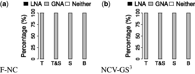
Overall ‘best method’ comparison of LNA and GNA for networks with known true node mapping with respect to (a) F-NC and (b) NCV-GS³ alignment quality measures, for T, T&S, S and B. Each bar shows the percentage of the aligned network pairs (over both considered alignment quality measures combined) for which LNA is superior (black), GNA is superior (grey), or neither LNA nor GNA is superior (white). For detailed results, see Figure 7 and Supplementary Figure S5

Fig. 7.

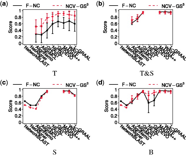
Detailed comparison of LNA and GNA for networks with known true node mapping with respect to F-NC and NCV-GS³ alignment quality measures, for (a) T, (b) T&S, (c) S and (d) B. Each point represents alignment quality of the given NA method averaged over all network pairs, and each bar represents the corresponding standard deviation. A missing point indicates that the given NA method cannot use the corresponding type of information in NCF and thus no result is produced

All results reported in Sections 3.1 and 3.2 correspond to using the best α value in NCF for T&S (Section 2.3). Using $\alpha =0.5$ to equally balance between topological and sequence information in NCF leads to comparable results (Supplementary Figs S8(a), (b) and S9), which further strengthens our findings. In general, we find that when a given NA method is run in the T&S mode, using any α in the [0.1,0.9] range leads to similar topological and biological alignment quality (Supplementary Fig. S8(a) and (b)).

3.2.3 Summary

For this network set, GNA is superior to LNA. AlignMCL is superior to all considered LNA methods. MAGNA++ and WAVE are superior of all considered GNA methods.

3.3 Networks with unknown true node mapping

3.3.1 Relationships of different alignment quality measures

Just as for networks with known true node mapping (Section 3.2.1), our first goal for four sets of networks with unknown true node mapping (Y2H₁, Y2H₂, PHY₁ and PHY₂, which encompass different species, PPI types and PPI confidence levels; Section 2.1) is to understand potential redundancies of different alignment quality measures and choose the best and most representative of all redundant measures for fair evaluation of LNA and GNA. All reported results are for all four sets of networks combined, unless otherwise noted. In Section 3.3.3, we break down the results per network set, in order to evaluate their robustness to the choice of network data in terms of PPI type and confidence level.

For the networks with unknown true node mapping, we use all seven measures: three topological (NCV, GS³ and NCV-GS³; Section 2.4.1) and four biological (GC, P-PF, R-PF and F-PF; Section 2.4.2). For all pairs of measures, we compute Pearson correlation coefficients across all alignments (Supplementary Section S8.1). Since by definition all seven measures naturally cluster into two groups (one group consisting of the three topological measures that capture the size of the alignment in terms of the number of nodes or edges, and the other group consisting of the four biological measures that quantify the extent of functional similarity of the aligned nodes), we expect within-group correlations to be higher than across-group correlations. Indeed, this is what we observe overall for both LNA and GNA with respect to each of T, T&S and S (Fig. 5(c) and (d), Supplementary Fig. S10, and Supplementary Section S8.1). Specifically, over all of T, T&S and S combined, 52 and 78% of all within-group correlations are significant for LNA and GNA, respectively, with 48% overlap between LNA and GNA. Similarly, 89 and 94% of all across-group correlations are non-significant for LNA and GNA, respectively, with 83% overlap between LNA and GNA.

These results (the majority of the within-group correlations being significant and the majority of the across-group correlations being non-significant) imply that topological and biological alignment quality are not significantly correlated, which clearly holds for both LNA and GNA. This was already observed by the existing GNA studies (Clark and Kalita, 2014; Crawford et al., 2015; Patro and Kingsford, 2012), which noted that the topological versus biological fit between aligned networks conflict to a larger extent than previously realized. An explanation could be that the discovery of the current experimental biological knowledge may have been guided by sequence-based (rather than network-based) analyses. Our findings support this hypothesis: in 99% of all cases, for the same NA method and the same pair of networks, alignments for T&S or S are superior to alignments for T in terms of biological quality. Similarly, it was already shown that functional similarities of aligned proteins reach their maximum for either T&S or S, but not for T (Malod-Dognin and Pržulj, 2015). If the current experimental biological knowledge is indeed biased towards sequence data, given that sequences and network topology can lead to complementary biological insights (Memišević et al., 2010), our above findings should not be surprising. Yet, we argue that network topology can be a valuable source of biological knowledge that can lead to novel insights compared to sequence data alone, as was already recognized by many of the existing NA studies and as our study additionally confirms. Namely, we have already shown in Section 3.1 that network topology reflects well the underlying biological information, and we additionally show in Section 3.5 that using some amount of topology can yield unique biological predictions that are not captured when using only sequences.

Going back to choosing the most representative measures, since by definition the two groups of measures (NCV, GS³ and NCV-GS³ versus GC, P-PF, R-PF and F-PF) evaluate alignment quality from different perspectives, since in the first group NCV-GS³ combines NCV and GS³ while in the second group F-PF combines P-PF and R-PF (and P-PF is also redundant to GC), since (according to our results) the measures within each of the two groups are overall well correlated and thus redundant to each other, and since (according to our results from Section 3.2.1) NCV-GS³ correlates the best with F-NC for networks with known true node mapping among all of NCV, GS³ and NCV-GS³, henceforth, we focus on NCV-GS³ and F-PF as non-redundant topological and biological measures, respectively.

3.3.2 Comparison of LNA and GNA

As in our analysis from Section 3.2.2, here we perform ‘best method’ and ‘all methods’ comparisons. For both comparison types, with respect to topological alignment quality, GNA is always superior to LNA for each of T, T&S, S and B (Fig. 8(a) and Supplementary Fig. S11). With respect to biological alignment quality, GNA is superior to LNA for T for majority of the cases, while LNA is superior to GNA for T&S, S and B (Fig. 8(b) and Supplementary Fig. S11). When we zoom into the above results (Supplementary Figs S12–S16) in order to identify the best NA method(s) among all methods considered in our study, we find that AlignNemo and AlignMCL are the best of all considered LNA methods, while for GNA, the best of all considered GNA methods varies depending on whether we are measuring topological versus biological alignment quality and depending on the type of information used in NCF. For details, see Supplementary Section S8.2; we provide this discussion in the Supplement since identifying the best particular method(s) is not a key question of our study.

Fig. 8.

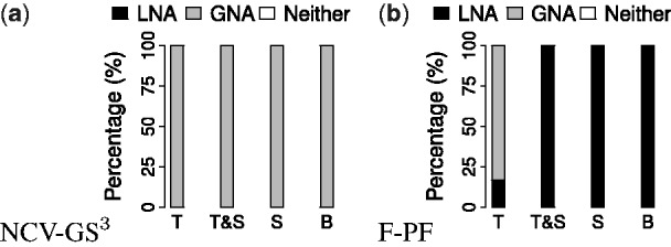
Overall ‘best method’ comparison of LNA and GNA for networks with unknown true node mapping from four different species (i.e. yeast, fly, worm and human) containing four different types of PPIs (i.e. Y2H₁, Y2H₂, PHY₁ and PHY₂) with respect to (a) NCV-GS³ and (b) F-PF alignment quality measures, for T, T&S, S and B. Each bar shows the percentage of the aligned network pairs for which LNA is superior (black), GNA is superior (grey), or neither LNA or GNA is superior (white). For detailed results, see Supplementary Figures S11 and S12

All results reported in Section 3.3 correspond to using the best α value in NCF for T&S. Using $\alpha =0.5$ leads to comparable results (Supplementary Figs S8(c), (d) and S17). In general, we find that when a given NA method is run in the T&S mode, using any α in the [0.1,0.9] range leads to similar topological and biological alignment quality (Supplementary Fig. S8(c), (d)).

3.3.3 Robustness to the choice of network data

We aim to study the effect on results of using different network sets (PHY₁, PHY₂, Y2H₁ and Y2H₂), in order to test the robustness of the results to the choice of PPI type and confidence level. For ‘best method’ comparison and each of T, T&S, S and B, with respect to topological alignment quality, results are always consistent across the different network sets (and they are consistent with the above reported results for all four network sets combined; Fig. 8). With respect to biological alignment quality, results for different network sets are consistent in 67% of all cases when varying PPI type and in 50% of all cases when varying PPI confidence level. Thus, our evaluation framework is robust to the choice of network data with respect to topological alignment quality and mostly robust with respect to biological alignment quality. For ‘all methods’ comparison and each of T, T&S, S and B, results are always consistent across the different network sets with respect to both topological and biological alignment quality (Supplementary Fig. S18).

3.3.4 Summary

Overall, when using only topological information in NCF, GNA outperforms LNA in terms of both topological and biological alignment quality. When adding sequence information to NCF, GNA is superior topologically, while LNA is superior biologically. The best of all considered LNA methods are AlignMCL and AlignNemo. The best of all considered GNA methods varies depending on whether one is measuring topological versus biological alignment quality and on the type of information used in NCF. Our evaluation is robust to the choice of network data with respect to topological alignment quality and mostly robust with respect to biological alignment quality.

The reason why GNA outperforms LNA in terms of topological alignment quality (meaning that GNA identifies larger amount of conserved edges and larger conserved subgraphs that LNA), irrespective of the type of NCF information used during the alignment construction process, could be due to the following key difference between the design goals of LNA and GNA. Namely, LNA aims to find small (on the order of a dozen nodes) but highly-conserved subnetworks, irrespective of the overall similarity between the compared networks. On the other hand, GNA aims to find a large conserved subgraph (though at the expense of matching local regions suboptimally), and typically it does so by directly optimizing edge conservation (and possibly other measures) while producing alignments. As such, simply by design, GNA might have an advantage over LNA in terms of the expected topological alignment quality, which our results confirm.

In terms of biological alignment quality, GNA again outperforms LNA for T. This indicates that when using within NCF only biological information encoded into network topology (i.e. when not using any biological information external to network topology, such as sequence information), GNA leads to better biological predictions than LNA. Also, in this case, the topological alignment quality results correlate well with the biological alignment quality results (as GNA is superior to LNA in both cases). However, when some amount of sequence information is included into NCF (corresponding to T&S and S), the topological alignment quality results do not correlate with the biological alignment quality results (as GNA is superior in the first case, while LNA is superior in the second case). The reason behind LNA’s superiority over GNA in terms of biological alignment quality for T&S and S could again be due to differences in their key design goals. Namely, unlike GNA, LNA uses the notion of the alignment graph to search for highly conserved subnetworks (Supplementary Section S2). When sequence information is used within NCF, nodes in this graph contain sequence-based orthologs, i.e. highly sequence-similar proteins from different networks. Since high sequence similarity often corresponds to high functional similarity, and since our measures of biological alignment quality are based on the notion of functional similarity between aligned proteins, by design LNA is ‘biased’ towards resulting in high biological quality whenever sequence information is used in NCF. However, LNA fails to produce biologically as good alignments as GNA when only topological information is used in NCF, as discussed above.

3.4 Running time method comparison

The results from Sections 3.2 and 3.3 compare the methods in terms of alignment accuracy. It is also important to compare the methods in terms of computational complexity, which we do here.

We run all NA methods on the same Linux machine with 64 CPU cores (AMD Opteron(tm) Processor 6378) and 512 GB of RAM. Since some NA methods (all LNA methods, as well as NETAL and WAVE GNA methods) can only run on one core while the others (GHOST, GEDEVO and MAGNA++ GNA methods) can run on multiple cores, for fair comparison, we run all methods on a single CPU core. An exception is GHOST, as its implementation still uses two threads even when its code is configured to use one core. We analyze the methods’ entire running times, both for computing node similarities and for constructing alignments. Also, we measure only running times needed to construct alignments, ignoring the time needed to precompute node similarities. We do the above when aligning worm and yeast PPI networks of Y2H₁ type (Table 1). We choose these networks because both are relatively small, and thus, the execution time for the slowest of all methods on a single core is reasonable (within one day). For any other network pair, running the slowest method on a single core would take much longer. Here, we choose the same value of α ($\alpha =0.5$) for all NA methods, in order to fairly compare their running times.

Table 1.

Representative running time comparison of the different NA methods, for each of T, T&S and S

Type	Method	Entire time (min)			Only time needed to construct alignments (min)
		T	T&S	S	T	T&S	S
LNA	NetworkBLAST	–	–	372.6	–	–	7.3
	NetAligner	–	–	368.2	–	–	2.35
	AlignNemo	375.5	450.3	370.0	4.9	0.4	0.4
	AlignMCL	377.0	452.1	365.2	1.6	1.75	1.7
GNA	GHOST†	78.2	438.5	435.3	7.5	9.5	10.7
	GHOST*	16.8	381.8	378.1	4.2	6.5	6.4
	NETAL	0.4	–	–	0.4	–	–
	GEDEVO†	2296.0	–	–	2290.6	–	–
	GEDEVO*	135.1	–	–	129.7	–	–
	MAGNA++†	287.8	768.9	690.7	224.6	225.2	221.7
	MAGNA++*	31.6	474.4	383.4	14.7	14.3	14.1
	WAVE	17.15	450.8	369.7	2.9	3.1	2.8
	L-GRAAL	432.9	378.3	374.0	61.0	6.4	2.1

Both the entire running times and only the running times for computing alignments are shown. For each method that is parallelizable (GHOST, GEDEVO and MAGNA++), its single-core version is marked with the ‘†’ character, and its 64-core version is marked with the ‘*’ character. All other methods are run on a single core. The ‘–’ character indicates that the given method cannot use the corresponding type of information in NCF and thus no result is produced.

We find that for the entire running time, for T, all GNA methods except GEDEVO and L-GRAAL run faster than the LNA methods; for T&S, GNA methods run similarly to LNA methods. For S, LNA is faster than GNA. For only the time needed to construct alignments, overall, LNA methods run faster than GNA methods for each of T, T&S and S (Table 1 and Supplementary Section S9).

In addition to the above single-core analysis, we give each method the best-case advantage, by running the parallelizable methods (GHOST, GEDEVO and MAGNA++ GNA methods) on multiple cores; we use as many cores as possible with the given method implementation, where 64 cores is the maximum imposed by our machine. We show these results also in Table 1. As expected, running the three NA methods on multiple cores indeed speeds up the methods’ running times. We do not necessarily see a linear decrease in running time with the increase in the number of cores, as not all parts of the given method are parallelizable.

Our results for the best-case, multi-core analysis are as follows. For the entire running time, for T, GNA runs faster than LNA. For T&S and S, unlike in the above single-core analysis where LNA is comparable or superior to GNA, GNA is now always comparable (if not even superior) to LNA. For only the time needed to construct alignments, LNA mostly remains faster than GNA (Table 1 and Supplementary Section S9).

3.5 Novel protein function predictions

Finally, we contrast LNA against GNA in the context of learning novel protein functional knowledge. We identify alignments in which the aligned network regions are significantly functionally similar according to known functional knowledge. Then, from such alignments, we predict novel functional knowledge in currently unannotated network regions whenever such regions are aligned to functionally annotated network regions (Section 2.5). Here, we choose the same value of α ($\alpha =0.5$) for all NA methods, in order to fairly compare the prediction results between LNA and GNA.

We find that LNA and GNA produce very different predictions, indicating their complementarity when learning new knowledge. Of the predictions made by all (LNA or GNA) methods for all of T, T&S and S, significant portion come from LNA only or GNA only, and only 10.4% come from both LNA and GNA (Fig. 9(a)).

Fig. 9.

Overlap of unique novel protein function predictions between (a) LNA and GNA over all of T, T&S and S combined, (b) T, T&S and S for GNA. See Supplementary Figure S19 for overlap of unique novel protein function predictions between T, T&S and S for LNA

We zoom into the above results for each of LNA (Supplementary Fig. S19) and GNA (Fig. 9(b)) to study the effect on the prediction results of using different types of information in NCF. We aim to test whether using some amount of topological information in NCF (corresponding to T or T&S) can yield unique predictions that are not captured when using only sequence information in NCF (corresponding to S). If so, this would confirm that additional biological knowledge is encoded in network topology compared to sequence data. Indeed, this is what we observe, for each of LNA and GNA: most predictions are unique to the different types of NCF information. Thus, network topology and sequence information complement each other when learning new biological knowledge.

3.6 User-friendly GUI plus source code

We make publicly available our software for NA evaluation (http://www.nd.edu/~cone/LNA_GNA). The software provides an intuitive GUI and python source code for any platform. For details, see Supplementary Section S10 and Figure S20.

4 Conclusions

In this paper, we systematically evaluate LNA against GNA. Our findings provide guidelines for researchers to properly demonstrate the superiority of a newly proposed NA (LNA or GNA) method. That is, we recommend that researchers evaluate the topological quality of a new NA method against state-of-the-art GNA (rather than only LNA) methods, irrespective of the type of information used in NCF, and that they evaluate the biological alignment quality of the new NA method against state-of-the-art GNA (rather than only LNA) methods when only T is used in NCF and against LNA (rather than only GNA) methods when S is also used in NCF.

NA is expected to continue to gain importance as more biological network data becomes available. This is because NA can be used to complement the across-species transfer of functional knowledge that has traditionally relied on sequence alignment (Clark and Kalita, 2014; Faisal et al., 2015). Thus, improvements upon the existing body of work on NA might be beneficial. For example, where GNA typically aims to ‘optimize’ topological alignment quality while LNA typically aims to ‘optimize’ biological alignment quality, ‘hybrid’ approaches that are designed to inherit the best from the two somewhat complementary worlds could lead to improved across-species knowledge transfer. Further, most of the existing NA methods are limited to undirected networks, while many biological network data are directed. So, NA methods that are able to handle directed networks are needed. Moreover, approaches that can align multiple networks at once might further improve the field of biological network comparison, and we have witnessed valuable recent efforts in this direction (Elmsallati et al., 2015; Faisal et al., 2015).

Funding

National Science Foundation [CAREER CCF-1452795, CCF-1319469 and IIS-0968529].

Conflict of Interest: none declared.

References

- Breitkreutz B.J. et al. (2008) The BioGRID interaction database: 2008 update. Nucleic Acids Res., 36, D637–D640. [DOI] [PMC free article] [PubMed] [Google Scholar]
- Brown K.R., Jurisica I. (2007) Unequal evolutionary conservation of human protein interactions in interologous networks. Genome Biol., 8, R95. [DOI] [PMC free article] [PubMed] [Google Scholar]
- Ciriello G. et al. (2012) AlignNemo: a local network alignment method to integrate homology and topology. Plos One, 7, e38107. [DOI] [PMC free article] [PubMed] [Google Scholar]
- Clark C., Kalita J. (2014) A comparison of algorithms for the pairwise alignment of biological networks. Bioinformatics, 30, 2351–2359. [DOI] [PubMed] [Google Scholar]
- Clark C., Kalita J. (2015) A multiobjective memetic algorithm for PPI network alignment. Bioinformatics, 31, 1988–1998. [DOI] [PubMed] [Google Scholar]
- Collins S. et al. (2007) Toward a comprehensive atlas of the physical interactome of Saccharomyces cerevisiae. Mol. Cell Proteomics, 6, 439–450. [DOI] [PubMed] [Google Scholar]
- Crawford J. et al. (2015) Fair evaluation of global network aligners. Algorithms Mol. Biol., 10, 1–17. [DOI] [PMC free article] [PubMed] [Google Scholar]
- Cusick M.E. et al. (2009) Literature-curated protein interaction datasets. Nat. Methods, 6, 39–46. [DOI] [PMC free article] [PubMed] [Google Scholar]
- Elmsallati A. et al. (2015) Global alignment of protein–protein interaction networks: a survey. IEEE/ACM Trans. Comput. Biol. Bioinf., doi: 10.1109/TCBB.2015.2474391. [DOI] [PubMed] [Google Scholar]
- Faisal F. et al. (2015) The post-genomic era of biological network alignment. EURASIP J. Bioinf. Syst. Biol., 2015, 1–19. [DOI] [PMC free article] [PubMed] [Google Scholar]
- Faisal F.E. et al. (2014) Global network alignment in the context of aging. IEEE/ACM Trans. Comput. Biol. Bioinf., 12, 40–52. [DOI] [PubMed] [Google Scholar]
- Hashemifar S., Xu J. (2014) HubAlign: an accurate and efficient method for global alignment of protein–protein interaction networks. Bioinformatics, 30, i438–i444. [DOI] [PMC free article] [PubMed] [Google Scholar]
- Hripcsak G., Rothschild A.S. (2005) Agreement, the F-measure, and reliability in information retrieval. J. Am. Med. Inf. Assoc., 12, 296–298. [DOI] [PMC free article] [PubMed] [Google Scholar]
- Hu J., Reinert K. (2015) LocalAli: an evolutionary-based local alignment approach to identify functionally conserved modules in multiple networks. Bioinformatics, 31, 363–372. [DOI] [PubMed] [Google Scholar]
- Ibragimov R. et al. (2013) GEDEVO: an evolutionary graph edit distance algorithm for biological network alignment. German Conf. Bioinf. (GCB), 34, 68–79. [Google Scholar]
- Ibragimov R. et al. (2014) Multiple graph edit distance: simultaneous topological alignment of multiple protein-protein interaction networks with an evolutionary algorithm. In: Proceedings of the 2014 Conference on Genetic and Evolutionary Computation, 277–284. [Google Scholar]
- Kuchaiev O., Pržulj N. (2011) Integrative network alignment reveals large regions of global network similarity in yeast and human. Bioinformatics, 27, 1390–1396. [DOI] [PubMed] [Google Scholar]
- Kuchaiev O. et al. (2010) Topological network alignment uncovers biological function and phylogeny. J. R. Soc. Interface, 7, 1341–1354. [DOI] [PMC free article] [PubMed] [Google Scholar]
- Malod-Dognin N., Pržulj N. (2015) L-GRAAL: Lagrangian graphlet-based network aligner. Bioinformatics, 31, 2182–2189. [DOI] [PMC free article] [PubMed] [Google Scholar]
- Memišević V. et al. (2010) Complementarity of network and sequence information in homologous proteins. J. Integr. Bioinf., 7, 135. [DOI] [PubMed] [Google Scholar]
- Mina M., Guzzi P.H. (2012). AlignMCL: Comparative analysis of protein interaction networks through Markov clustering. In: Proceedings of the 2012 IEEE International Conference on Bioinformatics and Biomedicine Workshops (BIBMW), pp. 174–181.
- Neyshabur B. et al. (2013) NETAL: a new graph-based method for global alignment of protein–protein interaction networks. Bioinformatics, 29, 1654–1662. [DOI] [PubMed] [Google Scholar]
- Pache R.A., Aloy P. (2012) A novel framework for the comparative analysis of biological networks. Plos One, 7, e31220. [DOI] [PMC free article] [PubMed] [Google Scholar]
- Patro R., Kingsford C. (2012) Global network alignment using multiscale spectral signatures. Bioinformatics, 28, 3105–3114. [DOI] [PMC free article] [PubMed] [Google Scholar]
- Saraph V., Milenković T. (2014) MAGNA: maximizing accuracy in global network alignment. Bioinformatics, 30, 2931–2940. [DOI] [PubMed] [Google Scholar]
- Seah B.S. et al. (2014) DualAligner: a dual alignment-based strategy to align protein interaction networks. Bioinformatics, 30, 2619–2626. [DOI] [PubMed] [Google Scholar]
- Sharan R. et al. (2005) Conserved patterns of protein interaction in multiple species. Proc. Natl. Acad. Sci. U. S. A., 102, 1974–1979. [DOI] [PMC free article] [PubMed] [Google Scholar]
- Singh R. et al. (2007) Pairwise global alignment of protein interaction networks by matching neighborhood topology. Res. Comput. Mol. Biol., 4453, 16–31. [Google Scholar]
- Sun Y. et al. (2015) Simultaneous optimization of both node and edge conservation in network alignment via WAVE. In: Workshop on Algorithms in Bioinformatics (WABI), pp. 16–39.
- Todor A. et al. (2013) Probabilistic biological network alignment. IEEE/ACM Trans. Comput. Biol. Bioinf., 10, 109–121. [DOI] [PubMed] [Google Scholar]
- Vijayan V. et al. (2015) MAGNA++: maximizing accuracy in global network alignment via both node and edge conservation. Bioinformatics, 31, 2409–2411. [DOI] [PubMed] [Google Scholar]
Associated Data
This section collects any data citations, data availability statements, or supplementary materials included in this article.