

Abstract
The increasing availability of complete genome data is facilitating the acquisition of phylogenomic data sets, but the process of obtaining orthologous sequences from other genomes and assembling multiple sequence alignments remains piecemeal and arduous. We designed software that performs these tasks and outputs anonymous loci (AL) or anchored enrichment/ultraconserved element loci (AE/UCE) data sets in ready-to-analyze formats. We demonstrate our program by applying it to the hominoids. Starting with human, chimpanzee, gorilla, and orangutan genomes, our software generated an exhaustive data set of 292 ALs (∼1 kb each) in ∼3 h. Not only did analyses of our AL data set validate the program by yielding a portrait of hominoid evolution in agreement with previous studies, but the accuracy and precision of our estimated ancestral effective population sizes and speciation times represent improvements. We also used our program with a published set of 512 vertebrate-wide AE “probe” sequences to generate data sets consisting of 171 and 242 independent loci (∼1 kb each) in 11 and 13 min, respectively. The former data set consisted of flanking sequences 500 bp from adjacent AEs, while the latter contained sequences bordering AEs. Although our AE data sets produced the expected hominoid species tree, coalescent-based estimates of ancestral population sizes and speciation times based on these data were considerably lower than estimates from our AL data set and previous studies. Accordingly, we suggest that loci subjected to direct or indirect selection may not be appropriate for coalescent-based methods. Complete in silico approaches, combined with the burgeoning genome databases, will accelerate the pace of phylogenomics.
The era of using genome-scale data to reconstruct the evolutionary history of organismal groups has recently begun (Alföldi et al. 2011; Faircloth et al. 2012; Lemmon and Lemmon 2012; Lemmon et al. 2012; McCormack et al. 2012; Jarvis et al. 2014; Prum et al. 2015). Due to the increasing numbers of whole-genome data sets that are publicly available, it is now straightforward to use in silico methods to discover and design hundreds or thousands of new loci such as “anonymous loci” (ALs) (Karl and Avise 1993; Peng et al. 2009; Wenzel and Piertney 2015), exon-primed intron-crossing or “EPIC” loci (Palumbi and Baker 1994; Li et al. 2010), conserved nuclear exon loci (Li et al. 2007), anchored enrichment “AE” loci (Lemmon et al. 2012; Lemmon and Lemmon 2013), and ultraconserved element “UCE” loci (Faircloth et al. 2012; McCormack et al. 2012) for use in phylogenomic studies. Once loci are designed, NGS target-capture methods are employed to obtain orthologous sequences from many different individuals or species (e.g., Faircloth et al. 2012; Lemmon et al. 2012), which results in data sets with orders of magnitude more loci than in previous years.
Which locus class is best for a given phylogenomic study will largely depend on the type of study because the evolutionary properties of the aforementioned loci vary (Thomson et al. 2010). In studies of recently diverged populations or species, the researcher should use more variable markers such as ALs (Chen and Li 2001; Yang 2002; Rannala and Yang 2003; Jennings and Edwards 2005; Lee and Edwards 2008; Thomson et al. 2010; Bertozzi et al. 2012; Lemmon and Lemmon 2012) or introns (Li et al. 2010; Thomson et al. 2010). Because the flanking sequences of AE and UCE loci tend to exhibit much variation, these loci may also perform well in studies involving recent divergences (Faircloth et al. 2012; Lemmon et al. 2012; Smith et al. 2013). However, for studies involving deep divergences spanning tens or hundreds of millions of years, the researcher must resort to highly conserved loci such as conserved exons (Li et al. 2007; Thomson et al. 2010), AE loci (Lemmon et al. 2012), or UCE loci (Faircloth et al. 2012).
In phylogenomic studies involving populations or species that diverged recently or rapidly, coalescent theory predicts that neutral genomic loci will often have retained ancestral polymorphisms, which can lead to gene tree-species tree conflicts (Hudson 1983; Tajima 1983; Maddison 1997; Rosenberg 2002; Felsenstein 2004; Wakeley 2009). Contrary to posing a problem, these ancestral polymorphisms provide important information about the evolutionary history of populations or species, which can be exploited by the use of multilocus coalescent-based statistical analyses. Indeed, many studies have used this approach to obtain robust estimates of species trees and historical demographic parameters (e.g., Yang 2002; Rannala and Yang 2003; Jennings and Edwards 2005; Lee and Edwards 2008; Brito and Edwards 2009; Edwards 2009; Reilly et al. 2012). Of the aforementioned loci classes, ALs are optimal for inferring species trees and divergence times at shallow phylogenetic scales, as well as for estimating historical demographic parameters in phylogeography studies (Jennings and Edwards 2005; Thomson et al. 2010; Lemmon and Lemmon 2012). One of the main advantages ALs enjoy over other types of loci is that they are thought to satisfy the assumption of selective neutrality required in studies using neutral-coalescent methods of analysis. The reasons for this are twofold. First, because ALs are harvested from random genomic locations (Karl and Avise 1993), it is likely that they will be composed of nonfunctional DNA (Meader et al. 2010; Lindblad-Toh et al. 2011; Ponting and Hardison 2011), which is presumably not under selective pressure (Graur et al. 2013). Second, because functional elements occupy only a small portion of vertebrate genomes (e.g., 5% in humans) (Lindblad-Toh et al. 2011), chances are good that ALs will be far from sites that are maintained by selection. This is important because sites linked to functional elements experience indirect selection via genetic hitch-hiking (Maynard Smith and Haigh 1974; Kaplan et al. 1989) or background selection (Felsenstein 1974; Charlesworth et al. 1993). Although most intron sites or fourfold degenerate third codon positions in exons may experience single-base substitutions without consequence to the fitness of the organism (i.e., be selectively neutral in a sense), their tight linkage to sites under strong selection may keep them from fulfilling the neutrality assumption. This same argument can be applied to the flanking regions of AE and UCE loci because they are tightly linked to sites under severe purifying selection (Katzman et al. 2007). Despite this concern, McCormack et al. (2012) suggested that selection may not adversely affect species tree inferences based on UCE loci due to increased rates of lineage sorting, a hypothesis that has received empirical corroboration (Faircloth et al. 2012). However, estimates of effective population sizes based on genomic regions around conserved loci under purifying selection are expected to be reduced relative to more distant regions where “neutral” loci may be found (McVicker et al. 2009). The effects of selection may also adversely affect estimates of other population genetic parameters such as population divergences and gene flow.
NGS-based sequence-capture methods for acquiring large phylogenomic locus data sets (Faircloth et al. 2012; Lemmon et al. 2012; Lemmon and Lemmon 2013) represent the main option for most studies involving nonmodel organisms at the present time. Despite their advanced nature, these approaches still have hurdles that can impede many researchers from amassing large data sets (i.e., hundreds to thousands of loci for dozens to hundreds of individuals). First, these methods demand considerable technical expertise and access to laboratories containing specialized laboratory equipment for NGS-library preparation and sequence capture. Second, bioinformatics processing of NGS data into ready-to-analyze data sets is a daunting challenge to many. Fortunately, this situation will soon dramatically improve when acquiring complete whole-genome sequences becomes a practical option for many researchers. Indeed, a recent projection (O'Brien et al. 2014) suggests we can expect at least 10,000 sequenced vertebrate genomes in coming years. Thus, a demand will exist for sophisticated bioinformatics tools to meet the challenge of this surge in available genomes. For example, software that can scan a whole annotated genome sequence for the maximum number of “ideal” ALs—i.e., loci with the properties of being single-copy, presumably neutral, and genealogically independent from each other—or a set of target loci such as AE/UCE loci and then extract orthologous sequences from other nonannotated genomes will enable researchers to obtain ready-to-analyze data sets in mere minutes or hours instead of weeks or months. These anticipated advances will revolutionize phylogenomics and dramatically increase our knowledge of the tree of life.
We developed software that automatically constructs AL and anchor (AE/UCE) loci data sets from complete genome sequences. To validate the software, we used genome data for the major extant hominoid lineages (i.e., human, chimpanzee, gorilla, and orangutan). Not only are complete genome data available for the hominoids, but their phylogenomic history has been well studied (Ruvolo 1997; Chen and Li 2001; Yang 2002; Rannala and Yang 2003; Satta et al. 2004; Patterson et al. 2006; Steiper and Young 2006; Hobolth et al. 2007, 2011; Burgess and Yang 2008; Peng et al. 2009; Faircloth et al. 2012; Schrago 2014). The hominoid clade, therefore, represents an ideal system for evaluating the performance of our software.
Results
ALFIE: software for the acquisition of AE/UCE loci data sets
ALFIE for Anonymous/Anchor Loci FIndEr is a package containing several Python scripts that work together to find either the maximum number of single-copy, presumably neutral, and genealogically independent ALs or a set of targeted AE/UCE loci in complete genomes. The program, which is available at https://github.com/igorrcosta/alfie (and in the Supplemental Material), outputs ready-to-analyze files in a variety of formats, such as FASTA, interleaved NEXUS (Maddison et al. 1997) with commands for the software BEST (Liu 2008) and MrBayes (Huelsenbeck and Ronquist 2001) appended, and PHYLIP (Felsenstein 2005). These output files enable the researcher to immediately begin multilocus coalescent analyses to infer species trees or estimate historical demographic parameters, conduct supermatrix-based phylogenetic analyses, and perform single-locus phylogenetic analyses among others. The alfie.py script encapsulates all functions in an easy to use command-line interface. Additional details about the ALFIE package can be found in the Methods.
ALFIE may be used to generate data sets of either AL or anchor (AE/UCE) loci (Fig. 1). For AL data set generation (Fig. 1A), it is necessary to provide the complete genome for each individual or species in FASTA format and a general feature format (GFF) file with all features (e.g., all known protein-coding genes, regulatory elements, RNAs, etc.) of the genome that will be used as query. Only one annotated genome is required, and genomes from multiple individuals per species can be used. To minimize the risk of designing ALs that violate the single-copy assumption, genome files with all repetitive DNA masked as Ns should be used. The AL finding module's first step is to map the intergenic sequences (i.e., anonymous regions) while discarding all sequences with known functions plus their genetically linked flanking regions (Fig. 1A). The purpose of this step is to isolate segments of DNA whose sites are presumably neutral. Intergenic regions chosen for AL development should be distant enough, in terms of recombinational distances from known functional elements so that they are free from the indirect effects of selection (e.g., background selection and hitchhiking). A “recombinational distance” is a measure that incorporates local recombination rates, effective population sizes, and physical distances (Kaplan et al. 1989). However, owing to the intractability of using such local recombinational distances, a global value for the minimum physical distance (in base pairs) between an AL and an annotated genomic element can be determined by the user (Chen and Li 2001; Burgess and Yang 2008; Peng et al. 2009). The value input into this “distance filter” represents a tradeoff between the number of ALs recovered and the effective decoupling of anonymous DNA segments from functional genomic elements. The anonymous regions are then cut into consecutive segments of user-defined length, which we termed “candidate anonymous loci” (Fig. 1A).
Figure 1.
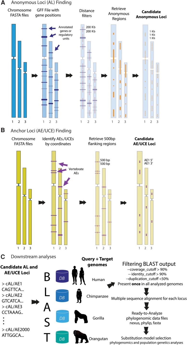
ALFIE software pipeline. (A) Anonymous loci (AL) finding module: User inputs complete genome sequences in a FASTA format and a general feature format (GFF) file for the query genome. Program first applies a user-defined “distance filter,” which removes all known functional elements + flanking sequences of user-specified lengths (purple color blocks). Remaining (presumably neutral) intergenic regions (orange color blocks), called candidate ALs, are retrieved and cut into consecutive segments of user-defined length and saved in FASTA files. (B) Anchor loci (AE/UCE) finding module: User inputs genome sequences in FASTA format. Program finds locations of target AEs/UCEs in a reference human genome with a coordinate file that currently contains 512 vertebrate AEs (included in package). Module retrieves flanking regions with user-defined length (e.g., 500 bp). User also specifies distance (in base pairs) between flanking sequences and their AEs/UCEs. Paired flanking sequences (i.e., candidate AE/UCE loci) are saved in FASTA files. (C) Downstream analyses: AL or AE/UCE candidate loci are used as query sequences in BLAST searches against target genomes. Single-copy loci are retained and subsequently aligned. A user-specified distance filter retains loci that are likely independent from other sampled loci. Each pair of AE/UCE flanking sequences is concatenated to form independent loci. Lastly, ALFIE outputs ready-to-analyze data sets.
For AE/UCE loci data set generation (Fig. 1B), the user must provide the complete genome for each individual or species in FASTA format (no annotated genomes required). The program maps all targeted AEs/UCEs in the query genome using a coordinate file and then retrieves both flanking sequences for each AE/UCE in the query genome. The size of the flanking sequence and the distance between each retrieved flanking sequence and its adjacent AE/UCE (both in base pairs) are defined by the user. These features allow users flexibility to obtain loci of desired lengths and levels of conservation since levels of site conservation generally decline with distance away from AEs/UCEs (Faircloth et al. 2012; Lemmon et al. 2012). We included in the program a coordinate file for the human genome that presently contains 512 vertebrate-wide AEs developed by Lemmon et al. (2012). In principle, coordinate files can contain the genomic locations for any set of target loci, and thus, we anticipate increasing the number and types of target loci in the future.
In the final step (Fig. 1C), the software uses candidate AL or AE/UCE loci as query sequences to conduct a BLAST search (Camacho et al. 2008) against all input genomes. The program only retains candidate loci present as a single copy in each sampled genome, and saves all sequences in FASTA files (Fig. 1C). Next, the pipeline conducts multiple sequence alignments for all candidate loci using ClustalW (Larkin et al. 2007), and paired AE/UCE flanking sequences are concatenated to form each individual locus. Loci found on the same chromosomes should be sufficiently separated from each other in order for their gene trees to be effectively independent of each other (Hudson and Coyne 2002; Jennings and Edwards 2005; Wakeley 2009; McCormack et al. 2012; Reilly et al. 2012; O'Neill et al. 2013; Leaché et al. 2015). Thus, the user must input a second distance threshold (in base pairs) separating sampled loci. Based on this distance threshold, the program excludes loci that may not be genealogically independent of the nearest loci found on the same chromosomes (Fig. 1C). After this last selection step, candidate ALs are considered “ideal” ALs because they are single copy, presumably neutral, independent from other sampled loci, and free of repetitive DNA and low complexity repeats (e.g., CpG sites). Similarly, candidate AE/UCE loci are considered to be single copy and genealogically independent of other sampled loci. The ALFIE pipeline finishes by outputting ready-to-analyze data sets in the various aforementioned formats.
Software validation: in silico phylogenomics of the hominoids
Running the Anonymous Loci Finder module on the annotated human genome and genomes from chimpanzee, gorilla, and orangutan with locus size set to 1 kb and both distance filters set to 200 kb (i.e., to find neutral independent loci; see Methods), program ALFIE required ∼3 h to generate a 292 AL data set (hereafter “AL 292”). In contrast, the Anchor Loci Finder module, which searched the same genomes for a total of 512 target vertebrate AE loci, ran much faster. With locus size set to 1 kb (i.e., 500 bp for each flanking sequence), the distance to the adjacent AE/UCE set to 0 bp, and the inter-locus distance filter set to 200 kb (to find independent loci; see Methods), program ALFIE needed just 13 min to produce a 242 AE data set (hereafter “AE 242”). To examine the effects of indirect selection on sites more distant from AEs/UCEs, we used the software to generate a second AE data set consisting of flanking sequences located 500 bp away from AEs, all other parameters being the same as the first data set. The program only required 11 min to output a data set consisting of 171 AE loci (hereafter “AE 171”).
An analysis of the distribution of all ALs in AL 292 by chromosome shows that these loci are scattered across the human genome (Supplemental Figs. S1A, S2; Supplemental Table S1). Although we specified a minimum physical distance of 200 kb separating loci found on the same chromosome, inspection of the location coordinates for these loci shows that in most cases the distances are much >200 kb with many loci separated by >1 Mb (Supplemental Table S1). The numbers of loci per chromosome were, unexpectedly, not distributed in proportion to the sizes of each chromosome: Chromosome 1 had fewer loci/bp, whereas Chromosomes 6, 13, and 18 had a higher concentration of loci (Supplemental Figs. S1A, S2; Supplemental Table S1). Instead, the heterogeneous spatial distribution of repetitive DNA (i.e., low complexity and interspersed repeats) across the genome better explains the relative amounts of presumably neutral DNA in each chromosome (Supplemental Fig. S1A). When regions of repetitive DNA are accounted for, the remaining amount of anonymous DNA strongly correlates with the numbers of candidate ALs per chromosome (Supplemental Figs. S1B, S2; Supplemental Tables S1, S2). The basic genomic characteristics of the AEs used in this study have been described elsewhere (Lemmon et al. 2012) and thus will not be discussed here.
Evaluation of 88 different DNA substitution models revealed that the HKY model best fit the majority of loci in each data set: 71% (208/292) of loci in AL 292, 50% (120/242) in AE 242, and 47% in AE 171 (Fig. 2A–C; Supplemental Tables S3–S5). The transition/transversion (Ti/Tv) rate ratio estimates also showed some consistency among data sets as the distribution of values for each data set peaked over Ti/Tv = 2 (Fig. 2D–F; Supplemental Tables S3–S5).
Figure 2.

Mutational profiles observed in three phylogenomic data sets obtained from human, chimpanzee, gorilla, and orangutan genomes. The data sets include 292 AL, 171 anchored enrichment (AE) loci, and 242 AE loci (for descriptions of each data set, see main text). (A–C) Distributions of nucleotide substitution models for each data set (for details about the different models, see Posada 2008). (D–F) Distributions of transition/transversion (Ti/Tv) rate ratios for each data set. Note, Ti/Tv values are only shown for loci that had a best-fitting nucleotide substitution model containing this parameter (i.e., 185, 133, and 230 loci, respectively). Also, five of the 171 AE loci and six of the 242 AE loci exhibited unusually high Ti/Tv values and thus were not included in these analyses. Source data are in Supplemental Tables S3 through S5.
Separate phylogenetic analyses for each locus in AL 292 generated a distribution of the three possible rooted tree topologies for human (H), chimpanzee (C), and gorilla (G) as follows: ((H, C), G) = 187/292 (64.0%), ((H, G), C) = 53/292 (18.2%), and ((C, G), H) = 52/292 (17.8%) (Supplemental Table S3). The AE 242 data set yielded the following gene tree topologies: ((H, C), G) = 133/242 (55.0%), ((H, G), C) = 39/242 (16.1%), and ((C, G), H) = 70/242 (28.9%) (Supplemental Table S4). The AE 171 topologies were: ((H, C), G) = 102/171 (59.6%), ((H, G), C) = 21/171 (12.3%), and ((C, G), H) = 48/171 (28.1%) (Supplemental Table S5).
Estimates for the ancestral effective population sizes NHC, NHCG, and NHCGO based on AL 292 yielded estimates for these three parameters of 42,000–59,000, 40,000, and 90,000–101,000, respectively (Fig. 3A; Supplemental Tables S6, S7). For comparative purposes and to assess the effects of number of loci, we also reanalyzed a previously published 53 AL data set for the hominoids; hereafter this data set will be referred to as “AL 53” (see Methods). Estimates of NHC, NHCG, and NHCGO based on AL 53 were 17,000–64,000, 41,000–49,000, and 31,000–92,000, respectively (Fig. 3A; Supplemental Tables S8, S9). Estimates of these same parameters using AE 171 data were 14,000–19,000, 26,000–27,000, and 114,000–128,000, respectively, whereas estimates based on AE 242 yielded 14,000–19,000, 24,000–25,000, and 132,000–145,000, respectively (Fig. 3A; Supplemental Tables S10–S13). We also estimated these parameters using only the 208 loci in AL 292 that fit the HKY model to see if the inclusion of other loci may have affected our results. The HKY-only results matched the results for the entire AL 292 data set (Supplemental Tables S14, S15).
Figure 3.

Bayesian estimation of ancestral effective population sizes and speciation times in the hominoids based on four phylogenomic data sets. (A) Inferred ancestral effective population sizes (Na) for the human–chimpanzee ancestor (NHC), human–chimpanzee–gorilla ancestor (NHCG), and human–chimpanzee–gorilla–orangutan ancestor (NHCGO). (B) Inferred speciation time in millions of years ago (Mya) between: human and chimpanzee lineages (τH-C), divergence leading to gorilla lineage (τHC-G), and divergence leading to orangutan lineage (τHCG-O). “AL 53” = 53 AL of Chen and Li (2001); “AL 292” = 292 AL; “AE 171” = 171 AE loci with each flanking sequence 500 bp from the adjacent AE; and “AE 242” = 242 AE loci with each flanking sequence 0 bp from the adjacent AE. Shown are posterior means and 95% credibility intervals for each parameter, which were estimated using five different sets of priors: P1 (blue), P2 (red), P3 (green), P4 (yellow), and P5 (orange; see Methods). Analyses for each parameter are contained within black boxes, and vertical dashed gray lines separate the results of each data set. Source data are in Supplemental Tables S6 through S13.
Our AL 292 data generated the following speciation time estimates: τHC = 3.8–4.1 million years ago (Mya), τHC-G = 6.1 Mya, and τHCG-O = 12.3–12.5 Mya. Our reanalysis of AL 53 generated estimates of 3.8–4.9 Mya, 5.9 Mya, and 12.5–14 Mya, respectively (Fig. 3B; Supplemental Tables S6–S9). Both AE data sets yielded speciation time estimates roughly twofold younger than those from the two AL data sets (Fig. 3B). Estimates based on AE 171 were τHC = 2.4–2.6 Mya, τHC-G = 3.4 Mya, and τHCG-O = 6.0–6.1 Mya, while AE 242 generated times of 2.1–2.2 Mya, 3.0 Mya, and 4.8 Mya, respectively (Fig. 3B; Supplemental Tables S10–S13). Estimation of these parameters using only the 208 AL loci that fit the HKY model likewise produced very similar estimates as those generated by the full data set (Supplemental Tables S14, S15).
Discussion
Distance thresholds vs. numbers of loci
The number of anonymous or anchor loci output by ALFIE is partly dependent on the input distance thresholds. For example, the use of 200-kb distance thresholds allowed ALFIE to generate 292 ALs (Supplemental Table S16). However, if the minimum distance to the nearest annotated genomic element is set to 500 kb, only six to 60 loci were output depending on the specified inter-AL threshold distance. When the distance to nearest gene is set to 700 kb, no loci were found.
Selection of appropriate distance thresholds represents one of the challenges to finding the maximum number of independent AL or AE/UCE loci in genomes. Even if the simplifying assumption of a single genome-wide recombination rate is made, optimal choices for threshold values will still largely be determined by the supposed value of Ne for the study group in question (Kaplan et al. 1989; Hudson and Coyne 2002). Thus, for groups (clades) with long-term Ne numbering in the hundreds of thousands or millions, the average physical distances required for ensuring that sampled loci are independent of each other or to sites under selection are expected to be shorter than for groups with smaller Ne. For example, if long-term Ne is large (>105), then ALFIE would likely output hundreds or thousands of ideal AL.
Maximum number of genealogically independent loci
ALFIE generated a data set consisting of 292 AL yet our theoretical analysis yielded an estimate of about 14,000 independent loci in the extant hominoid genome (see Methods). Why does such a large discrepancy exist? One obvious explanation is that the theoretical estimate includes all independent loci, while ALFIE uses stringent search criteria to select ideal AL. Thus, if the fraction of independent loci having the properties of being multicopy, being nonneutral, and containing repeat DNA was to be eliminated from consideration, then the remaining desirable fraction would likely number in the low thousands or hundreds, which is consistent with our empirical findings.
This finding raises an interesting question: How much of a genome is composed of neutral DNA? One of the initial steps of the ALFIE pipeline is to locate all regions far from any annotated element in order to find loci that are free from the direct and indirect effects of natural selection. Doing this analysis using a 200-kb distance threshold, we found that 247 Mb, or 8%, of the hominoid genome falls into this neutral DNA category (Supplemental Fig. S1B; Supplemental Table S2). By removing all repetitive and low-complexity repeat DNA from this fraction, we are left with only 18 Mb, or 0.6%, of the genome (Supplemental Table S2). Although these percentages will vary somewhat among species or clades owing to differences in the recombination landscapes of their genomes and long-term Ne values, these fractions are still likely to be quite small compared with the total amount of DNA classified as being nonfunctional. The implication of this is that most nonfunctional genomic sites are likely not free from the effects of natural selection and therefore may not be suitable for phylogenomic analyses that assume each locus is selectively neutral.
A more surprising result was our theoretical finding that the total number of independent loci in the human genome ranges between 1000 and 1400 (see Supplemental Methods). These numbers are an order of magnitude lower than our estimate for the hominoids owing to the much smaller Ne of humans than for the presumed sizes of the hominoid ancestral populations over the long term. Of these loci, only a fraction—perhaps numbering in the tens or low hundreds—likely represent single-copy, selectively neutral, and independent loci. This result has implications for human population genetic studies involving statistical procedures that assume each locus (or SNP) is neutral and independent. Indeed, studies that pseudoreplicate their loci or SNP number in statistical procedures that assume each locus or SNP is independent may lead to spurious inferences of species trees or historical demographic parameters. Thus, despite the vast sizes of many genomes, clearly there are limits to the numbers of genealogically independent loci that can be harvested.
DNA substitution patterns in neutral loci
Despite 88 different DNA substitution models evaluated during the model testing procedure, the HKY model (Hasegawa et al. 1985) best explained 71% of our ALs. It is not surprising that this model was so frequently chosen for ALs. First, the HKY model assumes unequal equilibrium base frequencies, which fits the overall low G + C content of 41% in the human genome (Graur et al. 2013). Second, the Ti/Tv rate ratio estimates for our presumably neutral loci span a narrow range with an average of 2.3, which matches previous estimates for nonfunctional human DNA with CpG sites discounted (Graur and Li 2000; Zhang and Gerstein 2003). Our model choice results together with the unimodally distributed Ti/Tv estimates for ALs (and AE loci as well) suggest that these loci largely evolved via a simple mechanism that gives rise to a transition bias (Wakeley 1996). This finding is significant because it provides evidence in support of the long-standing “rare tautomer hypothesis” by Watson and Crick (1953), which holds that spontaneous base substitutions, which are specifically transitions, arise via incorporation of rare base tautomers during DNA replication (Harris et al. 2003; Wang et al. 2011).
Hominoid species tree
In each of our ALFIE-generated data sets, the majority of rooted gene trees displayed the expected topology of a human–chimpanzee sister group relationship (Ruvolo 1997; Chen and Li 2001; Patterson et al. 2006; Hobolth et al. 2011; Faircloth et al. 2012; Schrago 2014). This constitutes strong evidence based on the majority-rule criterion that we recovered the correct hominoid species tree (Ruvolo 1997; Chen and Li 2001; Degnan and Rosenberg 2006). Moreover, our finding of equally frequent alternative topologies (∼18% each) in AL 292 also matches previous empirical studies (Ruvolo 1997; Patterson et al. 2006; Hobolth et al. 2011) and expectations of coalescent theory (Degnan and Rosenberg 2009; Wakeley 2009). However, gene tree distributions based on both AE data sets showed markedly unequal frequencies between the alternative topologies, which suggests that these distributions may be biased due to the long-term effects of selection.
Ancestral population sizes
In a reanalysis of AL 53, and using a prior mean of 12,500 for the gamma distribution, Yang (2002) estimated NHC to be 12,400. However, when he instead used a larger and more diffuse prior with a mean of 62,500, NHC increased to 33,000, suggesting the prior exerted much influence over the posterior probability distribution (Yang 2002, 2006). Rannala and Yang (2003) also analyzed AL 53 using similar methods and an informative prior identical to that used by Yang (2002), but their estimate of NHC was 24,600. Our results based on AL 53 and AL 292 data sets also revealed the same prior-driven pattern. However, the posterior means based on the larger data set (42,000–59,000) covered a narrower range than estimates from the smaller data set (17,000–64,000). This suggests that our use of diffuse priors together with fivefold more independent loci diminished the prior's influence on the posterior (Yang 2006). Estimates for our AE 171 and AE 242 data sets yielded estimates of NHC that ranged from 14,000–19,000, which are considerably lower than our AL 292 estimates. Moreover, they are also lower than other earlier estimates of NHC based on large data sets: 47,000 (Hobolth et al. 2011), 28,000–41,000 (Schrago 2014), and 99,000–122,000 (Burgess and Yang 2008; McVicker et al. 2009). That our AE estimates are so low is not unexpected, because these loci must be subject to some combination of direct and indirect natural selection, which would decrease effective population sizes. Given all discussed estimates, we conclude that our AE estimates do not reflect levels of neutral genetic variation and that our P1, P2, and P5 priors are not as realistic as our P3–P4 priors. Accordingly, we suggest that NHC was closer to about 54,000.
Yang's (2002) reanalysis of AL 53 using prior means of 12,500 and 62,500 yielded estimates of NHCG at 19,000 and 33,000, respectively. In a comparable analysis using the same data set, Rannala and Yang (2003) estimated NHCG to be 42,750. Our reanalysis of AL 53 revealed an effect of the priors, but the range of estimates (41,000–49,000) better reflects the estimate by Rannala and Yang (2003). Increasing the NHCG prior to 274,000 (P5) had only a minor effect on the posterior. Our AL 292 estimates for NHCG were all about 40,000 and thus proved robust against the use of different priors, while our AE estimates were, not unexpectedly, much lower (24,000–27,000). Schrago's (2014) estimate for this parameter (32,000) based on introns is comparable to our AE estimates. Given that intron loci likely experience some levels of direct and indirect selection, it is not surprising that his parameter value would be comparable to our AE results. In contrast, NHCG estimates of 52,000 and 55,000 were obtained by McVicker et al. (2009) and Burgess and Yang (2008), respectively, both of which better compare to our AL 292 estimates (about 40,000). These independent estimates again suggest that selection has reduced the effective population size of this ancestral population at our AE loci. Note, that if the NHCG estimate from Rannala and Yang (2003) is recalculated assuming a 21.2-yr-long generation time for the human–chimpanzee–gorilla ancestor obtained from Schrago (2014), then their estimate along with our AL 292 locus estimate suggest NHCG to be about 40,000.
In Rannala and Yang's (2003) reanalysis of AL 53, they estimated the NHCGO to be 24,750 based on a prior mean of 12,500. Our reanalysis of this data set produced NHCGO estimates ranging from 31,000–92,000 and shows the same prior-induced trend observed in the other population size parameters. Other estimates for NHCGO include 84,000 (based on neutral loci) (Burgess and Yang 2008), 84,000 (McVicker et al. 2009), 187,000 (Hobolth et al. 2011), and 272,098 (Schrago 2014). Analysis of our AL 292 locus data set also shows some influence of the priors, but compared to our AL 53 results, the range of estimates is narrower at 90,000–101,000. Despite increasing the prior mean of NHCGO to 274,000 in one analysis, we only observed a slight increase in the posterior mean. Our two AE data sets yielded estimates of this population size parameter ranging from 114,000–145,000, which are higher than those based on our AL 292 data set. However, given the substantial variation in estimates of this parameter (24,750–272,098), it is difficult to conclude which estimate best reflects the true value. As before, we believe the P1–P2 prior means for the ancestral population sizes are unrealistically low and P5 unrealistically high. Therefore, we favor our estimates based on the AL 292 data set and P3–P4 priors, which places NHCGO at about 100,000, because these data likely best meet the neutrality assumption and are apparently not being driven by poor priors.
Speciation times
Chen and Li (2001) estimated τHC to be 4.6 or 6.2 Mya depending on whether a 12- or 16-Mya time calibration, respectively, was applied to the root node (i.e., τHCG-O). In Yang's (2002) reanalysis of AL 53, he estimated τHC to be 5.3 or 4.6 Mya depending on whether an informative or diffuse gamma prior was used, respectively. Rannala and Yang (2003), who used the same data and similar methods to Yang (2002), instead arrived at an estimate of 4.3 Mya. Results of our reanalysis of AL 53, which are based on 10 and 18 Mya priors for τHCG-O, estimated τHC to be 3.8–4.9 Mya. Surprisingly, variation among these estimates was not due to the different divergence time priors but instead is attributable to different population size priors. Yang (2002) and Rannala and Yang (2003) discussed the correlations between these parameters. Our AL 292 data set yielded estimates of τHC ranging from 3.8–4.1 Mya, indicating the priors exerted little influence over the larger data set. Our estimates of τHC based on AL 292 are comparable with the majority of previous molecular studies: 4.9 Mya (Hasegawa et al. 1987), 4.6 Mya (based on diffuse prior) (Yang 2002), 4.3 Mya (Rannala and Yang 2003), 4.0 Mya (Burgess and Yang 2008), <5.4 Mya (Patterson et al. 2006), 4.1 Mya (Hobolth et al. 2007), 4.2 Mya (Hobolth et al. 2011), and 3.6–4.1 Mya (Schrago 2014). Interestingly, our two AE data set yielded substantially more recent NHC divergence times of 2.1–2.6 Mya, which, in light of the other estimates, must represent underestimates of the true divergence date. Although human–chimpanzee speciation may have been a demographically complicated and prolonged process lasting millions of years (Pilbeam and Young 2004; Patterson et al. 2006), our AL 292 estimates for τHC reinforce the predominant molecular viewpoint that gene flow cessation between the lineages, and hence speciation, occurred ∼4 Mya (Hobolth et al. 2007, 2011).
Chen and Li (2001) estimated τHC-G at 6.2 and 8.4 Mya depending on the assumed orangutan lineage divergence time of 12 or 16 Mya, respectively. In Yang's (2002) reanalysis of AL 53, he estimated τHC-G to be 6.5 and 6.9 Mya depending on which priors were used, whereas Rannala and Yang (2003) obtained an estimate of 6.0 Mya with the same data set. Our analyses of the AL 53 and AL 292 data sets generated estimates for τHC-G of 5.9 and 6.1 Mya, respectively, regardless of the priors. Our larger data set estimate of a 6.1-Mya gorilla divergence time agrees with the majority of previous molecular studies: 5.9 Mya (Hasegawa et al. 1987), 6.2 and 8.4 Mya (Chen and Li 2001), 6.5 Mya (based on diffuse prior) (Yang 2002), 6.0 Mya (Rannala and Yang 2003), 7.2 Mya (Satta et al. 2004), 8.6 Mya (Steiper and Young 2006), 6 Mya (Hobolth et al. 2007), 6.4 Mya (Burgess and Yang 2008), 9.5 Mya (McVicker et al. 2009), and 5.8–6.0 Mya (Schrago 2014). In contrast, both of our AE data sets suggest a far more recent gorilla divergence (3.0–3.4 Mya). Again, our AE data evidently underestimated, rather severely, a major speciation event in the hominoid species tree.
In their reanalysis of AL 53, Rannala and Yang (2003) estimated τHCG-O at 14 Mya, while our analysis of these data suggested this event occurred between 12.5–14 Mya depending on the priors. Our AL 292 data set produced a comparable but narrower range from 12.3–12.5 Mya, showing once again how little the priors influenced the posteriors. As with our τHC and τHC-G estimates, variation among estimates within data sets was due to a correlational effect attributable to different population size priors. Although two studies (Satta et al. 2004; Steiper and Young 2006) estimated τHCG-O to be ∼18 Mya, our estimate of ∼12.5 Mya agrees well with the majority of previous studies: 11.9 Mya (Hasegawa et al. 1987), 14 Mya (Goodman et al. 1998), 14 Mya (Rannala and Yang 2003), 14.6 Mya (Burgess and Yang 2008), 12 Mya (McVicker et al. 2009), 9–13 Mya (Hobolth et al. 2011), and 10.9–13.8 Mya (Schrago 2014). Estimates of the orangutan divergence based on our AE data sets were placed at only 4.8–6.1 Mya, which are half that of established estimates. Our preferred estimates for the ancestral effective population sizes and speciation times on the accepted hominoid species tree are shown in Supplemental Figure S3.
Benefits of hundreds or more of independent neutral loci
Because independent neutral loci represent independent samples of the coalescent process (Wakeley 2009), larger numbers of such loci are expected to produce more accurate and powerful estimates of species trees, ancestral population sizes, and speciation times (Pluzhnikov and Donnelly 1996; Jennings and Edwards 2005; Felsenstein 2006; Lee and Edwards 2008). Our empirical results provide strong evidence in support of these assertions. First, the posterior means based on AL 53 were markedly influenced by the priors, whereas the posteriors based on our 292-locus data set were less biased if affected at all. This is the same pattern observed in previous studies (Jennings and Edwards 2005; Lee and Edwards 2008), which had examined the posterior means and variances as a function of number of loci that had been randomly subsampled from the same data set. As Yang (2002, 2006) and Jennings and Edwards (2005) noted, it is of concern to know whether the posterior is sensitive to the prior in Bayesian population genetic analyses. In cases such as the present study in which a large amount of data dominate the posterior, the subjectivity of prior specification becomes less important particularly if diffuse priors are used (Yang 2002, 2006; Jennings and Edwards 2005).
Improved reliability of parameter estimates represents a second benefit of having more independent loci. When we contrast our parameter estimates based on AL 53 versus AL 292 loci, the Bayesian 95% credibility intervals based on the smaller data set are generally two- to threefold broader than the intervals associated with the larger data set (see Fig. 3). This mirrors the pattern found in several studies that had evaluated posterior variances as a function of the number of subsampled loci (Jennings and Edwards 2005; Lee and Edwards 2008; Smith et al. 2013). To our knowledge, this is the first time two independent data sets of drastically different numbers of loci (fivefold difference) have been compared to show the benefits of larger numbers of independent loci in phylogenomic studies.
While there is no doubt about the importance of the independent loci assumption in coalescent-based analyses, less clear are the consequences of violating the neutrality assumption. McVicker et al. (2009) presented evidence implicating indirect selection as the agent responsible for reducing effective population sizes of ancestral hominoids at genomic loci adjacent to conserved elements. With only one exception, our estimates of ancestral population sizes and speciation times in hominoids based on our AE data sets were not just substantially below those generated by our presumably neutral AL but also well below the ranges of previous estimates. Based on these empirical results, we suggest that AE loci—and by extension other loci that are subjected to direct or indirect natural selection such as UCE, EPIC, and exonic loci—may not sufficiently meet the neutrality assumption of coalescent-based methods, inducing systemic underestimation of population genetic parameters. Given the increasing ease of acquiring large phylogenomic data sets composed of different loci, as well as the desire to perform coalescent-based analyses, additional empirical and simulation studies are needed to study the effects of violating the neutrality assumption.
Methods
Software development
Our software is called the ALFIE package and is available at https://github.com/igorrcosta/alfie and in the Supplemental Material. It was developed in Python 2.7 using the Biopython library (Cock et al. 2009) and contains several Python scripts that work together to generate ready-to-analyze phylogenomic data sets from complete genome data. The program contains a module for finding the maximum number of ideal AL in a genome and a module for finding a set of genealogically independent anchor (AE/UCE) loci in a genome. Additionally, the package includes scripts for phylogenetic analysis (program “PhyML,” Guindon et al. 2010), substitution model selection (program “jModelTest”) (Posada 2008), loci chromosomal distribution (program “Circos”) (Krzywinski et al. 2009), and PCR primer design (program “eprimer”) (Rice et al. 2000). A manual explaining how to use the program is available at https://github.com/igorrcosta/alfie/raw/master/manual.pdf (also see Supplemental Material).
Validation of the ALFIE software
We tested ALFIE by using it to generate one AL and two AE loci data sets from complete genome sequences of hominoids. The following Ensembl genome versions were used in this study: Homo sapiens version 38 (only for ALs), Pan troglodytes version 2.1.4, Gorilla gorilla version 3.1, and Pongo abelii version 2. Homo sapiens genome version hg19, which was required for finding the AEs listed in our coordinate file, was obtained from the UCSC Genome Browser server.
To generate an AL data set, the user must specify threshold values for the minimum physical distances (in base pairs) between AL and nearest annotated genomic elements as well as between sampled AL found on the same chromosomes. Previous hominoid phylogenomic studies designated the former distance to be 1 kb (Burgess and Yang 2008), 1.5 kb (Peng et al. 2009), and 5 kb (Chen and Li 2001), whereas the latter has been set to 200 kb in a study of the human genome (Sachidanandam et al. 2001). Our theoretical estimate for the average physical distance between genealogically independent loci in the hominoid genome agrees with the aforementioned 200-kb distance (see Supplemental Methods), and thus, we specified this value for both thresholds in our software program. It is important to realize that recombination rates vary throughout genomes such as in the human genome (Reich et al. 2002; McVean et al. 2004), and thus, the minimum physical distance for any given pair of genealogically independent loci will vary accordingly (Kaplan et al. 1989; Hudson and Coyne 2002). Nonetheless, the distance values chosen for use in our software should be adequate to ensure that the output AL largely meet the assumptions of being neutral and independent from other sampled loci.
We generated two test AE data sets consisting of vertebrate AE loci developed by Lemmon et al. (2012). This set of 512 target AEs are coding elements that are conserved across vertebrates. One of our hominoid AE data sets, “AE 242,” was constructed by using the software to extract 500-bp sequences that immediately flank these AEs, regions that presumably contain many conserved sites. Because the sites further away from these AEs are likely intronic sites or other sites with little or no conservation (Lemmon et al. 2012), we used ALFIE to construct a second AE data set, “AE 171,” consisting of flanking sequences that were 500 bp from their adjacent AEs in order to assess the effects of indirect selection on phylogenomic loci. In both AE data sets, we used the same 200-kb distance filter described earlier to separate sampled loci.
Data analyses
Nucleotide substitution model selection
To find the optimal nucleotide substitution model for each locus, we ran the software jModelTest (Posada 2008) using a python script, which allowed us to conduct automated analyses of all loci and parse the results. The script is located on GitHub (https://github.com/igorrcosta/alfie/blob/master/al_modeltest.py). Gene trees were inferred for all sampled loci using maximum likelihood implemented in the software PhyML (Guindon et al. 2010), and in each case, the orangutan sequence was the outgroup. Because our jModelTest analyses indicated that the vast majority of our loci favored an HKY model, we used this substitution model in all phylogenetic analyses. We developed a script for running PhyML in batch analyses and parsed the resulting hominoid topologies. It is available on GitHub (https://github.com/igorrcosta/alfie/blob/master/al_phyml.py).
We used the software BP&P 2.2 (abacus.gene.ucl.ac.uk/software.html) to estimate six historical demographic parameters for the hominoids: population size parameters for the human–chimpanzee ancestor (θHC), human–chimpanzee–gorilla ancestor (θHCG), human–chimpanzee–gorilla–orangutan ancestor (θHCGO), human and chimpanzee speciation time (γHC), gorilla speciation time (γHC-G), and orangutan speciation time (γHCG-O). We converted ancestral θ to Ne using the equation θ = 4Neμ where μ is the expected number of substitutions/site/year. We converted γ into τ (speciation time in years) using the formula γ = τμ. For presumably neutral autosomal loci, previous hominoid studies (e.g., Yang 2002; Rannala and Yang 2003; Burgess and Yang 2008; Schrago 2014) assumed μ = 10−9 substitutions/site/year, which we adopt here. Previous studies of hominoids, which used BP&P2.2 or similar (Yang 2002; Rannala and Yang 2003; Burgess and Yang 2008) computer programs, assumed a generation time of 20 yr for converting θ to Ne. However, a recent study (Schrago 2014) inferred the generation times for the various hominoid ancestors. These are human–chimpanzee ancestor = 26.3 yr, human–chimpanzee–gorilla ancestor = 21.2 yr, and human–chimpanzee–gorilla–orangutan ancestor = 15.2 yr. We used these generation times to estimate the ancestral Ne parameters. BP&P2.2 uses a Bayesian approach to estimate the six parameters, and therefore, prior probability distributions are required for some parameters. For θHC, θHCG, and θHCGO, the user only specifies one prior probability distribution, which is applied to all three parameters. A gamma distribution is used for this prior, and thus, the user must specify the α and β hyperparameters G(α, β) for θ with mean α/β and variance α/β2 (Rannala and Yang 2003).
A number of studies have used these Bayesian methods to estimate the historical parameters for hominoids, and thus, there has been some experimentation with different priors. Yang (2002) and Rannala and Yang (2003) used the diffuse prior (also called “vague” prior) G(2, 2000), which has a prior mean of 0.001. If a 20-yr generation time is assumed, then NHC, NHCG, and NHCGO are expected to be 12,500. If the inferred ancestral generation times (Schrago 2014) are used instead, then they are expected to be NHC = 9,500, NHCG = 12,000, and NHCGO = 16,500. Yang (2002) also used a more diffuse prior G(1.5, 300), which also had a larger prior mean (0.005). If the 20-yr generation time is used, then the expected population sizes for this prior are 62,500. If the ancestral generation times (Schrago 2014) are used instead, then the expected prior means are NHC = 47,500, NHCG = 59,000, and NHCGO = 82,000. Burgess and Yang (2008) also used a diffuse prior for larger expected population sizes: G(2, 500), which has a prior mean of 0.004. If the usual 20-yr generation time is used, then NHC, NHCG, and NHCGO each have a prior mean of 50,000. If the ancestral generation times are used, then the prior means are NHC = 38,000, NHCG = 47,000, and NHCGO = 66,000.
Although the priors for the larger population sizes may be more appropriate in our analyses owing to the empirical findings from a number of studies suggesting that hominoid population sizes ranged from 33,000–272,000 (for a list of studies and estimates, see Supplemental Methods), we used three different diffuse priors to cover the entire range in order to evaluate the sensitivity of our results to the priors (Yang 2002, 2006; Jennings and Edwards 2005). At the lower end, we used a prior of G(2, 2000), which translates to prior means of: NHC = 9,500, NHCG = 12,000, and NHCGO = 16,500. The second prior was higher than the first and better reflects the more recent estimated population sizes for NHC G(2, 500), which has a prior mean of 0.004 mutation units or, in demographic units: NHC = 38,000, NHCG = 47,000, and NHCGO = 66,000. The third prior, which reflects the upper size extreme, G(2, 120), has a mean of 0.01667 mutation units, or NHC = 158,500, NHCG = 196,500, and NHCGO = 274,000.
For the three speciation time parameters (γHC, γHC-G, γHCG-O) the user only needs to specify the gamma prior for the root node (i.e., time of orangutan speciation). We followed the method of Burgess and Yang (2008), who used α = 4 for a diffuse speciation time prior. Previous studies have produced a wide array of estimates for τHCG-O: 9–13 Mya (Hobolth et al. 2011), 10–13 Mya (Schrago 2014), 12 Mya (Hasegawa et al. 1987), 14–15 Mya (Goodman et al. 1998; Burgess and Yang 2008), and 18 Mya (Satta et al. 2004; Steiper and Young 2006). Given this range, we specified two priors for τHCG-O, which cover this 10- to 18-Mya range and therefore allowed us to assess the sensitivity of our results to the priors. Thus, the priors were G(4, 400) and G(4, 222), which have prior means of 0.010 and 0.018, respectively, or, when converted to units of years, are equal to 10 and 18 Mya, respectively.
We performed five different analyses of our data sets using the three population size priors and two speciation time priors already described. For a summary of these five prior combos as well as their prior means, see Supplemental Table S17. Note that we did not include a sixth prior combo because our results showed that altering the speciation time prior does not affect the results. We repeated each analysis to verify stability of parameter estimates as recommended (abacus.gene.ucl.ac.uk/software.html).
We reanalyzed the 53 AL data set, or “AL 53,” from Chen and Li (2001) because we wanted to compare the ancestral population size and speciation time estimates based on our newly obtained data set with this 53-locus data set and to determine the effects of number of loci on parameter estimates. Second, we wanted to compare our estimates from AL 53 to those in earlier studies, which had also analyzed these data using Bayesian methods (Yang 2002; Rannala and Yang 2003). The software package BP&P version 2.2 (abacus.gene.ucl.ac.uk/software.html) contained these data in a PHYLIP-formatted file, which is what we used in this study.
Data access
The software ALFIE described in this study together with documentation and sample data files including those used in this study are available at https://github.com/igorrcosta/alfie. The version of ALFIE used in this work is also available in the Supplemental Material. All data sets generated in this study were deposited in Dryad (doi:10.5061/dryad.jn8nt).
Supplementary Material
Acknowledgments
We thank the three anonymous reviewers who provided helpful comments, which have significantly improved this work. This work was supported by the Fundação Carlos Chagas Filho de Amparo à Pesquisa do Estado do Rio de Janeiro (JCNE-202.810/2015, E-26/111.806/2011) to F.P. and by the Coordenação de Aperfeiçoamento de Pessoal de Nível Superior (0456/2010) and Conselho Nacional de Desenvolvimento Científico e Tecnológico (311755/2011-9) to W.B.J.
Footnotes
[Supplemental material is available for this article.]
Article published online before print. Article, supplemental material, and publication date are at http://www.genome.org/cgi/doi/10.1101/gr.203950.115.
References
- Alföldi J, Di Palma F, Grabherr M, Williams C, Kong L, Mauceli E, Russell P, Lowe CB, Glor RE, Jaffe JD, et al. 2011. The genome of the green anole lizard and a comparative analysis with birds and mammals. Nature 477: 587–591. [DOI] [PMC free article] [PubMed] [Google Scholar]
- Bertozzi T, Sanders KL, Sistrom MJ, Gardner MG. 2012. Anonymous nuclear loci in non-model organisms: making the most of high throughput genome surveys. Bioinformatics 28: 1807–1810. [DOI] [PubMed] [Google Scholar]
- Brito PH, Edwards SV. 2009. Multilocus phylogeography and phylogenetics using sequence based markers. Genetica 135: 439–455. [DOI] [PubMed] [Google Scholar]
- Burgess R, Yang Z. 2008. Estimation of hominoid ancestral population sizes under Bayesian coalescent models incorporating mutation rate variation and sequencing errors. Mol Biol Evol 25: 1979–1994. [DOI] [PubMed] [Google Scholar]
- Camacho C, Coulouris G, Avagyan V, Ma N, Papadopoulos J, Bealer K, Madden TL. 2008. BLAST+: architecture and applications. BMC Bioinformatics 10: 421. [DOI] [PMC free article] [PubMed] [Google Scholar]
- Charlesworth B, Morgan MT, Charlesworth D. 1993. The effect of deleterious mutations on neutral molecular variation. Genetics 134: 1289–1303. [DOI] [PMC free article] [PubMed] [Google Scholar]
- Chen FC, Li W-H. 2001. Genomic divergences between humans and other hominoids and the effective population size of the common ancestor of humans and chimpanzees. Amer J Hum Genet 68: 444–456. [DOI] [PMC free article] [PubMed] [Google Scholar]
- Cock PJ, Antao T, Chang JT, Chapman BA, Cox CJ, Dalke A, Friedberg I, Hamelryck T, Kauff F, Wilczynski B, et al. 2009. Biopython: freely available Python tools for computational molecular biology and bioinformatics. Bioinformatics 25: 1422–1423. [DOI] [PMC free article] [PubMed] [Google Scholar]
- Degnan JH, Rosenberg NA. 2006. Discordance of species trees with their most likely gene trees. PLoS Genet 2: e68. [DOI] [PMC free article] [PubMed] [Google Scholar]
- Degnan JH, Rosenberg NA. 2009. Gene tree discordance, phylogenetic inference and the multispecies coalescent. Trends Ecol Evol 24: 332–340. [DOI] [PubMed] [Google Scholar]
- Edwards SV. 2009. Is a new and general theory of molecular systematics emerging? Evolution 63: 1–19. [DOI] [PubMed] [Google Scholar]
- Faircloth BC, McCormack JE, Crawford NG, Harvey MG, Brumfield RT, Glenn TC. 2012. Ultraconserved elements anchor thousands of genetic markers spanning multiple evolutionary timescales. Syst Biol 61: 717–726. [DOI] [PubMed] [Google Scholar]
- Felsenstein J. 1974. The evolutionary advantage of recombination. Genetics 78: 737–756. [DOI] [PMC free article] [PubMed] [Google Scholar]
- Felsenstein J. 2004. Inferring phylogenies. Sinauer, Sunderland, MA. [Google Scholar]
- Felsenstein J. 2005. PHYLIP Phylogeny Inference Package version 3.6. Department of Genome Sciences, University of Washington, Seattle. [Google Scholar]
- Felsenstein J. 2006. Accuracy of coalescent likelihood estimates: Do we need more sites, more sequences, or more loci? Mol Biol Evol 23: 691–700. [DOI] [PubMed] [Google Scholar]
- Goodman M, Porter CA, Czelusniak J, Page SL, Schneider H, Shoshani J, Gunnell G, Groves CP. 1998. Toward a phylogenetic classification of primates based on DNA evidence complemented by fossil evidence. Mol Phylogenet Evol 9: 585–598. [DOI] [PubMed] [Google Scholar]
- Graur D, Li W-H. 2000. Fundamentals of molecular evolution, 2nd ed. Sinauer, Sunderland, MA. [Google Scholar]
- Graur D, Zheng Y, Price N, Azevedo RB, Zufall RA, Elhaik E. 2013. On the immortality of television sets: “function” in the human genome according to the evolution-free gospel of ENCODE. Genome Biol Evol 5: 578–590. [DOI] [PMC free article] [PubMed] [Google Scholar]
- Guindon S, Dufayard JF, Lefort V, Anisimova M, Hordijk W, Gascuel O. 2010. New algorithms and methods to estimate maximum-likelihood phylogenies: assessing the performance of PhyML 3.0. Syst Biol 59: 307–321. [DOI] [PubMed] [Google Scholar]
- Harris VH, Smith CL, Cummins WJ, Hamilton AL, Adams H, Dickman M, Hornby DP, Williams DM. 2003. The effect of tautomeric constant on the specificity of nucleotide incorporation during DNA replication: support for the rare tautomer hypothesis of substitution mutagenesis. J Mol Biol 326: 1389–1401. [DOI] [PubMed] [Google Scholar]
- Hasegawa M, Kishino H, Yano TA. 1985. Dating of the human-ape splitting by a molecular clock of mitochondrial DNA. J Mol Evol 22: 160–174. [DOI] [PubMed] [Google Scholar]
- Hasegawa M, Kishino H, Yano TA. 1987. Man's place in Hominoidea as inferred from molecular clocks of DNA. J Mol Evol 26: 132–147. [DOI] [PubMed] [Google Scholar]
- Hobolth A, Christensen OF, Mailund T, Schierup MH. 2007. Genomic relationships and speciation times of human chimpanzee and gorilla inferred from a coalescent hidden Markov model. PLoS Genet 3: e7. [DOI] [PMC free article] [PubMed] [Google Scholar]
- Hobolth A, Dutheil JY, Hawks J, Schierup MH, Mailund T. 2011. Incomplete lineage sorting patterns among human chimpanzee and orangutan suggest recent orangutan speciation and widespread selection. Genome Res 21: 349–356. [DOI] [PMC free article] [PubMed] [Google Scholar]
- Hudson RR. 1983. Testing the constant-rate neutral allele model with protein sequence data. Evolution 37: 203–217. [DOI] [PubMed] [Google Scholar]
- Hudson RR, Coyne JA. 2002. Mathematical consequences of the genealogical species concept. Evolution 56: 1557–1565. [DOI] [PubMed] [Google Scholar]
- Huelsenbeck JP, Ronquist F. 2001. MRBAYES: Bayesian inference of phylogenetic trees. Bioinformatics 17: 754–755. [DOI] [PubMed] [Google Scholar]
- Jarvis ED, Mirarab S, Aberer AJ, Li B, Houde P, Li C, Ho SY, Faircloth BC, Nabholz B, Howard JT, et al. 2014. Whole genome analyses resolve early branches in the tree of life of modern birds. Science 346: 1320–1331. [DOI] [PMC free article] [PubMed] [Google Scholar]
- Jennings WB, Edwards SV. 2005. Speciational history of Australian grass finches Poephila inferred from thirty gene trees. Evolution 59: 2033–2047. [PubMed] [Google Scholar]
- Kaplan NL, Hudson RR, Langley CH. 1989. The “hitchhiking effect” revisited. Genetics 123: 887–899. [DOI] [PMC free article] [PubMed] [Google Scholar]
- Karl SA, Avise JC. 1993. PCR-based assays of Mendelian polymorphisms from anonymous single-copy nuclear DNA: techniques and applications for population genetics. Mol Biol Evol 10: 342–361. [DOI] [PubMed] [Google Scholar]
- Katzman S, Kern AD, Bejerano G, Fewell G, Fulton L, Wilson RK, Salama SR, Haussler D. 2007. Human genome ultraconserved elements are ultraselected. Science 317: 915. [DOI] [PubMed] [Google Scholar]
- Krzywinski M, Schein J, Birol I, Connors J, Gascoyne R, Horsman D, Jones SJ, Marra M. 2009. Circos: an information aesthetic for comparative genomics. Genome Res 19: 1639–1645. [DOI] [PMC free article] [PubMed] [Google Scholar]
- Larkin MA, Blackshields G, Brown NP, Chenna R, McGettigan PA, McWilliam H, Valentin F, Wallace IM, Wilm A, Lopez R, et al. 2007. Clustal W and Clustal X version 2.0. Bioinformatics 23: 2947–2948. [DOI] [PubMed] [Google Scholar]
- Leaché AD, Chavez AS, Jones LN, Grummer JA, Gottscho AD, Linkem CW. 2015. Phylogenomics of phrynosomatid lizards: conflicting signals from sequence capture versus restriction site associated DNA sequencing. Genome Biol Evol 7: 706–719. [DOI] [PMC free article] [PubMed] [Google Scholar]
- Lee JY, Edwards SV. 2008. Divergence across Australia's Carpentarian barrier: statistical phylogeography of the red-backed fairy wren Malurus melanocephalus. Evolution 62: 3117–3134. [DOI] [PubMed] [Google Scholar]
- Lemmon AR, Lemmon EM. 2012. High-throughput identification of informative nuclear loci for shallow-scale phylogenetics and phylogeography. Syst Biol 61: 745–761. [DOI] [PubMed] [Google Scholar]
- Lemmon EM, Lemmon AR. 2013. High-throughput genomic data in systematics and phylogenetics. Ann Rev Ecol Evol Syst 44: 99–121. [Google Scholar]
- Lemmon AR, Emme SA, Lemmon EM. 2012. Anchored hybrid enrichment for massively high-throughput phylogenomics. Syst Biol 61: 727–744. [DOI] [PubMed] [Google Scholar]
- Li C, Ortí G, Zhang G, Lu G. 2007. A practical approach to phylogenomics: the phylogeny of ray-finned fish (Actinopterygii) as a case study. BMC Evol Biol 7: 44. [DOI] [PMC free article] [PubMed] [Google Scholar]
- Li C, Riethoven J-JM, Ma L. 2010. Exon-primed intron-crossing (EPIC) markers for non-model teleost fishes. BMC Evol Biol 10: 90. [DOI] [PMC free article] [PubMed] [Google Scholar]
- Lindblad-Toh K, Garber M, Zuk O, Lin MF, Parker BJ, Washietl S, Kheradpour P, Ernst J, Jordan G, Mauceli E, et al. 2011. A high-resolution map of human evolutionary constraint using 29 mammals. Nature 478: 476–482. [DOI] [PMC free article] [PubMed] [Google Scholar]
- Liu L. 2008. BEST: Bayesian estimation of species trees under the coalescent model. Bioinformatics 24: 2542–2543. [DOI] [PubMed] [Google Scholar]
- Maddison WP. 1997. Gene trees in species trees. Syst Biol 46: 523–536. [Google Scholar]
- Maddison DR, Swofford DL, Maddison WP. 1997. NEXUS: an extensible file format for systematic information. Syst Biol 46: 590–621. [DOI] [PubMed] [Google Scholar]
- Maynard Smith J, Haigh J. 1974. The hitch-hiking effect of a favourable gene. Genet Res 23: 23–35. [PubMed] [Google Scholar]
- McCormack JE, Faircloth BC, Crawford NG, Gowaty PA, Brumfield RT, Glenn TC. 2012. Ultraconserved elements are novel phylogenomic markers that resolve placental mammal phylogeny when combined with species-tree analysis. Genome Res 22: 746–754. [DOI] [PMC free article] [PubMed] [Google Scholar]
- McVean GA, Myers SR, Hunt S, Deloukas P, Bentley DR, Donnelly P. 2004. The fine-scale structure of recombination rate variation in the human genome. Science 304: 581–584. [DOI] [PubMed] [Google Scholar]
- McVicker G, Gordon D, Davis C, Green P. 2009. Widespread genomic signatures of natural selection in hominid evolution. PLoS Genet 5: e1000471. [DOI] [PMC free article] [PubMed] [Google Scholar]
- Meader S, Ponting CP, Lunter G. 2010. Massive turnover of functional sequence in human and other mammalian genomes. Genome Res 20: 1335–1343. [DOI] [PMC free article] [PubMed] [Google Scholar]
- O'Brien SJ, Haussler D, Ryder O. 2014. The birds of Genome10K. Gigascience 3: 32. [DOI] [PMC free article] [PubMed] [Google Scholar]
- O'Neill EM, Schwartz R, Bullock CT, Williams JS, Shaffer HB, Aguilar-Miguel X, Parra-Olea G, Weisrock DW. 2013. Parallel tagged amplicon sequencing reveals major lineages and phylogenetic structure in the North American tiger salamander (Ambystoma tigrinum) species complex. Mol Ecol 22: 111–129. [DOI] [PubMed] [Google Scholar]
- Palumbi SR, Baker CS. 1994. Contrasting population structure from nuclear intron sequences and mtDNA of humpback whales. Mol Biol Evol 11: 426–435. [DOI] [PubMed] [Google Scholar]
- Patterson N, Richter DJ, Gnerre S, Lander ES, Reich D. 2006. Genetic evidence for complex speciation of humans and chimpanzees. Nature 441: 1103–1108. [DOI] [PubMed] [Google Scholar]
- Peng Z, Elango N, Wildman DE, Soojin VY. 2009. Primate phylogenomics: developing numerous nuclear non-coding non-repetitive markers for ecological and phylogenetic applications and analysis of evolutionary rate variation. BMC Genomics 10: 247. [DOI] [PMC free article] [PubMed] [Google Scholar]
- Pilbeam D, Young N. 2004. Hominoid evolution: synthesizing disparate data. Comptes Rendus Palevol 3: 305–321. [Google Scholar]
- Pluzhnikov A, Donnelly P. 1996. Optimal sequencing strategies for surveying molecular genetic diversity. Genetics 144: 1247–1262. [DOI] [PMC free article] [PubMed] [Google Scholar]
- Ponting CP, Hardison RC. 2011. What fraction of the human genome is functional? Genome Res 21: 1769–1776. [DOI] [PMC free article] [PubMed] [Google Scholar]
- Posada D. 2008. jModelTest: phylogenetic model averaging. Mol Biol Evol 25: 1253–1256. [DOI] [PubMed] [Google Scholar]
- Prum RO, Berv JS, Dornburg A, Field DJ, Townsend JP, Lemmon EM, Lemmon AR. 2015. A comprehensive phylogeny of birds (Aves) using targeted next-generation DNA sequencing. Nature 526: 569–573. [DOI] [PubMed] [Google Scholar]
- Rannala B, Yang Z. 2003. Bayes estimation of species divergence times and ancestral population sizes using DNA sequences from multiple loci. Genetics 164: 1645–1656. [DOI] [PMC free article] [PubMed] [Google Scholar]
- Reich DE, Schaffner SF, Daly MJ, McVean G, Mullikin JC, Higgins JM, Richter DJ, Lander ES, Altshuler D. 2002. Human genome sequence variation and the influence of gene history mutation and recombination. Nat Genet 32: 135–142. [DOI] [PubMed] [Google Scholar]
- Reilly SB, Marks SB, Jennings WB. 2012. Defining evolutionary boundaries across parapatric ecomorphs of Black Salamanders Aneides flavipunctatus with conservation implications. Mol Ecol 21: 5745–5761. [DOI] [PubMed] [Google Scholar]
- Rice P, Longden I, Bleasby A. 2000. EMBOSS: the European Molecular Biology Open Software Suite. Trends Genet 16: 276–277. [DOI] [PubMed] [Google Scholar]
- Rosenberg NA. 2002. The probability of topological concordance of gene trees and species trees. Theor Popul Biol 61: 225–247. [DOI] [PubMed] [Google Scholar]
- Ruvolo M. 1997. Molecular phylogeny of the hominoids: inferences from multiple independent DNA sequence data sets. Mol Biol Evol 14: 248–265. [DOI] [PubMed] [Google Scholar]
- Sachidanandam R, Weissman D, Schmidt SC, Kakol JM, Stein LD, Marth G, Sherry S, Mullikin JC, Mortimore BJ, Willey DL, et al. 2001. A map of human genome sequence variation containing 1.42 million single nucleotide polymorphisms. Nature 409: 928–933. [DOI] [PubMed] [Google Scholar]
- Satta Y, Hickerson M, Watanabe H, O'hUigin C, Klein J. 2004. Ancestral population sizes and species divergence times in the primate lineage on the basis of intron and BAC end sequences. J Mol Evol 59: 478–487. [DOI] [PubMed] [Google Scholar]
- Schrago CG. 2014. The effective population sizes of the anthropoid ancestors of the human–chimpanzee lineage provide insights on the historical biogeography of the great apes. Mol Biol Evol 31: 37–47. [DOI] [PubMed] [Google Scholar]
- Smith BT, Harvey MG, Faircloth BC, Glenn TC, Brumfield RT. 2013. Target capture and massively parallel sequencing of ultraconserved elements for comparative studies at shallow evolutionary time scales. Syst Biol 63: 83–95. [DOI] [PubMed] [Google Scholar]
- Steiper ME, Young NM. 2006. Primate molecular divergence dates. Mol Phylogenet Evol 41: 384–394. [DOI] [PubMed] [Google Scholar]
- Tajima F. 1983. Evolutionary relationship of DNA sequences in finite populations. Genetics 105: 437–460. [DOI] [PMC free article] [PubMed] [Google Scholar]
- Thomson RC, Wang IJ, Johnson JR. 2010. Genome-enabled development of DNA markers for ecology evolution and conservation. Mol Ecol 19: 2184–2195. [DOI] [PubMed] [Google Scholar]
- Wakeley J. 1996. The excess of transitions among nucleotide substitutions: New methods of estimating transition bias underscore its significance. Trends Ecol Evol 11: 158–162. [DOI] [PubMed] [Google Scholar]
- Wakeley J. 2009. Coalescent theory: an introduction, Vol. 1 Roberts and Company Publishers, Greenwood Village, CO. [Google Scholar]
- Wang W, Hellinga HW, Beese LS. 2011. Structural evidence for the rare tautomer hypothesis of spontaneous mutagenesis. Proc Natl Acad Sci 108: 17644–17648. [DOI] [PMC free article] [PubMed] [Google Scholar]
- Watson JD, Crick FHC. 1953. Genetical implications of the structure of deoxyribonucleic acid. Nature 171: 964–967. [DOI] [PubMed] [Google Scholar]
- Wenzel MA, Piertney SB. 2015. In silico identification and characterisation of 17 polymorphic anonymous non-coding sequence markers ANMs for red grouse Lagopus lagopus scotica. Conserv Genet Resour 7: 319–323. [Google Scholar]
- Yang Z. 2002. Likelihood and Bayes estimation of ancestral population sizes in hominoids using data from multiple loci. Genetics 162: 1811–1823. [DOI] [PMC free article] [PubMed] [Google Scholar]
- Yang Z. 2006. Computational molecular evolution, Vol. 21 Oxford University Press, Oxford. [Google Scholar]
- Zhang Z, Gerstein M. 2003. Patterns of nucleotide substitution insertion and deletion in the human genome inferred from pseudogenes. Nucleic Acids Res 31: 5338–5348. [DOI] [PMC free article] [PubMed] [Google Scholar]
Associated Data
This section collects any data citations, data availability statements, or supplementary materials included in this article.