

Abstract
The expulsion of water from surfaces upon molecular recognition and non-specific association makes a major contribution to the free energy changes of these processes. In order to facilitate the characterization of water structure and thermodynamics on surfaces, we have incorporated Grid Inhomogeneous Solvation Theory (GIST) into the CPPTRAJ toolset of AmberTools. GIST is a grid-based implementation of Inhomogeneous fluid Solvation Theory, which analyzes the output from molecular dynamics simulations to map out solvation thermodynamic and structural properties on a high-resolution, three-dimensional grid. The CPPTRAJ implementation, called GIST-cpptraj, has a simple, easy-to-use command line interface, and is open source and freely distributed. We have also developed a set of open-source tools, called GISTPP, which facilitate the analysis of GIST output grids. Tutorials for both GIST-cpptraj and GISTPP can be found at ambermd.org.
Keywords: Water, Solvation Thermodynamics, Inhomogeneous fluid Solvation Theory, Drug Design, Molecular Recognition, AMBER
GRAPHICAL ABSTRACT
The expulsion of water from surfaces upon molecular recognition and non-specific association makes a major contribution to the free energy changes of these processes. To assist in quantifying this contribution, Grid Inhomogeneous Solvation Theory (GIST) was implemented into AmberTools CPPTRAJ, a freely distributed, open-source software package. GIST maps out solvation structural and thermodynamic properties on a high-resolution grid. Here, GIST-cpptraj is documented and its functionality is described.
1. Introduction
The work of displacing surface water to bulk, when a macromolecule binds another macromolecule or drug-like small molecule, can contribute strongly to the overall free energy of binding.1–13 As a consequence, the properties of the water at molecular surfaces are of central interest in both molecular recognition and the non-specific association of molecules in aqueous solution. Water can donate and accept hydrogen bonds with polar groups, while also making favorable van der Waals contacts with both polar and apolar parts of the surface. Such interactions tend to make it harder for a drug to displace water. On the other hand, the hydrophobic effect makes hydration of apolar surfaces net unfavorable, due, potentially, to a combination of entropic and enthalpic costs, and thus facilitates the displacement of water. It has also been argued that a map of water-protein interactions in a binding pocket creates a 3-dimensional template, which strongly binding drugs replicate.10 Thus, the pattern of hydration of a binding pocket can provide useful information regarding key features that a drug molecule could mimic when binding its target.
Despite the intricacy of the protein-water interactions in typical binding pockets most structure-based computational drug-design methodologies have used simplified treatments of water, such as continuum models, which do not account for the granularity and geometric restrictions imposed by the finite size and specific hydrogen-bonding geometry of the water molecule.
In recent years the need for more detailed descriptions of water has been more widely acknowledged and this change is reflected in the growing set of computational tools that provide more detailed molecular descriptions of solvation. For example, amongst commercial software companies, Schrodinger Inc. released WaterMap,14 Chemical Computing Group implemented 3D-RISM,15 Molecular Discovery implemented WaterFLAP,16,17 and OpenEye developed Szmap.18 Similarly, major pharmaceutical companies have integrated water structure and thermodynamic information into their drug discovery workflows, either by licensing commercial applications like the ones listed above, or by developing their own methodologies. Thus, Novartis developed WatMD19,20 and GlaxoSmithKline developed SPAM21. Further developments have emerged from academic laboratories, including the early WATsite method,22 as well as STOW,23 JAWS,24 WRAPPA,25 and WatClust.26
While many of these important approaches have shown utility in the drug design setting they have significant limitations. Of particular concern for methods based on Inhomogeneous Fluid Solvation Theory (IST), such as WatClust, STOW, WATSite, and WaterMap, is that they are restricted to analysis of high-occupancy hydration sites and hence do not account for the significant fraction of binding-site water found in lower density regions. Among other limitations this restriction prevents a rigorous thermodynamic end-states analysis for comparison to free energy methods such as free energy perturbation (FEP) and thermodynamic integration (TI). In addition, many existing software packages for water analysis are closed-source and/or difficult to access and use.
Grid Inhomogeneous Solvation Theory (GIST)27,28 discretizes the integrals of IST onto a three-dimensional grid that fills the binding pocket region, covering both high- and low-occupancy regions (Figure 1). Thus, unlike other IST methods, it provides a smooth map of water structure and thermodynamics in the entire region of interest, rather than being restricted to high-occupancy water sites. In order to facilitate broad application and further development of this technology, we have incorporated GIST into the freely distributable, open-source, CPPTRAJ package of AmberTools.27,29–31
Figure 1.
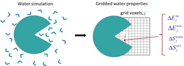
Diagram of a GIST calculation of water properties on a grid (right panel) in and near the binding pocket of a solute (green), based on a molecular dynamics simulation (left panel).
In this communication, we first discuss the algorithms utilized within GIST-cpptraj. Next we outline how to set up and run a GIST-cpptraj analysis of a molecular dynamics trajectory. Then we illustrate how to visualize the results, and how to manipulate the output files with the GISTPP post-processing tool suite. Finally, we analyze the convergence of thermodynamic quantities calculated by GIST.
2. Methods
2.1 Overview of GIST-cpptraj and GISTPP
GIST-cpptraj is a straightforward, command-line tool, included within CPPTRAJ29, which maps out the structural and thermodynamic quantities of water in a user-defined region of interest. This region is partitioned into a high-resolution, three-dimensional (3D) grid (Figure 2), each grid box of which may be viewed as a 3D pixel, or voxel. The grid’s desired size, position, and resolution (i.e. the size of the voxels) are specified via the command line, as detailed in Table 1. Thermodynamic quantities are calculated and mapped to each voxel via the grid based implementation of IST.27 In addition, a variety of structural measures are calculated for the water in each voxel. The thermodynamic and structural properties of water are listed in Table 2.
Figure 2.
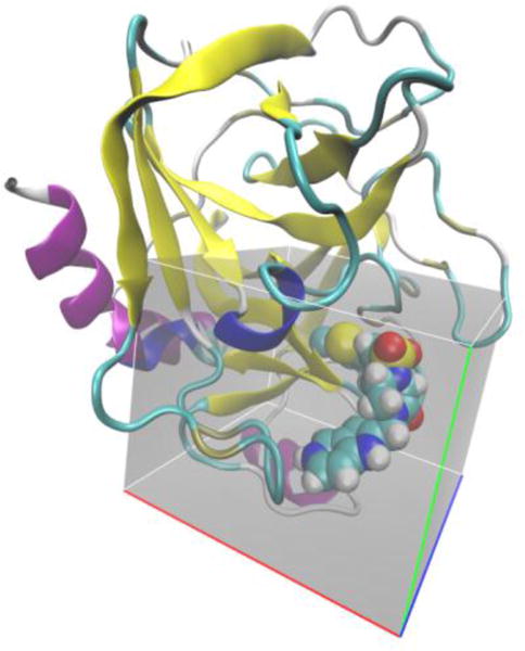
Co-crystal structure of Coagulation Factor Xa (cartoon) with ligand RRR (CPK) from pdb structure 1NFW.34 The region of interest corresponding to the GIST grid is shaded in gray. Individual voxels are not shown.
Table 1.
GIST command options that define the region of interest
| Option | Description | Default Value |
|---|---|---|
| gridcntr | Grid centroid position[a] <x> <y> <z> |
0.0 0.0 0.0 |
| griddim | Grid side length[b] <x> <y> <z> |
40 40 40 |
| gridspacn | Voxel side length[a] | 0.5 |
| refdens | Reference density[c] | 0.0334 |
Quantities in units of angstroms (Å)
Quantity in units of voxel count
Density in molecules per Å3; a list of reference densities for common solvent models can be found in the supplementary information.
Table 2.
Quantities mapped by GIST onto a user-defined volume.
| Quantity | Description | Units |
|---|---|---|
| TStrans | Translational entropy density | kcal/mol/Å3 |
| TSorient | Orientational entropy density | kcal/mol/Å3 |
| TSsix | Total entropy density | kcal/mol/Å3 |
| Eww | Water-water energy density | kcal/mol/Å3 |
| Esw | Solute-water energy density | kcal/mol/Å3 |
| Eij[a] | Voxel pair interaction energy density | kcal/mol |
| Dipole[b] | Mean water dipole density | Debye/Å3 |
| Neighbor count | Mean number of water neighbors[c] | molecules |
| Order[a] | Average tetrahedral order parameter | none |
Optional outputs.
Dipole moments are reported as time-averaged x,y, and z, components, along with the mean magnitude.
Neighbor defined by O-O distance of less than 3.5Å.
By default GIST outputs density weighted thermodynamic quantities from Table 2 in Data Explorer (.dx) file format, enabling visualization with standard graphics packages, such as VMD and PyMol.32,33 Thermodynamic quantities in per water units are not output in the dx file, but are accessible through the space-delimited text output that includes all calculated quantities. A complete list of quantities calculated by GIST can be found in the supplemental information. The GIST post-processing suite of tools, GISTPP, further aids in the analysis of GIST outputs by supporting an array of mathematical and logical operations on .dx files.
2.2 GIST Algorithms
2.2.1 Calculation of hydration entropy terms
The first order entropy calculated by GIST for a voxel k is:
| (1) |
where is the pair correlation function at position and water orientation , is the number density of bulk water, and R is the gas constant. For a voxel , the spatial integral is over the volume of the voxel as indicated by the subscript on the integral symbol. In GIST-cpptraj, is evaluated using two different methods as described below.
Method 1
The first method relies on the approximation that the orientation is independent of the position within each voxel:27,35
| (2) |
This allows the orientational and translational entropy to be evaluated separately within each voxel:
| (3) |
| (4) |
The integrals are estimated using a nearest neighbors approach:36
| (5) |
| (6) |
where is the number of water molecules found in voxel and is Euler’s constant. The quantities are the nearest neighbor estimates for the respective quantities:
| (7) |
and
| (8) |
Here, is the volume of a sphere whose radius is the distance from the current water molecule, , to its nearest neighbor.
| (9) |
| (10) |
The distance in translational space is defined as the Euclidean distance between water oxygens, and the rotational distance is a quaternion distance.37
| (11) |
| (12) |
The NN distances for Methods 1 and 2, below, for waters are calculated from a superset of configurations that includes water coordinates from all stored frames of the simulation. For rotational distances only waters found in the same voxel are used and for translational distances waters within the same and neighboring voxels are used. A voxel is considered to be a neighboring voxel if it shares any of the current voxels vertices, therefore each voxel has 26 neighbors and a voxel combined with all its neighbors form a 3×3×3 cube of voxels.
Method 2
The second method uses an NN approach to directly estimate the six-dimensional integral in Equation 1:38
| (13) |
where the nearest neighbors density, , is:
| (14) |
Here, is the nearest neighbor volume for water , which is the volume of a six dimensional sphere whose radius is the distance between water and its nearest neighbor, in the combined translational and orientational space.
| (15) |
| (16) |
A water’s combined nearest neighbor distance is obtained by considering all waters found within the same and neighboring voxels. Limiting the nearest neighbor search space to this region is computationally efficient and avoids the possibility that position and orientation unit magnitudes can skew the resulting nearest neighbor distance to favor rotations or translations as opposed to their combination.39
2.3 Molecular dynamics simulations
GIST analysis was applied to data from molecular dynamic simulations of cucurbit[7]uril (CB7)40,41 in a box of 1096 TIP3P water molecules, and to coagulation Factor Xa34 in a box of 27381 TIP3P water molecules. The simulations were performed with Amber1430,31 GAFF/AM1-BCC42,43 parameters for cucurbit[7]uril (CB7), Amber14SB44 parameters for Factor Xa, and the TIP3P water model45. GIST mapping was performed with a pre-release version of AmberTools16,30 and all visualizations were conducted using Visual Molecular Dynamics (VMD) 1.9132. The systems were prepared in tleap, minimized with 20,000 steps of the steepest descent algorithm, and then heated to 300 K over 240 ps in the isochoric-isothermal (NVT) ensemble. Each system was then equilibrated for 20 ns in isobaric-isothermal (NPT) conditions at 300K and 1 atm pressure. The production simulation of CB7 was performed for 1 μs and the production simulation of Factor Xa was performed for 150ns. Both production runs were in NVT conditions maintaining a temperature of 300K. The heavy atoms of Factor Xa and CB7 were restrained to the lab frame using harmonic restraints with a force constant of 2.5 kcal/Å2. Temperature was controlled using a Langevin thermostat46 with a collision frequency of γ = 1.0 ps−1. The Berendsen barostat47 with isotropic volume scaling and a coupling constant of 1.0 ps was utilized for pressure regulation. The SHAKE48 algorithm was utilized to constrain the length of bonds to hydrogen at their equilibrium bond length permitting a 2 fs integration time step to be used. Production simulation trajectory coordinate frames were recorded at 1 ps intervals.
3. Results
3.1 Using CPPTRAJ-GIST
GIST requires as input a CPPTRAJ-readable molecular dynamics trajectory file and a corresponding topology file. It is recommended that the simulation be carried out with the atoms of the solute of interest (e.g., a protein) restrained in the lab frame, and that the simulations be run for a minimum of 30 ns,27 with snapshots saved every 3–5 ps for optimal use of nearest neighbor algorithms.38
A GIST study can be broken into three steps:
Step 1. Identify and define the region of interest. The region of interest is a rectangular prism with center (x,y,z) and dimensions (Lx,Ly,Lz) input by the user. Visualization software, such as AutoDockTools,49 can be utilized to determine the grid center and dimensions.
Step 2. Run GIST-cpptraj. The required inputs for running GIST are the MD trajectory and topology files, the coordinates specifying both the dimensions and center of the region of interest and the name of the output file.
Step 3. Analyze GIST results. Visualize and manipulate output.
These steps are detailed below.
Step 1. Identify and define the region of Interest
The location, dimensions and spacing of the 3D grid are defined on the cpptraj command line:
gist gridcntr <xval> <yval>
<zval> griddim <xval> <yval>
<zval> gridspacn <val> out <filename>
Here the gridcntr x, y, and z values define the center of the grid in units of Angstroms (Å). For a protein-binding site a good choice for the center of the grid is at one of the central atoms of a co-crystallized ligand (Figure 2). Note, however, that a common usage is the analysis of water in a binding site in the absence of a ligand. In such simulations the GIST analysis provides information on the structure and thermodynamics of water that is displaced upon ligand binding. In these cases the coordinates of an arbitrary atom in the active site may be convenient, or one may use any preferred method to identify a central position in the binding site. In choosing the grid placement and dimension several docking GUIs may be useful to visualize the region of interest, such as AutoDock Tools.49
The grid is divided into cubic voxels with sides of length gridspacn (Å), and hence volume Vvox=( gridspacn)3, and the number of voxels along each dimension of the box is given by griddim. Smaller voxels provide finer spatial resolution in the GIST maps but require longer simulations to converge. Based on earlier studies the default grid spacing of 0.5 Å provides a reasonable balance of speed, resolution, and convergence of voxel-by-voxel thermodynamic quantities.
Step 2. Run GIST-cpptraj
Since GIST is incorporated into cpptraj, the topology, trajectory files, and GIST command line can all be specified in a simple cpptraj input file. A sample input file, cpptraj.gist.in, follows, with filenames rendered in italics.
parm topology.prmtop
trajin trajectoryfile.mdcrd 1 30000
gist gridcntr 25.0 31.0 30.0 griddim 40 40 40
gridspacn 0.50 out gist.out
go
The first line defines which topology file to use; the second defines the trajectory file and the range of frames to be analyzed, here the first 30,000; the third line defines the center of the grid region to be analyzed and specifies that the region is a cube of dimensions 40×40×40 voxel lengths; the fourth line gives the voxel length of 0.50 Å and defines the name of the output file; and the fifth line tells cpptraj to start the analysis.
The syntax for running cpptraj with input file cpptraj.gist.in is:
cpptraj –i cpptraj.gist.in
Step 3. Analyze GIST results
GIST-cpptraj outputs gridded maps of solvent thermodynamic and structural quantities in dx file format, which can be visualized in most model viewing software, such as VMD and PyMol.32,33 Quantities not printed in dx files by default can be found in the text output and can be converted into dx format, if desired, by GISTPP. When visualized, these maps highlight key features of surface solvation such as high-density regions, or regions where the solvent interacts favorably with the surface or has unfavorable entropy, as illustrated for CB7 in Figure 3. Though in this study we demonstrate the utility of GIST on a host-guest system an in depth application of GIST on a protein-ligand system has been demonstrated previously and is also shown in the AmberTools GIST tutorial.28,35,50
Figure 3.
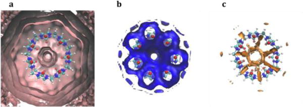
Sample visualizations of GIST output for host molecule CB7. a) Solvation shells around CB7 produced by visualizing gist-gO.dx with cutoff 0.98. b) Favorable solute-water interactions found near the oxygens of CB7, produced by visualizing gist-Esw-dens.dx with cutoff −0.24 (kcal/Å3). c) Unfavorable combined entropy found between the oxygens of CB7, visualized from gist-dTSsix-dens.dx with cutoff −0.18 (kcal/Å3).
3.2 Post-processing results with GISTPP
To aid in GIST analysis we have developed a suite of post-processing tools, GISTPP, which facilitates the manipulation of GIST output files. The GISTPP package provides a comprehensive set of operations that allow end-users to easily manipulate the dx files generated by GIST. Each command specifies an operation, one or two input dx files, an output file, and any options related to the operation:
gistpp –i infile -i2 infile2
–op operation –opt options
–o outfile
A list of the key operations and brief explanations can be found in Table 3. A user manual can be found at ambermd.org.50
Table 3.
Selected GISTPP operations with descriptions
| Operation | Description |
|---|---|
| mult | Multiplies two dx maps together |
| add | Adds two dx maps together |
| sub | Subtracts dx map 2 from dx map 1 |
| div | Divides dx map 1 by dx map 2 |
| filter1 | Create a binary dx[a] map of voxels that are above or below a threshold |
| sum | Integrates all voxel quantities in a given dx map, printing the sum |
| defbp | Create a binary map around a pdb structure by flagging all voxels found within a user defined distance of all heavy atoms. |
| SAS | Creates a dx map of the real solvent accessible surface,19,20 which comprises voxels where the water density is greater than 0.1 of bulk density (g(O) >0.1) and at least one neighbor voxel has water density less than 0.1 of bulk (g(O) <0.1) |
A binary map contains a 1 in each voxel that meets a criterion and a 0 in each voxel that does not.
For example, two dx files can be easily summed together from the command line:
gistpp –i gist-Eww-dens.dx
–i2 gist-Esw-dens.dx –op add
–o Etot.dx
Here, the solute-water energy map and the water-water energy map are summed to obtain a dx map, Etot.dx, of the total water-system energy.
More complex manipulations can be achieved with sequential GISTPP operations. For example, in a previous study, we found that the displacement of high energy and high density water from the Factor Xa binding site was highly correlated to protein-ligand binding affinity.35 To map out such regions, we would first add the water-water energies and the solute-water energies to obtain a total energy map (as shown above). One may then create binary maps, which define voxels with high density and high energy, respectively:
gistpp –i gist-gO.dx –op
filter1 -opt gt1 -opt cutoff1
2 -o Highdens.dx
gistpp -i Etot.dx -op
filter1 –opt gt1 –opt cutoff1
-9.53 -o HighEnergy.dx
Multiplying the binary maps of high density and high energy creates a binary scoring map, which marks only those voxels at both high density and high energy:
gistpp -i Highdens.dx -i2
HighEnergy.dx -op mult -o
ScoringRegions.dx
The scoring regions displaced by a given ligand can then be mapped out by creating a mask of water that is displaced by a given ligand, defined by a PDB file, here RRR.pdb from a congeneric pair study:10
gistpp -i ScoringRegions.dx
-i2 RRR.pdb -op defbp -o
DisplacedRRR.dx
gistpp –i DisplacedRRR.dx –i2
ScoringRegions.dx –op mult –o
ScoringRegionsRRR.dx
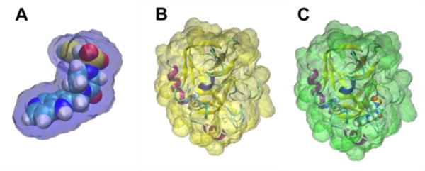
As in our previous study the solvent displacement score for each ligand can then be calculated by finding the number of scoring voxels displaced (Figure 4):
Figure 4.
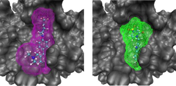
Scoring regions of two ligands from a congeneric pair study of Factor Xa, ligand RRR (left, purple) and 4QC (right, green).10
gistpp -i
ScoringRegionsRRR.dx -op sum
In our previous study,35 we found that the differences in these scores for congeneric pairs of ligands were highly correlated (R2=0.92) with relatively binding affinities from experiment.
3.3 Convergence of entropy
The convergence of the first-order hydration entropy was examined by applying both Method 1 (separated) and Method 2 (combined) to a region within 3 Å of co-crystallized ligand RRR in the Factor Xa binding site, for MD snapshots saved at 1ps intervals. As shown in Figure 5 the translational entropy converges to within 0.002 kcal/mol/water of the final value after 2 ns. The orientational entropy converges to within 0.2 kcal/mol/water of the final value after 2ns; 0.04 kcal/mol/water of the final value after 10ns; and 0.01 kcal/mol/water after 100ns. Convergence of the summed entropy (Figure 5) is thus limited by the orientational component. Interestingly, the combined method (Figure 5), which directly provides the sum of the orientational and translational terms, converges more rapidly than the sum from the separated method, converging to within 0.1 kcal/mol/water by 2 ns, within 0.04 kcal/mol/water by 10ns, and 0.004 kcal/mol/water after 100 ns. The agreement between both methods is excellent, as is evident from Figure 5 and the graph of the difference between the two methods as a function of simulation time (Figure 6). The slight difference between separated and combined nearest neighbor formulations represents the error from smoothing within voxels in the conditionally separated formulation.
Figure 5.
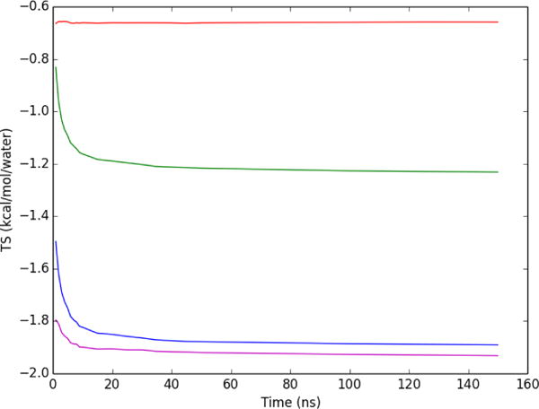
Convergence of per water entropy within a 3 Å volume around the heavy atoms of Factor Xa ligand RRR. Red: translational entropy; green: orientational; blue: sum of translational and orientational; purple: combined six dimensional total entropy (Method 2).
Figure 6.
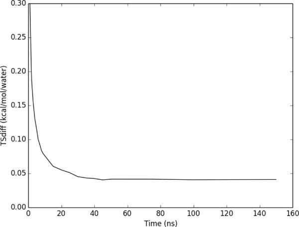
Difference in total first order per water entropy from Method 1 versus Method 2, for a 3 Å volume around the heavy atoms of Factor Xa ligand RRR.
3.4 Convergence of energy
GIST evaluates hydration energy as separate solute-water (Esw) and water-water (Eww) contributions. Here we examine the convergence of their sum (Etot=Esw+Eww), again for the region within 3 Å of the heavy atoms of Factor Xa ligand RRR. As shown in Figure 7 the energy is converged to within 0.1 kcal/mol/water of the final value within 2ns, to within 0.02 kcal/mol/water by 10ns, and 0.004 kcal/mol/water by 100ns respectively.
Figure 7.
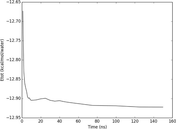
Convergence of Etot, normalized per water molecule, for a region 3 Å around the heavy atoms of Factor Xa ligand RRR.
3.5 End States Analysis
In previous studies we correlated Factor Xa binding affinities with water properties from GIST using a displaced solvent functional.10,35 This analysis relied upon the investigation of the displacement of water from the protein binding site alone and did not include contributions from the solvent reorganization upon binding or from the desolvation of the ligand.
Here we outline how GIST-cpptraj can be used to estimate of a ligand-binding event that includes both the solvent reorganization around the complex and the desolvation of the ligand. In order to do this, three independent MD simulations would be run and analyzed by GIST: the solvated protein-ligand complex, the protein and the ligand. The first step of the analysis would be to identify a region in which the water is energetically and entropically perturbed from bulk values around the solute. This is illustrated in figure 8.
Figure 8.
End states volumes defined around ligand RRR (a, blue), Factor Xa (b, yellow), and the complex formed by these two molecules (c, green). The free energy of solvation defined by these volumes can be used to estimate the free energy of solvation during the binding of ligand RRR.
The next step would be to calculate the perturbation of energy and entropy of the water from bulk in each of these three regions.
Where and are, respectively, the energy and entropy of water found within voxels i the region of interest, is the average number of waters in the perturbed volume, and are the energy and entropy of a single water molecule in the neat solution. The free energy of perturbation would then be:
The change in solvation free energy for the binding process, , would be:
Example GISTPP commands that accomplish this approach for Factor Xa and ligand RRR are provided in the Supplemental Information.
Discussion and Conclusions
The incorporation of GIST calculations into the AMBER CPPTRAJ analysis suite affords a powerful open-source tool for computing and mapping the properties of water at molecular surfaces in high resolution. This is supplemented by the GISTPP post-processing code, which facilitates a wide variety of analyses and visualizations.
Lower resolution implementations of IST using site based approaches have been successful in computer aided-drug design applications, such as describing scoring affinity differences between congeneric pairs of ligands10,51, improving docking and virtual screening, and understanding specificity of binding between members of the same protein family.51–54 These techniques have been applied towards advancing our understanding of the hydrophobic effect55–60 and elucidating where implicit models deviate from explicit and how appropriate corrections to implicit water models can be made.61
GIST’s high-resolution approach has had similar success in correlating binding affinities in Factor Xa and we anticipate a higher resolution picture will afford greater insight in the above and other applications. In particular, the mapping of solvation structure and thermodynamics onto a grid is easily amenable to incorporation into commonly used grid based docking scoring functions. We have also illustrated how GIST can be used in an end states approach that will allow for the straightforward comparisons to other techniques aimed at predicting binding affinities such as free energy perturbation and thermodynamic integration.
Both GIST-cpptraj and GISTPP come with detailed manuals and tutorials. This new toolkit provides users with capabilities to consider surface solvation in basic and applied computational studies, and provides a basis for further method development.
Supplementary Material
Acknowledgments
This publication was made possible in part by grant GM100946 from the National Institutes of Health. Its contents are solely the responsibility of the authors and do not necessarily represent the official views of the NIH.
Footnotes
M.K.G. has an equity interest in and is a cofounder and scientific advisor of VeraChem LLC.
Additional Supporting Information may be found in the online version of this article.
References and Notes
- 1.Wong SE, Lightstone FC. Accounting for water molecules in drug design. Expert Opin Drug Discov. 2010;6:65–74. doi: 10.1517/17460441.2011.534452. [DOI] [PubMed] [Google Scholar]
- 2.Abel R, Wang L, Friesner RA, Berne BJ. A Displaced-Solvent Functional Analysis of Model Hydrophobic Enclosures. J Chem Theory Comput. 2010;6:2924–2934. doi: 10.1021/ct100215c. [DOI] [PMC free article] [PubMed] [Google Scholar]
- 3.Bissantz C, Kuhn B, Stahl M. A Medicinal Chemist’s Guide to Molecular Interactions. J Med Chem. 2010;53:5061–5084. doi: 10.1021/jm100112j. [DOI] [PMC free article] [PubMed] [Google Scholar]
- 4.Riniker S, et al. Free enthalpies of replacing water molecules in protein binding pockets. J Comput Aided Mol Des. 2012;26:1293–1309. doi: 10.1007/s10822-012-9620-8. [DOI] [PubMed] [Google Scholar]
- 5.Poornima CS, Dean PM. Hydration in drug design. 1. Multiple hydrogen-bonding features of water molecules in mediating protein-ligand interactions. J Comput Aided Mol Des. 1995;9:500–512. doi: 10.1007/BF00124321. [DOI] [PubMed] [Google Scholar]
- 6.García-Sosa AT, Firth-Clark S, Mancera RL. Including Tightly-Bound Water Molecules in de Novo Drug Design. Exemplification through the in Silico Generation of Poly(ADP-ribose)polymerase Ligands. J Chem Inf Model. 2005;45:624–633. doi: 10.1021/ci049694b. [DOI] [PubMed] [Google Scholar]
- 7.Ladbury JE. Just add water! The effect of water on the specificity of protein-ligand binding sites and its potential application to drug design. Chem Biol. 1996;3:973–980. doi: 10.1016/s1074-5521(96)90164-7. [DOI] [PubMed] [Google Scholar]
- 8.Hummer G. Molecular binding: Under water’s influence. Nat Chem. 2010;2:906–907. doi: 10.1038/nchem.885. [DOI] [PMC free article] [PubMed] [Google Scholar]
- 9.Rl M. Molecular modeling of hydration in drug design. Curr Opin Drug Discov Devel. 2007;10:275–280. [PubMed] [Google Scholar]
- 10.Abel R, Young T, Farid R, Berne BJ, Friesner RA. Role of the Active-Site Solvent in the Thermodynamics of Factor Xa Ligand Binding. J Am Chem Soc. 2008;130:2817–2831. doi: 10.1021/ja0771033. [DOI] [PMC free article] [PubMed] [Google Scholar]
- 11.Li Z, Lazaridis T. Thermodynamic Contributions of the Ordered Water Molecule in HIV-1 Protease. J Am Chem Soc. 2003;125:6636–6637. doi: 10.1021/ja0299203. [DOI] [PubMed] [Google Scholar]
- 12.Li Z, Lazaridis T. Thermodynamics of Buried Water Clusters at a Protein−Ligand Binding Interface. J Phys Chem B. 2006;110:1464–1475. doi: 10.1021/jp056020a. [DOI] [PubMed] [Google Scholar]
- 13.Baron R, Setny P, Andrew McCammon J. Water in Cavity−Ligand Recognition. J Am Chem Soc. 2010;132:12091–12097. doi: 10.1021/ja1050082. [DOI] [PMC free article] [PubMed] [Google Scholar]
- 14.Young T, Abel R, Kim B, Berne BJ, Friesner RA. Motifs for molecular recognition exploiting hydrophobic enclosure in protein–ligand binding. Proc Natl Acad Sci. 2007;104:808–813. doi: 10.1073/pnas.0610202104. [DOI] [PMC free article] [PubMed] [Google Scholar]
- 15.Imai T, Hiraoka R, Kovalenko A, Hirata F. Water Molecules in a Protein Cavity Detected by a Statistical−Mechanical Theory. J Am Chem Soc. 2005;127:15334–15335. doi: 10.1021/ja054434b. [DOI] [PubMed] [Google Scholar]
- 16.Baroni M, Cruciani G, Sciabola S, Perruccio F, Mason JS. A Common Reference Framework for Analyzing/Comparing Proteins and Ligands. Fingerprints for Ligands And Proteins (FLAP): Theory and Application. J Chem Inf Model. 2007;47:279–294. doi: 10.1021/ci600253e. [DOI] [PubMed] [Google Scholar]
- 17.Molecular Discovery Ltd. Pinner, UK. FLAP/WaterFLAP. 2013 [Google Scholar]
- 18.Bayden AS, Moustakas DT, Joseph-McCarthy D, Lamb ML. Evaluating Free Energies of Binding and Conservation of Crystallographic Waters Using SZMAP. J Chem Inf Model. 2015 doi: 10.1021/ci500746d. [DOI] [PubMed] [Google Scholar]
- 19.Velez-Vega C, McKay DJJ, Aravamuthan V, Pearlstein R, Duca JS. Time-Averaged Distributions of Solute and Solvent Motions: Exploring Proton Wires of GFP and PfM2DH. J Chem Inf Model. 2014;54:3344–3361. doi: 10.1021/ci500571h. [DOI] [PubMed] [Google Scholar]
- 20.Velez-Vega C, et al. Estimation of Solvation Entropy and Enthalpy via Analysis of Water Oxygen–Hydrogen Correlations. J Chem Theory Comput. 2015;11:5090–5102. doi: 10.1021/acs.jctc.5b00439. [DOI] [PMC free article] [PubMed] [Google Scholar]
- 21.Cui G, Swails JM, Manas ES. SPAM: A Simple Approach for Profiling Bound Water Molecules. J Chem Theory Comput. 2013;9:5539–5549. doi: 10.1021/ct400711g. [DOI] [PubMed] [Google Scholar]
- 22.Hu B, Lill MA. WATsite: Hydration site prediction program with PyMOL interface. J Comput Chem. 2014;35:1255–1260. doi: 10.1002/jcc.23616. [DOI] [PMC free article] [PubMed] [Google Scholar]
- 23.Zheng Li TL. Computing the Thermodynamic Contributions of Interfacial Water. Methods Mol Biol Clifton NJ. 2012;819:393–404. doi: 10.1007/978-1-61779-465-0_24. [DOI] [PubMed] [Google Scholar]
- 24.Michel J, Tirado-Rives J, Jorgensen WL. Prediction of the Water Content in Protein Binding Sites. J Phys Chem B. 2009;113:13337–13346. doi: 10.1021/jp9047456. [DOI] [PMC free article] [PubMed] [Google Scholar]
- 25.Fraser CM, Fernández A, Scott LR, Fraser CM. WRAPPA: A Screening Tool for Candidate Dehydron Identification [Google Scholar]
- 26.López ED et al. WATCLUST: a tool for improving the design of drugs based on protein-water interactions. Bioinformatics. 2015 doi: 10.1093/bioinformatics/btv411. btv411. [DOI] [PubMed] [Google Scholar]
- 27.Nguyen CN, Young TK, Gilson MK. Grid inhomogeneous solvation theory: Hydration structure and thermodynamics of the miniature receptor cucurbit[7]uril. J Chem Phys. 2012;137:44101. doi: 10.1063/1.4733951. [DOI] [PMC free article] [PubMed] [Google Scholar]
- 28.Nguyen C, Gilson MK, Young T. Structure and Thermodynamics of Molecular Hydration via Grid Inhomogeneous Solvation Theory. ArXiv11084876 Phys Q-Bio. 2011 doi: 10.1063/1.4733951. [DOI] [PMC free article] [PubMed] [Google Scholar]
- 29.Roe DR, Cheatham TE. PTRAJ and CPPTRAJ: Software for Processing and Analysis of Molecular Dynamics Trajectory Data. J Chem Theory Comput. 2013;9:3084–3095. doi: 10.1021/ct400341p. [DOI] [PubMed] [Google Scholar]
- 30.Case DA, Berryman JT, Betz RM, Cerutti DS, Cheatham TE, III, Darden TA, Duke RE, Giese TJ, Gohlke H, Goetz AW, Homeyer N, Izadi S, Janowski P, Kaus J, Kovalenko A, Lee TS, LeGrand S, Li P, Luchko T, Luo R, Madej B, Merz KM, Monard G, Needham P, Nguyen H, Nguyen HT, Omelyan I, Onufriev A, Roe DR, Roitberg A, Salomon-Ferrer R, Simmerling CL, Smith W, Swails J, Walker RC, Wang J, Wolf RM, Wu X, York DM, Kollman PA. Amber 2015. Univ Calif San Fransisco. 2015 [Google Scholar]
- 31.Salomon-Ferrer R, Case DA, Walker RC. An overview of the Amber biomolecular simulation package. Wiley Interdiscip Rev Comput Mol Sci. 2013;3:198–210. [Google Scholar]
- 32.Humphrey W, Dalke A, Schulten K. VMD: Visual molecular dynamics. J Mol Graph. 1996;14:33–38. doi: 10.1016/0263-7855(96)00018-5. [DOI] [PubMed] [Google Scholar]
- 33.Delano W. The PyMOL Molecular Graphics System. 2002 [Google Scholar]
- 34.Maignan S, et al. Molecular Structures of Human Factor Xa Complexed with Ketopiperazine Inhibitors: Preference for a Neutral Group in the S1 Pocket. J Med Chem. 2003;46:685–690. doi: 10.1021/jm0203837. [DOI] [PubMed] [Google Scholar]
- 35.Nguyen CN, Cruz A, Gilson MK, Kurtzman T. Thermodynamics of Water in an Enzyme Active Site: Grid-Based Hydration Analysis of Coagulation Factor Xa. J Chem Theory Comput. 2014;10:2769–2780. doi: 10.1021/ct401110x. [DOI] [PMC free article] [PubMed] [Google Scholar]
- 36.Harshinder Singh VH. Nearest Neighbor Estimates of Entropy. Am J Math Manag Sci. 2003;23 [Google Scholar]
- 37.Huggins DJ. Comparing distance metrics for rotation using the k-nearest neighbors algorithm for entropy estimation. J Comput Chem. 2014;35:377–385. doi: 10.1002/jcc.23504. [DOI] [PMC free article] [PubMed] [Google Scholar]
- 38.Huggins DJ. Estimating Translational and Orientational Entropies Using the k-Nearest Neighbors Algorithm. J Chem Theory Comput. 2014;10:3617–3625. doi: 10.1021/ct500415g. [DOI] [PubMed] [Google Scholar]
- 39.Fogolari F, et al. Accurate Estimation of the Entropy of Rotation–Translation Probability Distributions. J Chem Theory Comput. 2016;12:1–8. doi: 10.1021/acs.jctc.5b00731. [DOI] [PubMed] [Google Scholar]
- 40.Kim J, et al. New Cucurbituril Homologues: Syntheses, Isolation, Characterization, and X-ray Crystal Structures of Cucurbit[n]uril (n = 5, 7, and 8) J Am Chem Soc. 2000;122:540–541. [Google Scholar]
- 41.Jeon WS, et al. Complexation of Ferrocene Derivatives by the Cucurbit[7]uril Host: A Comparative Study of the Cucurbituril and Cyclodextrin Host Families. J Am Chem Soc. 2005;127:12984–12989. doi: 10.1021/ja052912c. [DOI] [PubMed] [Google Scholar]
- 42.Wang J, Wolf RM, Caldwell JW, Kollman PA, Case DA. Development and testing of a general amber force field. J Comput Chem. 2004;25:1157–1174. doi: 10.1002/jcc.20035. [DOI] [PubMed] [Google Scholar]
- 43.Jakalian A, Jack DB, Bayly CI. Fast, efficient generation of high-quality atomic charges. AM1-BCC model: II. Parameterization and validation. J Comput Chem. 2002;23:1623–1641. doi: 10.1002/jcc.10128. [DOI] [PubMed] [Google Scholar]
- 44.Maier JA, et al. ff14SB: Improving the Accuracy of Protein Side Chain and Backbone Parameters from ff99SB. J Chem Theory Comput. 2015 doi: 10.1021/acs.jctc.5b00255. [DOI] [PMC free article] [PubMed] [Google Scholar]
- 45.Jorgensen WL, Chandrasekhar J, Madura JD, Impey RW, Klein ML. Comparison of simple potential functions for simulating liquid water. J Chem Phys. 1983;79:926–935. [Google Scholar]
- 46.Pastor RW, Brooks BR, Szabo A. An analysis of the accuracy of Langevin and molecular dynamics algorithms. Mol Phys. 1988;65:1409–1419. [Google Scholar]
- 47.Allen Mike P, Tildesley Dominic J. Computer Simulation of Liquids. Oxford University Press; 1989. [Google Scholar]
- 48.Ryckaert JP, Ciccotti G, Berendsen HJC. Numerical integration of the cartesian equations of motion of a system with constraints: molecular dynamics of n-alkanes. J Comput Phys. 1977;23:327–341. [Google Scholar]
- 49.Morris GM, et al. AutoDock4 and AutoDockTools4: Automated docking with selective receptor flexibility. J Comput Chem. 2009;30:2785–2791. doi: 10.1002/jcc.21256. [DOI] [PMC free article] [PubMed] [Google Scholar]
- 50.AMBER Advanced Tutorial 25 – Grid Inhomogeneous Solvent Theory (GIST) Example: Introduction. Available at: http://ambermd.org/tutorials/advanced/tutorial25/. (Accessed: 4th January 2016)
- 51.Robert Abel NKS. Contribution of Explicit Solvent Effects to the Binding Affinity of Small-Molecule Inhibitors in Blood Coagulation Factor Serine Proteases. ChemMedChem. 2011;6:1049–66. doi: 10.1002/cmdc.201000533. [DOI] [PubMed] [Google Scholar]
- 52.Shah F, et al. Computer-Aided Drug Design of Falcipain Inhibitors: Virtual Screening, Structure–Activity Relationships, Hydration Site Thermodynamics, and Reactivity Analysis. J Chem Inf Model. 2012;52:696–710. doi: 10.1021/ci2005516. [DOI] [PubMed] [Google Scholar]
- 53.Pearlstein RA, Sherman W, Abel R. Contributions of water transfer energy to protein-ligand association and dissociation barriers: Watermap analysis of a series of p38α MAP kinase inhibitors. Proteins Struct Funct Bioinforma. 2013;81:1509–1526. doi: 10.1002/prot.24276. [DOI] [PubMed] [Google Scholar]
- 54.Beuming T, et al. Thermodynamic analysis of water molecules at the surface of proteins and applications to binding site prediction and characterization. Proteins Struct Funct Bioinforma. 2012;80:871–883. doi: 10.1002/prot.23244. [DOI] [PubMed] [Google Scholar]
- 55.Lazaridis T. Solvent Size vs Cohesive Energy as the Origin of Hydrophobicity. Acc Chem Res. 2001;34:931–937. doi: 10.1021/ar010058y. [DOI] [PubMed] [Google Scholar]
- 56.Lazaridis T, Paulaitis ME. Entropy of hydrophobic hydration: a new statistical mechanical formulation. J Phys Chem. 1992;96:3847–3855. [Google Scholar]
- 57.Fox JM, et al. Interactions between Hofmeister Anions and the Binding Pocket of a Protein. J Am Chem Soc. 2015;137:3859–3866. doi: 10.1021/jacs.5b00187. [DOI] [PMC free article] [PubMed] [Google Scholar]
- 58.Snyder PW, et al. Mechanism of the hydrophobic effect in the biomolecular recognition of arylsulfonamides by carbonic anhydrase. Proc Natl Acad Sci. 2011;108:17889–17894. doi: 10.1073/pnas.1114107108. [DOI] [PMC free article] [PubMed] [Google Scholar]
- 59.Lockett MR, et al. The Binding of Benzoarylsulfonamide Ligands to Human Carbonic Anhydrase is Insensitive to Formal Fluorination of the Ligand. Angew Chem Int Ed. 2013;52:7714–7717. doi: 10.1002/anie.201301813. [DOI] [PubMed] [Google Scholar]
- 60.Breiten B, et al. Water Networks Contribute to Enthalpy/Entropy Compensation in Protein–Ligand Binding. J Am Chem Soc. 2013;135:15579–15584. doi: 10.1021/ja4075776. [DOI] [PubMed] [Google Scholar]
- 61.Wickstrom L, et al. Parameterization of an effective potential for protein–ligand binding from host–guest affinity data. J Mol Recognit JMR. 2016;29:10–21. doi: 10.1002/jmr.2489. [DOI] [PMC free article] [PubMed] [Google Scholar]
Associated Data
This section collects any data citations, data availability statements, or supplementary materials included in this article.