Realistic models of apparent dynamic changes in resting‐state connectivity in somatosensory cortex

Abstract

Variations over time in resting‐state correlations in blood oxygenation level‐dependent (BOLD) signals from different cortical areas may indicate changes in brain functional connectivity. However, apparent variations over time may also arise from stationary signals when the sample duration is finite. Recently, a vector autoregressive (VAR) null model has been proposed to simulate real functional magnetic resonance imaging (fMRI) data, which provides a robust stationary model for identifying possible temporal dynamic changes in functional connectivity. In this work, we propose a simpler model that uses a filtered stationary dataset. The filtered stationary model generates statistically stationary time series from random data with a single prescribed correlation coefficient that is calculated as the average over the entire time series. In addition, we propose a dynamic model, which is better able to replicate real fMRI connectivity, estimated from monkey brain studies, than the two stationary models. We compare simulated results using these three models with the behavior of primary somatosensory cortex (S1) networks in anesthetized squirrel monkeys at high field (9.4 T), using a sliding window correlation analysis. We found that at short window sizes, both stationary models reproduced the distribution of correlations of real signals well, but at longer window sizes, a dynamic model reproduced the distribution of correlations of real signals better than the stationary models. While stationary models replicate several features of real data, a close representation of the behavior of resting‐state data acquired from somatosensory cortex of non‐human primates is obtained only when a dynamic correlation is introduced, suggesting dynamic variations in connectivity are real. Hum Brain Mapp 37:3897–3910, 2016. © 2016 Wiley Periodicals, Inc.

INTRODUCTION

Low frequency fluctuations in blood oxygenation level‐dependent (BOLD) functional magnetic resonance imaging (fMRI) signals may occur spontaneously in functionally related areas of the cortex in the absence of any specific task [Biswal et al., 1995]. Biswal et al. [1995] first reported the correlation in fMRI signal fluctuations between the left and right motor cortices when the brain was in a resting state. Functionally related brain regions can be identified using their synchronous slow fluctuations in signal intensity [Cordes et al., 2000]. Subsequent studies have identified several consistent resting‐state networks, including motor, auditory, visual, attention, and default mode [Damoiseaux et al., 2006; Greicius et al., 2003].

Various techniques have been used to derive functional connectivity to reveal functionally related brain regions [Beckmann et al., 2005; Power et al., 2011; Yeo et al., 2011]. For example, seed‐based region‐of‐interest (ROI) analyses, in which the time series of an ROI is used as a regressor to identify regions of similar temporal behavior elsewhere in the brain [Biswal et al., 1995; Lowe et al., 1998], quantify the relationship between two ROIs as a single correlation coefficient that is calculated from the entire scan duration. Possible temporal variations in this value are not captured by this approach. Another common technique is spatial independent component analysis [Beckmann et al., 2005; McKeown et al., 1998], a model‐free approach for identifying spatial regions with temporally coordinated activity. It decomposes the fMRI data into a prescribed number of components with maximal spatial independence. While this strategy avoids the inconvenience and possible inaccuracy from selecting specific seed regions, it again does not incorporate possible changes in inter‐regional interactions over time. Other methods for characterizing resting‐state networks include clustering [Mezer et al., 2009; Yeo et al., 2011], phase relationships [Sun et al., 2005], and graph theory [Achard et al., 2006; Dosenbach et al., 2007].

Most fMRI studies in the past have assumed that the correlations between brain regions are constant throughout the time series of the entire scan in resting‐state experiments [Fox et al., 2005; Fransson, 2005; Greicius et al., 2003]. More recently, there has been an increasing interest in the detection and characterization of possible dynamic changes in functional connectivity [Allen et al., 2014; Chang and Glover, 2010; Hutchison et al., 2013a, 2013b]. Variations in the degree of coupling between different networks would seem to be a plausible feature of neural systems, and the nature of temporal changes in such couplings could be an important aspect of brain function. However, the unambiguous detection and quantification of dynamic changes in correlations are not trivial, and are similar to the well‐known difficulties in classifying data as statistically stationary or non‐stationary. Whether observed dynamic changes in correlations between distinct brain regions over time show significantly greater variability than would be expected if the underlying correlation coefficient between the two signals were stationary (time‐invariant) is a crucial issue. Currently, there is no consensus on which analysis technique is the most effective at characterizing such temporal variations in resting‐state fMRI signals. The most commonly used strategy for analyzing dynamic changes in resting‐state functional connectivity has been a sliding window correlation approach [Allen et al., 2014; Chang and Glover, 2010; Handwerker et al., 2012; Hutchison et al., 2013a, 2013b; Jones et al., 2012; Sakoglu et al., 2010], which is intended to identify pairwise variations in inter‐regional time courses. The limitations of this approach are clear and further discussed below. Other methods, for example, the PsychoPhysiological Interactions [PPI; Friston et al., 1997] method studies the dynamical feature of functional connectivity under the assumption that the timing of the various contexts or state changes is known. However, it is often difficult to identify or specify the timing and duration of the psychological processes being studied a priori. Cribben et al. introduced a Dynamic Connectivity Regression technique, which is a data‐driven method for detecting functional connectivity change points between brain regions where the number of change points and their locations are unknown in advance [Cribben et al., 2012]. While this strategy avoids the assumption of knowing state changes in advance, it does not estimate details of the dynamic correlation between the brain regions. Various efforts have also been made to replicate real resting‐state fMRI data using simulated time series, most notably the vector autoregressive (VAR) null model [Chang and Glover, 2010; Cribben et al., 2013; Shah et al., 2012; Zalesky et al., 2014] which avoids possible confounds from physiological noise or other sources of artifact.

The purpose of this study was to evaluate whether correlations in real fMRI data are stationary, and to investigate the existence of dynamic correlations. Our motivation was to simulate the behavior of the temporal correlations between different sub‐regions in S1 cortex of monkey brain over an 18‐min resting‐state scanning session. We first used a VAR null model and then developed a simpler model that uses a filtered stationary simulation dataset, whose behavior could then be compared to real resting‐state fMRI data. The filtered stationary model generates statistically stationary time series from random data with a single prescribed correlation coefficient that is calculated as the average over the entire time series. We then further modified the model to account for the dynamic features in connectivity, and used a variant of the Kolmogorov–Smirnov (K‐S) statistic to quantitatively compare all simulated results to the behavior of real networks. We used a very well characterized network for dynamic functional connectivity studies. Our experimental data were obtained from small regions in the somatosensory (S1) networks in anesthetized squirrel monkeys at high field strength (9.4 T) [Chen et al., 2011; Friedman et al., 2011; Wang et al., 2013; Zhang et al. 2007]. The hand–face region within the S1 cortex of the squirrel monkey has been previously well mapped with functional imaging, electrophysiological and anatomical methods, and the orderly topographic map of the hand region is characterized by a lateral to medial representation of individual digits in three sub‐regions of areas 3a, 3b, and 1 [Chen et al., 2011].

MATERIALS AND METHODS

Animal Preparation

Three squirrel monkeys (three sessions each) were pre‐anesthetized with ketamine hydrochloride (10 mg/kg)/atropine (0.05 mg/kg) and then anesthetized with 0.5–1.5% of isoflurane to maintain a stable physiological condition for MRI scans. Although the actual level may vary across animals, we typically maintained anesthesia under a light stable level around 0.7–0.8% during our functional data acquisition. The anesthetized animals were intubated and artificially ventilated. After intubation, each animal was placed in a custom‐designed MR cradle with its head secured using ear bars and an eye bar. Lactated Ringer's solution was infused intravenously (2–3 mL/h/kg) to prevent dehydration during the course of the study. Arterial blood oxygen saturation and heart rate (Nonin, Plymouth, MN), electrocardiogram, end‐tidal CO₂ (ET‐CO₂; 22–26 mm Hg; Surgivet, Waukesha, WI), and respiration (SA Instruments, Stony Brook, NY) were externally monitored and maintained. Temperature (37.5–38.5°C) was monitored (SA Instruments) and maintained via a circulating water blanket (Gaymar Industries, Orchard Park, NY). Real‐time monitoring was maintained from the time of induction of anesthesia until full recovery. Detailed procedures have been described in a previous publication [Chen et al., 2007]. All procedures were in compliance with and approved by the Institutional Animal Care and Use Committee of Vanderbilt University.

fMRI Data Acquisition and Preprocessing

MRI imaging was performed on a 9.4 T 21 cm bore Varian Inova magnet (Varian Medical Systems, Palo Alto, CA), using a 3‐cm surface transmit–receive coil secured over the sensory cortex. Scout images obtained using a fast gradient‐echo sequence were used to define a volume covering primary somatosensory cortex in which static magnetic field homogeneity was optimized, and to plan four oblique slices for structural and functional imaging (Fig. 1, only the top slice shown). T2*‐weighted gradient‐echo structural images [repetition time (TR), 200 ms; echo time (TE) =16 ms, four slices, 512 × 512 matrix; 68 × 68 × 2000 µm³ resolution; number of excitations = 6] were acquired to identify venous structures on the cortical surface used to help locate S1, and as structural features for coregistration of fMRI images. fMRI data were acquired from the same slice. For each monkey, three runs of 720 continuous functional gradient echo‐planar image (EPI) functional volumes (TE =16 ms; 64 × 64 matrix; 547 × 547 × 2000 µm³ resolution) were acquired. Acquisition time of each run was 18 min, and the TR was 1.5 s. Images were reconstructed on the MR console (Varian VnmrJ) and imported into Matlab (Mathworks, Natick, MA) for analysis. The raw echo‐planar images were spatially smoothed with a 3 × 3‐voxel Gaussian window with a standard deviation of 312 µm, and then interpolated to a 256 × 256 matrix for overlay on anatomical images. Time courses were drift corrected using a linear model fitted to each time course and temporally smoothed with a low‐pass filter.

Figure 1.

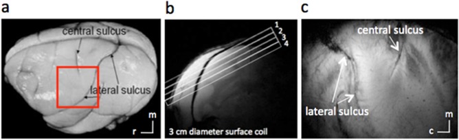
Anatomic images for studying S1. (a) Major landmarks (such as central and lateral sulci) used to identify S1 are visible on squirrel monkey brain. The red box indicates the location of ROIs. (b) A high‐resolution coronal image is collected to locate somatosensory cortices and to guide placement of an oblique slice parallel to S1 (locations indicated by rectangles, overlaid, or coronal scout image). This oblique orientation was used for both high‐resolution anatomical and functional imaging.(c) In an image acquired with T2* weighting, sulci and vascular structures appear dark. Both central and lateral sulci are readily identified in the most superficial slice. c, caudal; m, medial; r, rostral. [Color figure can be viewed at http://wileyonlinelibrary.com]

Identification of ROI Seeds

Specific ROI seeds were identified according to the vibrotactile stimulus evoked activation maps, which were obtained by separate fMRI runs within the same imaging session. A stimulus‐evoked fMRI activation map was used to locate the finger pad regions in areas 3a, 3b, and 1 (see Fig. 2). The fingers were secured by gluing small pegs to the fingernails and fixing these pegs firmly in plasticine, leaving the glabrous surfaces available for vibrotactile stimulation by a rounded plastic probe (2 mm diameter) connected to a piezoelectric device (Noliac, Kvistgaard, Denmark). Piezos were driven by Grass S48 square wave stimulators (Grass‐Telefactor, West Warwick, RI) at a rate of 8 Hz with 30 ms pulse duration. Stimulation was applied in blocks of 30 s on and then 30 s off. The timing of the presentation of stimuli was externally controlled by the MR scanner. The correlation of each functional EPI time course to a reference waveform was calculated and activation maps (Fig. 2) were generated by identifying voxels whose correlation with the reference waveform was significant at least at P ≤ 10⁻⁴ (uncorrected for multiple comparisons). Voxels with the highest P values were chosen as seeds (small blue boxes in Fig. 2), from which filtered resting‐state fMRI time courses were extracted for the dynamic functional connectivity analysis.

Figure 2.

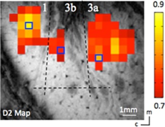
Localization of digit regions with fMRI mapping in the S1 cortex of squirrel monkeys. One case is shown here. BOLD activation in response to vibrotactile stimulation of the D2 tip. Activated voxels are observed in areas 3a, 3b, and 1. Correlation maps were thresholded at r > 0.7, with a peak correlation value of 0.9. Dotted black line indicates approximate inter‐area borders. Blue boxes show the seed voxels. Scale bar, 1 mm. c, caudal; m, medial. [Color figure can be viewed at http://wileyonlinelibrary.com]

Vector Autoregressive Null Model

The VAR model used to capture linear interdependencies among multiple time series [Hacker and Hatemi, 2005] is described in the following text [Chang and Glover, 2010]:

Let x and y represent the BOLD signal time series from two different ROIs in S1 cortex. We first fit a (stationary) VAR model to x and y:

$$\{\begin{array}{c}x(t)={\displaystyle \sum _{i=1}^p{a}_i^{x}x(t-i)}+{\displaystyle \sum _{i=1}^p{b}_i^{x}y(t-i)+{\varepsilon }^x(t)}\\ y(t)={\displaystyle \sum _{i=1}^p{a}_i^{y}x(t-i)}+{\displaystyle \sum _{i=1}^p{b}_i^{y}y(t-i)+{\varepsilon }^y(t)}\end{array},$$ (1)

where the optimal model order p (p = 9) is chosen according to the Bayesian information criterion (BIC) score, and t is a time index. Coefficients of the VAR model are estimated using least squares. Next, we generate 1,000 bootstrap time series pairs having the same VAR coefficients (i.e., same stationary relationship) as Eq. (1).

Filtered Stationary (FTS) Null Model

Let x_c represent the common signal in the BOLD signal time series x ₁ and x ₂ from two different ROIs in S1 cortex. x_c, w ₁, and w ₂ are stationary Gaussian zero‐mean signals, low‐pass filtered to contain frequencies only in the BOLD range 0.01–0.1 Hz. Each time course is independent, and contains 720 time points with an effective TR = 1.5 s.

$$\{\begin{array}{c}{x}_1(t)=x_c(t)+b*w_1(t)\hfill \\ x_2(t)=x_c(t)+b*w_2(t)\hfill \\ \text{corr}(x_1(t),x_2(t))=r(\text{constant})\\ b^2=\frac{1}{\left|r\right|}-1\hfill \end{array},$$ (2)

where the coefficient b is determined by the correlation coefficient between the BOLD signal time series from two different ROIs, and t is a time index. Then we generate 1,000 trials based on Eq. (2).

Sliding Window Correlation Analysis

A sliding window correlation analysis is a method for capturing variations in inter‐regional synchrony [Hutchison et al., 2013a, 2013b], and is commonly used to investigate dynamic changes in correlations between fMRI time series. In this approach, a time window of fixed length is selected, and data points within that window are used to calculate correlation coefficients between two time series (x and y), which are defined as r(t) = corr (x^{t + s−1,} y^{t + s−1}), where s is the window size, x^{t + s−1} and y^{t + s−1} represent the parts of the time series from time t to t + s − 1, and corr () denotes computation of the Pearson's correlation coefficient. The window is then shifted in time by a fixed number of data points (ranging from a single data point to the length of a window) that defines the amount of overlap between successive windows. The correlations between the time series derived from sub‐regions 3a, 3b, and 1 of S1 cortex in monkeys were calculated for window sizes of 30s (20 volumes), 45s (30 volumes), 90s (60 volumes), 135s (90 volumes), 180s (120 volumes), 225s (150 volumes), and 270s (180 volumes). The window was then shifted in time by 1.5s (1 volume) along the entire time series and the correlation coefficient was recalculated. Figure 3 shows an example of the sliding window correlation analysis comparing real fMRI data and two stationary (the VAR and the filtered stationary) null model simulations, with a window size of 60s. This procedure was repeated for all possible window positions within the 720 images of a run. The pairwise sliding window correlations between each of the three sub‐regions were calculated for all animals and all scans.

Figure 3.

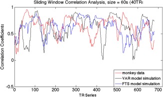
Example of the sliding window correlation analysis comparing real fMRI data and two stationary (the VAR and the filtered stationary) null models, with a window size of 60s (40 TRs). [Color figure can be viewed at http://wileyonlinelibrary.com]

Underlying Dynamic Null Model

To obtain better approximations than stationary null models of the potential dynamic behavior of real data, we first computed correlation coefficients between two ROIs in monkey brain using a sliding window technique with a window size of 135s, and performed a median filtering of the time course of the correlation coefficient. Each time point then contained the median value in the neighborhood of 20 values around the corresponding pixel in the input image. We then fit the smoothed underlying correlations with a sum of 4 sine functions (an example is illustrated in Fig. 4). We define this function as an underlying non‐stationary correlation function r(t) between these two ROIs. Next, we generated 1,000 trials based on Eq. (3). This dynamic simulation can then be compared to the real data.

$$\{\begin{array}{c}{x}_1(t)=x_c(t)+b*w_1(t)\hfill \\ x_2(t)=x_c(t)+b*w_2(t)\hfill \\ \text{corr}(x_1(t),x_2(t))=r(t)(\text{non}‐\text{stationary})\\ b{(t)}^2=\frac{1}{|r(t)|}-1\hfill \end{array},$$ (3)

Figure 4.

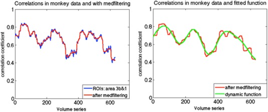
(a) Example of correlations between sub‐regions area 3b and 1 in one monkey using the sliding window technique with a window size of 135s, along with a median filtering smoothing. (b) Example of fitted underlying correlation function: a sum of sines, the number of terms is 4. [Color figure can be viewed at http://wileyonlinelibrary.com]

A Two‐Sample Kolmogorov–Smirnov Statistic

Above, we have described the methods to compute the VAR, filtered stationary, and underlying dynamic null model of a given pair of time series. In this section, we quantify the resemblance of the temporal variations in the correlations between the real and simulated data. We perform a sliding window analysis at one window size and construct the empirical cumulative distribution function (ECDF) for each pair of time series. A two‐sample Kolmogorov–Smirnov (K‐S) statistic [Chakravart, 1967] may be used to evaluate whether two samples come from the same population with a specific distribution, based on measurements of the distance between two ECDFs. It is sensitive to differences in both the location and shape of the ECDFs of the two samples [Marsaglia et al., 2003; Stephens, 1974]. Therefore, lower K‐S values between real and simulated data suggest increased accuracy of the model in representing the nature of the real data.

Centering z‐Scores

As the sampling distribution of Pearson's r is not normally distributed, correlation values were converted to z‐scores using Fisher's z transform. The K‐S results are affected by two main factors, one is the location, and the other is the shape of distribution. To compare distribution shapes, z‐scores were centered by subtracting their mean values (Fig. 5).

Figure 5.

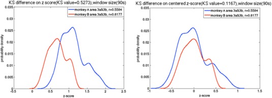
Example of the probability density function of the z‐score between sub‐regions pair 3a–3b of S1 in two different monkeys before and after centering the z‐score. [Color figure can be viewed at http://wileyonlinelibrary.com]

Illustrative Example of Stationary Models

All sub‐region ROI pairs from nine sessions in three monkeys were quantified. Figures 3 and 6 illustrate examples of the results of the sliding window correlation analysis and correlation distributions of actual data and simulated time series, respectively. The correlation coefficient between sub‐regions 3b and 1 in S1 cortex of one randomly selected squirrel monkey calculated from the time series of the entire 20‐min scan is 0.8144. To simulate fMRI data using the filtered stationary null model, only this correlation coefficient is required. We thus generated two time‐series of random signals with correlation coefficient of 0.8144, and used a low‐pass filter in the same frequency range as used for BOLD preprocessing (0.01–0.1 Hz). To simulate real data using the VAR null model, we first fit a (stationary) VAR model to the BOLD signal time series from sub‐regions 3b and 1 of the same monkey. Then we generated simulated signals using those derived coefficients and performed a sliding window correlation analysis over a range of window sizes (30s, 45s, 90s, 135s, 180s, 225s, 270s) to both sets of simulated data. The dynamic behavior of resting‐state functional connectivity between sub‐regions 3b and 1 of S1 cortex in the monkey was estimated using the same sliding window technique as for the simulated data. Figure 6 shows that the correlation ECDF between sub‐regions 3b and 1 in a monkey dataset is similar to the correlation ECDF derived from the filtered stationary null model.

Figure 6.

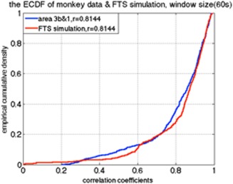
Example of the ECDF of the correlations between two sub‐regions of S1 in one monkey, along with the ECDF of the filtered stationary model simulation, KS value = 0.1280. [Color figure can be viewed at http://wileyonlinelibrary.com]

The Behavior of Connectivity in Different Monkeys

To test whether different monkeys have similar correlation trends in the same ROI pairs, VAR, filtered stationary, and underlying dynamic simulations were conducted on a single random monkey dataset. We then applied a sliding window analysis to both simulated data and the monkeys’ real fMRI data over a range of window sizes, and compared the distributions of their z‐scores using the two‐sample K‐S statistic.

RESULTS

Stationary Model Simulations

Pre‐processing of resting‐state BOLD‐fMRI time series usually includes low‐pass filtering to remove artifacts and to emphasize frequencies of interest. Such filtering, however, affects the data by introducing autocorrelations in the BOLD time series themselves [Hindriks et al., 2016]. To match the relative strength of this low‐pass filtering effect, the filtered stationary null model simulates the low‐pass filter performed on the monkey data by matching the BOLD frequency range from 0.01 to 0.1 Hz. We have found this step to be one of the most important for replicating monkey fMRI connectivity in the filtered stationary model (Supporting Information Appendix).

As expected, simulations of stationary random signals show that the variance of correlation coefficients decreases as window size increases [Hutchison et al., 2013a, 2013b]. In addition, the variance decreases for stronger correlation coefficients. The behavior of the correlation coefficients between stationary signals was similar to in vivo monkey data when using smaller window sizes, such as 60s. As shown in Figure 7, correlations between functionally related sub‐region pairs (e.g., area 3a and area 1 in the same monkey brain) of the monkey data are distributed similarly to the correlations derived from simulated stationary data for short window sizes, but depart substantially for larger window sizes such as 180s (smaller K‐S value indicates less difference).

Figure 7.

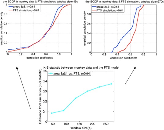
Example of the two‐sample K‐S statistic on correlations of monkey data and the filtered stationary null model simulation over a range of window sizes. [Color figure can be viewed at http://wileyonlinelibrary.com]

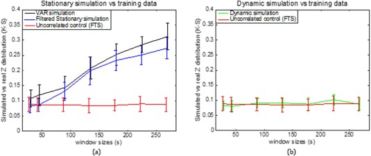
Figure 8 shows the K‐S statistic for group of cross‐correlations between two functionally related sub‐regions of S1 cortex and their corresponding models, and the K‐S statistic for cross‐correlation between functionally unrelated subregions and the filtered stationary model at the window sizes of 60s and 180s. The correlations between functionally related subregion pairs in the monkey data are distributed similarly to the correlations derived from VAR and filtered stationary models at the window size of 60s, but depart substantially at the window size of 180s. However, the correlations between functionally unrelated subregions (two sub‐regions from two different monkeys, for example, area 3a from monkey A, and area 3b from monkey B) in the monkey data are distributed similarly to the correlations derived from the filtered stationary model at both window sizes of 60s and 180s.

Figure 8.

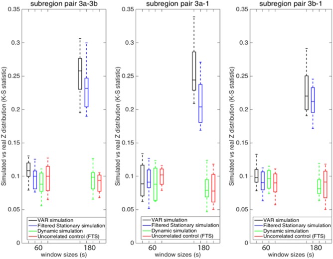
Group analysis on K‐S statistic between functionally related monkey data and the VAR, filtered stationary, underlying dynamic models, along with K‐S statistic between functionally unrelated monkey data and the filtered stationary model at window sizes 60s and 180s. Sliding window correlations in real data differed from stationary simulations only at the longer window size, as shown by the high K‐S statistic (blue, black). Introducing a dynamic component to the simulation eliminated the difference (green), meaning that correlation distributions derived from dynamic simulations matched the real data. Sliding window correlations between two different monkeys’ time series (uncorrelated by construction) were reproduced well by the stationary simulations and served as the negative control (red). Error bars indicate standard deviations. [Color figure can be viewed at http://wileyonlinelibrary.com]

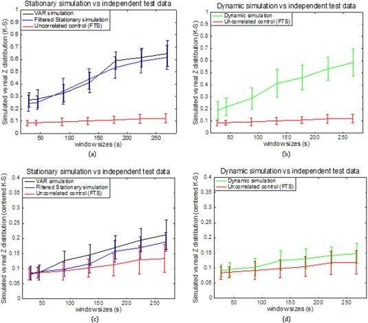
Additional window sizes can be seen in Figure 9. Figure 9a illustrates the K‐S statistic for group of cross‐correlations between two functionally related sub‐regions area 3a–3b and its corresponding stationary models. The correlations between sub‐region pair 3a–3b in the monkey data are distributed more similarly to the correlations derived from the filtered stationary null model than those derived from the VAR model. Specifically, K‐S values of correlation coefficients between area 3a–3b of the monkey data and the filtered stationary null model (blue line) are always smaller than those between the same monkey data and the VAR null model (black line). Moreover, these K‐S values increase as window sizes increase, which indicates that neither of these two stationary models matches real fMRI data very well at large window sizes. However, the correlations between functionally unrelated sub‐regions are distributed similarly to the stationary data from the filtered stationary null model simulation at all window sizes. Specifically, the red line, which represents K‐S values between unrelated sub‐regions of monkey data and the filtered stationary null model is always flat over a range of different window sizes.

Figure 9.

Group analysis on K‐S statistic between functionally related monkey sub‐region pair area 3a–3b and the stationary and dynamic models, along with K‐S statistic between functionally unrelated monkey data and the filtered stationary null model over a range of window sizes. Correlation distributions are indistinguishable from stationary simulations at the shortest window (30s) but begin to differ at longer windows (90s and up; blue and black). Dynamic simulations reproduce the correlation distributions of real data at all window sizes (green). Error bars indicate standard deviations. [Color figure can be viewed at http://wileyonlinelibrary.com]

Underlying Dynamic Model Simulation

In the dynamic correlation study, we generated an underlying dynamic null model and applied the same sliding window technique, the Fisher's z‐transform and the two‐sample K‐S statistic. Figure 9b illustrates that correlations between functionally related sub‐regions in the monkey data are distributed similarly to the correlations derived from the underlying dynamic null model at all window sizes. Specifically, the green line, which represents K‐S values between functionally related ROIs in the monkey data and the underlying dynamic null model is flat over all different window sizes.

The Behavior of Connectivity in Different Monkeys

Figure 10a,b shows a group analysis of the K‐S statistic between sub‐region pair area 3a–3b within different monkeys and the stationary and dynamic models before centering the z‐score. Figure 10c,d shows a K‐S statistic between the same subregion pair in different monkeys and three models after centering the z‐score. From Figure 10a–d, it can be seen that the K‐S values decreased dramatically after z‐score centering. This is because the average correlation coefficients of the nine datasets are different from each other, while their correlation distributions shapes are similar. From Figure 10c,d, it can be seen that the K‐S values over different window sizes are as follows: the VAR model (black line) has the largest values, followed by the filtered stationary model (blue line), followed by the dynamic model (green line), and followed by the functionally unrelated monkey data simulation (red line). The two stationary models do not capture the similar correlation features across monkeys as closely as the dynamic model. However, the underlying dynamic model is good at simulating the trend of correlation functions across all three monkeys (9 sessions).

Figure 10.

Group analysis on K‐S statistic between sub‐region pair area 3a–3b within different monkeys and the stationary and dynamic models before (a, b) and after (c, d) centering the z‐score. Error bars indicate standard deviations. [Color figure can be viewed at http://wileyonlinelibrary.com]

To verify whether dynamic correlation similarities existed within identical subregion pairs of monkey data, we plotted the four major frequency components derived from the underlying dynamic model. These components were chosen based on the underlying correlations, which were fit using a sum of four sine functions. From Figure 11, it can be seen that different monkey datasets have similar dynamic correlation frequency components within identical subregion pairs. For these three sub‐region pairs, it was observed that variation frequency components between 0 and 0.003 Hz had significant contributions to the correlation coefficients.

Figure 11.

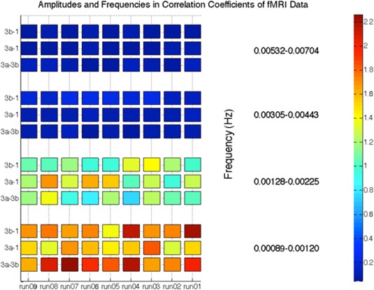
Spectral decomposition of the correlation coefficients for sub‐region pairs of area 3a–3b, 3a–1, and 3b–1. [Color figure can be viewed at http://wileyonlinelibrary.com]

DISCUSSION

The aim of this study was to investigate the existence of dynamic correlations in real fMRI data acquired from somatosensory cortex of new world monkeys. It is widely accepted that apparent variations over time may arise from stationary signals when the sample duration is finite [Kiyani and Chapman, 2009; Nason, 2006]. Considering this factor, sliding window correlation analysis should be simulated with appropriate models and statistical tests [Chang and Glover, 2010]. Based on our filtered stationary null model and the commonly used VAR model simulations for sliding window technique, we found that both stationary models reproduced the distribution of correlations of real fMRI signals well at short window sizes, but diverted at longer window sizes. This suggests that short window sizes are less reliable than long window sizes for detecting dynamic changes in functional correlations. In addition, a close representation of the behavior of resting‐state data is obtained only when a dynamic correlation is introduced, suggesting that dynamic variations in connectivity are real.

Implication for the K‐S Statistic on Correlations Between Monkey Data and the Filtered Stationary or VAR Null Model

As shown in Figures 7, 8, 9, correlations between functionally related sub‐regions in the monkey data are distributed similarly to the correlations derived from simulated stationary data at short window sizes, but depart substantially at larger window sizes. One possible explanation is that because we generated the filtered stationary null samples with only one prescribed single correlation coefficient that was calculated from the time series of the entire scan, the probability of realizing that prescribed correlation coefficient goes up as window size increases. The variance of the correlation coefficients decreases with larger window sizes, so the shape of the probability density function of correlations in the filtered stationary null model becomes narrower and taller. However, the probability density function of correlations in real fMRI data does not change as much with different window sizes, possibly because there are real dynamic changes within correlations between functionally related sub‐regions. There clearly are some characteristics of correlations between functionally related sub‐regions in the monkey data that the stationary null model cannot replicate. Given that the filtered stationary data are statistically stationary, these apparent dynamic changes at small window sizes arise from sampling variations and more rigorous analysis is required to establish the existence of dynamic changes in connectivity.

The Underlying Dynamic Null Model in Time‐Varying Correlations

As discussed above, correlations between functionally related sub‐regions in monkeys are distributed similarly to the correlations derived from both stationary null models at short window sizes, but depart substantially at larger window sizes. Simultaneously, correlations between functionally unrelated pairs in the monkey data are distributed similarly to the stationary data from the filtered stationary null model simulation at all window sizes. One explanation for this phenomenon is that correlations between functionally related sub‐regions are dynamically changing, while both stationary null models generate a static correlation through the entire series. However, for functionally unrelated sub‐region pairs, it is clear that no correlation or dynamic changes exist within the data, so our filtered stationary null model can replicate it very well over a range of window sizes. To validate this hypothesis, we generated a dynamic null model using the underlying correlation function of the monkey data, applied the same sliding window technique, z transform and the two‐sample K‐S statistic as done to other two stationary null models. Figure 9b shows that correlations between functionally related sub‐regions in the monkey data are distributed similarly to the correlations derived from the underlying dynamic null model regardless of window sizes, which indicates the underlying dynamic null model can replicate correlations between different functionally related subregions in the monkey data well. The underlying dynamic model is straightforwardly obtained by modifying the filtered stationary null model. Figure 10 indicates that the two stationary models do not simulate the trend of dynamic correlations within the monkey data. A closer representation of the behavior of monkey resting‐state data is obtained only when a dynamic correlation is introduced. Whether there are additional features within the real monkey fMRI data that are not present in the underlying dynamic model simulated data remains unclear, but exploration of additional statistical metrics is underway.

Potential Limitations concerning Sliding Window Correlation Analysis

A sliding window correlation analysis is intended to identify pairwise variations in inter‐regional time courses, but several potential limitations must be considered in applying this method and interpreting results. One limitation is that white noise can exhibit fluctuations in common functional connectivity metrics that are as large as those observed in real fMRI data. Before interpreting results about whether or not functional connectivity varies over a scan, one might need to consider whether the range of sliding window variability between ROIs is significantly different between two control populations (null model). Another limitation is the arbitrary manner in which window sizes are chosen. While many researchers tend to gravitate toward a short window size to better detect transient changes in connectivity, a large window is often necessary to allow for robust estimation of the correlation coefficient [Hutchison et al., 2013a, 2013b; Sakoglu et al., 2010]. As shown in the results of this article, a decrease in window size can lead to an overall increase in the variability of the functional connectivity since there are fewer time points available for computing correlation coefficients. Thus it will be difficult to distinguish between real phenomena related to brain signals and physiological noise. In our article, we developed a method for testing appropriate window sizes using a filtered stationary null model and K‐S statistic.

Hand–Face Region of the Primary Somatosensory Cortex (S1) of the Monkey

The S1 cortex of squirrel monkey is a unique experimental model for studies of brain activation and connectivity, with several advantages. First, the orderly topographic map of the S1 cortex serves as an anchor for our understanding of cortical organization. This orderly map is especially reflected in the hand region which is characterized by a lateral to medial representation of individual digits in three subregions of area 3a, 3b, and 1. This has been well established by studies of neuronal receptive field properties and of the effects of preferred stimuli and histological characterizations [Chen et al., 2011; Wang et al., 2013; Zhang et al., 2007]. Each area has distinct stimulus preferences, suggesting their different roles in specific somatosensory functions. In addition, stimulus evoked activations in the hand region can easily be detected and quantified in “single condition” maps. This type of quantification eliminates unnecessary ambiguities in designing orthogonal stimuli that are commonly used to reveal modular structures in the visual system. Second, Wang et al. have previously mapped the functional organization of this region at sub‐millimeter scale for touch processing, and have demonstrated that single digit fMRI activations can be reliably mapped, their responses scale with the magnitude of the vibrotactile stimuli, and confirm that digit activations are organized in a somatotopic manner. Finally, the subregions (areas 3a, 3b, and 1) of S1 cortex have been intensively mapped with electrophysiological and histological methods in this species.

Implications of Resting‐State Functional Connectivity in Primary Somatosensory Cortex

The spectral decomposition analysis for the functional connectivity of three sub‐region pairs (area 3a and 3b, area 3a and 1, area 3b and 1) has shown that the frequencies that dominated the cross‐correlation coefficients for the functionally related sub‐regions were below 0.003 Hz, which is reproducible across sub‐region pairs and subjects. This may indicate that fluctuations in resting‐state functional connectivity in primary somatosensory cortex are very slow.

CONCLUSION

The filtered stationary null model that we developed is not derived from any specific fMRI data but requires knowledge only of a correlation coefficient that is calculated from the time series of the entire scan. From our results, the dynamic model matches the real monkey fMRI data well and significantly supports the exploration of underlying correlations. Moreover, analysis of dynamic components shows that variation frequency components between 0 and 0.003 Hz contribute significantly to the correlation coefficients, which indicates that variations in resting‐state primary somatosensory cortex functional connectivity are very slow. In addition, time series generated by the filtered stationary null model appear to behave very similar to real fMRI data from S1 of monkey cortex, and exhibit dynamic changes when analyzed using the sliding window technique. Sliding window estimates of variations in correlation between non‐stationary signals may reveal dynamic changes but also may be confounded by statistical variations. While stationary models replicate several features of real data, a closer representation of the behavior of resting‐state data acquired from S1 in new world monkeys is obtained only when an underlying dynamic or non‐stationary correlation is introduced. This suggests that dynamic changes in resting‐state connectivity within the primary somatosensory cortex of non‐human primates are not artifacts of limited sampling duration.

Supporting information

Supporting Information Appendix.

REFERENCES

- Achard S, Salvador R, Whitcher B, Suckling J, Bullmore E (2006): A resilient, low‐frequency, small‐world human brain functional network with highly connected association cortical hubs. J Neurosci 26:63–72. [DOI] [PMC free article] [PubMed] [Google Scholar]
- Allen EA, Damaraju E, Plis SM, Erhardt EB, Eichele T, Calhoun VD (2014): Tracking whole‐brain connectivity dynamics in the resting state. Cereb Cortex 24:663–676. [DOI] [PMC free article] [PubMed] [Google Scholar]
- Beckmann CF, DeLuca M, Devlin JT, Smith SM (2005): Investigations into resting‐state connectivity using independent component analysis. Philos Trans R Soc Lond B Biol Sci 360:1001–1013. [DOI] [PMC free article] [PubMed] [Google Scholar]
- Biswal B, Yetkin FZ, Haughton VM, Hyde JS (1995): Functional connectivity in the motor cortex of resting human brain using echo‐planar MRI. Magn Reson Med 34:537–541. [DOI] [PubMed] [Google Scholar]
- Chakravarti, Laha, Roy (1967): Handbook of Methods of Applied Statistics, Volume I. John Wiley and Sons, pp. 392–394. [Google Scholar]
- Chang C, Glover GH (2010): Time‐frequency dynamics of resting‐state brain connectivity measured with fMRI. Neuroimage 50:81–98. [DOI] [PMC free article] [PubMed] [Google Scholar]
- Chen LM, Turner GH, Friedman RM, Zhang N, Gore JC, Roe AW, Avison MJ (2007): High‐resolution maps of real and illusory tactile activation in primary somatosensory cortex in individual monkeys with functional Magn Reson Imaging and optical imaging. J Neurosci 27:9181–9191. [DOI] [PMC free article] [PubMed] [Google Scholar]
- Chen L, Mishra A, Newton AT, Morgan VL, Stringer EA, Rogers BP, Gore JC (2011): Fine‐scale functional connectivity in somatosensory cortex revealed by high‐resolution fMRI. Magn Reson Imaging 29:1330–1337. [DOI] [PMC free article] [PubMed] [Google Scholar]
- Cordes D, Haughton VM, Arfanakis K, Wendt GJ, Turski PA, Moritz CH, Quigley MA, Meyerand ME (2000): Mapping functionally related regions of brain with functional connectivity MR imaging. AJNR Am J Neuroradiol 21:1636–1644. [PMC free article] [PubMed] [Google Scholar]
- Cribben I, Wager TD, Lindquist MA (2013): Detecting functional connectivity change points for single‐subject fMRI data. Front Comput Neurosci 7:143. [DOI] [PMC free article] [PubMed] [Google Scholar]
- Damoiseaux JS, Rombouts SA, Barkhof F, Scheltens P, Stam CJ, Smith SM, Beckmann CF (2006): Consistent resting‐state networks across healthy subjects. Proc Natl Acad Sci USA 103:13848–13853. [DOI] [PMC free article] [PubMed] [Google Scholar]
- Dosenbach NU, Fair DA, Miezin FM, Cohen AL, Wenger KK, Dosenbach RA, Fox MD, Snyder AZ, Vincent JL, Raichle ME, Schlaggar BL, Petersen SE (2007): Distinct brain networks for adaptive and stable task control in humans. Proc Natl Acad Sci U S A 104:11073–11078. [DOI] [PMC free article] [PubMed] [Google Scholar]
- Fox MD, Snyder AZ, Vincent JL, Corbetta M, Van Essen DC, Raichle ME (2005): The human brain is intrinsically organized into dynamic, anticorrelated functional networks. Proc Natl Acad Sci USA 102:9673–9678. [DOI] [PMC free article] [PubMed] [Google Scholar]
- Fransson P (2005): Spontaneous low‐frequency BOLD signal fluctuations: An fMRI investigation of the resting‐state default mode of brain function hypothesis. Hum Brain Mapp 26:15–29. [DOI] [PMC free article] [PubMed] [Google Scholar]
- Friedman RM, Dillenburger BC, Wang F, Avison MJ, Gore JC, Roe AW, Chen LM (2011): Methods for fine scale functional imaging of tactile motion in human and nonhuman primates. Open Neuroimag J 5:160–171. [DOI] [PMC free article] [PubMed] [Google Scholar]
- Friston KJ, Buechel C, Fink GR, Morris J, Rolls E, Dolan RJ (1997): Psychophysiological and modulatory interactions in neuroimaging. NeuroImage 6:218–229. [DOI] [PubMed] [Google Scholar]
- Greicius MD, Krasnow B, Reiss AL, Menon V (2003): Functional connectivity in the resting brain: A network analysis of the default mode hypothesis. Proc Natl Acad Sci USA 100:253–258. [DOI] [PMC free article] [PubMed] [Google Scholar]
- Hacker RS, Hatemi‐J A (2005): A test for multivariate ARCH effects. Appl Econ Lett 12:411–417. [Google Scholar]
- Handwerker DA, Roopchansingh V, Gonzalez‐Castillo J, Bandettini PA (2012): Periodic changes in fMRI connectivity. Neuroimage 63:1712–1719. [DOI] [PMC free article] [PubMed] [Google Scholar]
- Hindriks R, Adhikari MH, Murayama Y, Ganzetti M, Mantini D, Logothetis NK, Deco G (2016): Can sliding‐window correlations reveal dynamic functional connectivity in resting‐state fMRI? Neuroimage 127:242–256. [DOI] [PMC free article] [PubMed] [Google Scholar]
- Hutchison RM, Womelsdorf T, Allen EA, Bandettini PA, Calhoun VD, Corbetta M, Della Penna S, Duyn JH, Glover GH, Gonzalez‐Castillo J, Handwerker DA, Keilholz S, Kiviniemi V, Leopold DA, de Pasquale F, Sporns O, Walter M, Chang C (2013a): Dynamic functional connectivity: Promise, issues, and interpretations. Neuroimage 80:360–378. [DOI] [PMC free article] [PubMed] [Google Scholar]
- Hutchison RM, Womelsdorf T, Gati JS, Everling S, Menon RS (2013b): Resting‐state networks show dynamic functional connectivity in awake humans and anesthetized macaques. Hum Brain Mapp 34:2154–2177. [DOI] [PMC free article] [PubMed] [Google Scholar]
- Jones DT, Vemuri P, Murphy MC, Gunter JL, Senjem ML, Machulda MM, Przybelski SA, Gregg BE, Kantarci K, Knopman DS, Boeve BF, Petersen RC, Jack CR Jr. (2012): Non‐stationarity in the “resting brain's” modular architecture. PLoS One 7:e39731. [DOI] [PMC free article] [PubMed] [Google Scholar]
- Kiyani KH, Chapman SC (2009): Pseudononstationarity in the scaling exponents of finite‐interval time series. Phys Rev E 79:036109. [DOI] [PubMed] [Google Scholar]
- Lowe MJ, Mock BJ, Sorenson JA (1998). Functional connectivity in single and multislice echoplanar imaging using resting‐state fluctuations. Neuroimage 7:119–132. [DOI] [PubMed] [Google Scholar]
- Marsaglia G, Tsang WW, Wang J (2003): Evaluating Kolmogorov's Distribution. J Stat Softw 8:1–4. [Google Scholar]
- McKeown MJ, Makeig S, Brown GG, Jung TP, Kindermann SS, Bell AJ, Sejnowski TJ (1998): Analysis of fMRI data by blind separation into independent spatial components. Hum Brain Mapp 6:160–188. [DOI] [PMC free article] [PubMed] [Google Scholar]
- Mezer A, Yovel Y, Pasternak O, Gorfine T, Assaf Y (2009): Cluster analysis of resting‐state fMRI time series. Neuroimage 45:1117–1125. [DOI] [PubMed] [Google Scholar]
- Nason GP (2006): Stationary and non‐stationary time series In: Mader H, Coles SC, editors. Statistics in Volcanology. The Geological Society, p. 129–142. Chapter 11. [Google Scholar]
- Power JD, Cohen AL, Nelson SM, Wig GS, Barnes KA, Church JA, Vogel AC, Laumann TO, Miezin FM, Schlaggar BL, Petersen SE (2011): Functional network organization of the human brain. Neuron 72:665–678. [DOI] [PMC free article] [PubMed] [Google Scholar]
- Sakoglu U, Pearlson GD, Kiehl KA, Wang YM, Michael AM, Calhoun VD (2010): A method for evaluating dynamic functional network connectivity and task‐modulation: Application to schizophrenia. Magma 23:351–366. [DOI] [PMC free article] [PubMed] [Google Scholar]
- Shah A, Khalid MU, Seghouane AK (2012): Comparing causality measures of fMRI data using PCA, CCA and vector autoregressive modelling. Conf Proc IEEE Eng Med Biol Soc 2012:6184–6187. [DOI] [PubMed] [Google Scholar]
- Stephens MA (1974): Edf statistics for goodness of fit and some comparisons. J Am Stat Assoc 69:730–737. [Google Scholar]
- Sun FT, Miller LM, D'Esposito M (2005): Measuring temporal dynamics of functional networks using phase spectrum of fMRI data. Neuroimage 28:227–237. [DOI] [PubMed] [Google Scholar]
- Wang Z, Chen LM, Negyessy L, Friedman RM, Mishra A, Gore JC, Roe AW (2013): The relationship of anatomical and functional connectivity to resting‐state connectivity in primate somatosensory cortex. Neuron 78:1116–1126. [DOI] [PMC free article] [PubMed] [Google Scholar]
- Yeo BT, Krienen FM, Sepulcre J, Sabuncu MR, Lashkari D, Hollinshead M, Roffman JL, Smoller JW, Zollei L, Polimeni JR, Fischl B, Liu H, Buckner RL. (2011): The organization of the human cerebral cortex estimated by intrinsic functional connectivity. J Neurophysiol 106:1125–1165. [DOI] [PMC free article] [PubMed] [Google Scholar]
- Zalesky A, Fornito A, Cocchi L, Gollo LL, Breakspear M (2014): Time‐resolved resting‐state brain networks. Proc Natl Acad Sci USA 111:10341–10346. [DOI] [PMC free article] [PubMed] [Google Scholar]
- Zhang N, Gore JC, Chen LM, Avison MJ (2007): Dependence of BOLD signal change on tactile stimulus intensity in SI of primates. Magn Reson Imaging 25:784–794. [DOI] [PubMed] [Google Scholar]
Associated Data
This section collects any data citations, data availability statements, or supplementary materials included in this article.
Supplementary Materials