Review of General Algorithmic Features for Genome Assemblers for Next Generation Sequencers

Abstract

In the realm of bioinformatics and computational biology, the most rudimentary data upon which all the analysis is built is the sequence data of genes, proteins and RNA. The sequence data of the entire genome is the solution to the genome assembly problem. The scope of this contribution is to provide an overview on the art of problem-solving applied within the domain of genome assembly in the next-generation sequencing (NGS) platforms. This article discusses the major genome assemblers that were proposed in the literature during the past decade by outlining their basic working principles. It is intended to act as a qualitative, not a quantitative, tutorial to all working on genome assemblers pertaining to the next generation of sequencers. We discuss the theoretical aspects of various genome assemblers, identifying their working schemes. We also discuss briefly the direction in which the area is headed towards along with discussing core issues on software simplicity.

Introduction

Genome assembly is very similar to solving a jigsaw puzzle. In a jigsaw puzzle, one has a large number of pieces and access to the final picture that essentially tells where each piece must be placed. In spite of having the complete picture, which is the prior knowledge that tells us how each and every individual piece connects to one another, we all know how difficult and time-consuming it is to solve this very jigsaw puzzle. Imagine now that we do not know the final product, the complete picture. Rather all we have are the individual pieces. Imagine how difficult would it be now to solve this problem. Genome assembly is the exact same problem. Here we have a vast number of individual pieces, called reads, and we do not know how to connect them all together since we do not know the final product, the sequence.

The data associated with genome assembly comes from a variety of platforms. Development of the next-generation sequencing (NGS) platforms sparked the need for algorithms that could cater for the immense amount of data produced by these platforms. Figure 1 sketches chronologically the major developments in the last decade. As suggested by Figure 1, the scope and aim of this paper is to qualitatively communicate all the problem-solving strategies and algorithms that are employed by NGS platforms. Earlier assembly algorithms, not related to NGS, like AssemblyLIGN [1], CCG (http://www.health.usf.edu/library/gcg.html), GeneWorks [2], AutoAssembler [3], Seqman [4], Sequencher [5], GENeration (Intelligenetics), PC/Gene (Intelligenetics) (ftp://193.62.192.4/pub/databases/info/ig_prod.txt), FAB [6] and XBAP [7] are surveyed in [8], while algorithms developed for Sanger technology [9] like Phrap [10], TIGR [11], Celera [12], Arachne [13] and CAP3 [14] are surveyed in [15]. It is also intended that the readers of this paper could tap from the gold mine of algorithms that can solve jigsaw problems, fine tune them and solve the task of genome assembly in a much better fashion.

Figure 1.

Leading advancements in sequencing schemes during 2000–2010 Please note that this figure is not an exhaustive list, but it lists the major developments.

The rest of this paper is organized as follows. The types of genome assembly and the problems it faces are described under Genome assembly paradigms. Fundamental schemes section discusses the various schemes used by different algorithms to solve the genome assembly problem and provides an insight into the working schemes of the algorithms shown in Figure 1. The direction in which this area is moving and core issues in software simplicity will be briefly discussed at the end of this review.

Genome assembly paradigms

The strategy adopted by genome assemblers can be widely divided into two categories: comparative assembly and de novo assembly. Looking back at the analogy with the jigsaw puzzle, if no knowledge is available about the end product, i.e., the complete final picture which is made by putting all the pieces together in the right order, then that is de novo assembly. However, if one has access to the complete or partial picture of the final product, e.g., only this time a toddler has colored over, distorted or torn apart the puzzle’s pieces from some edges, then that is comparative assembly. Even though the toddler distorted the image, in the case of genome assembly, the specimen happens to be the reference sequence, may be distorted, yet it provides a great help to the scientists because it eases the task of putting the pieces together in the right place given the fact that there are a massive number of reads that need to be ordered properly. In other words, comparative assembly uses a reference sequence for genome assembly whereas de novo assembly does not. Thus de novo assembly is more complicated than comparative assembly.

The question that remains is how to choose a reference sequence? If the DNA to be sequenced is a unique genome unlike others that have been referenced or the only one in its class, then it is best to adopt a de novo assembly scheme. However, if the DNA to be sequenced has closely related strains whose sequences are already known, then it is best to use the known sequences as its reference template. What defines a closely related strain can be explained from where the DNA in question comes from. If the DNA comes from a laboratory strain then sequencing is generally done on mutant strains which are derived from some parental strain. All these strains, parental and mutant, are isogenic in nature, meaning they present the same genes. If the DNA is a clinical isolate, wild type DNA, isolated directly from nature and not modified in any manner, then the reference can come from other DNA sequences belonging to the same species or closer DNA having the same spoligotype information. Spoligotype is the equivalent of a fingerprint of the family of strains that share the same repeat units of a DNA. The reference sequence, if possible, should belong to the same family of strains. However, spoligotyping is only applicable for tuberculosis [16], [17], [18], [19], [20].

Genome assembly could also be categorized in accordance to the sequencing platform it uses to generate the data. Some platforms are Sanger, Illumina, Roche 454 and Applied Bio-systems [21], [22], [23], [24]. The Sanger method was the de facto standard for DNA sequencing. It was also used in the Human Genome Project. NGS has five platforms that are available. Still newer platforms are underway since the US National Human Genome Research Institute (NHGRI) announced funding for a series of projects to achieve sequencing of a human genome for under $1000. The input to these platforms is the DNA whose sequence is unknown. The output, amongst other things, is a massive set of reads that need to be ordered and combined in order to identify the unknown sequence. The read itself is a sequence of letters: A, T, G, C or N, whose length is fixed and is determined by the platform used for sequencing.

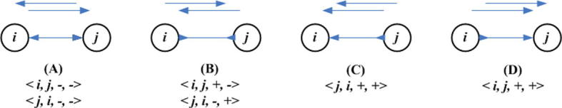
Not only is the jigsaw puzzle difficult to resolve, but also, there are other problems that genome assembly faces. Genome assembly is plagued with low coverage areas, avoiding false positive read-read alignments (caused by chimeric reads), avoiding false negative alignments (missing read–read alignments), poor sequence quality, polymorphism (having multiple alleles, or slightly modified versions of the same gene) and repeated regions in genome. These problems can be reduced by using similar genomes. Another issue that all assemblers have to face is that a read consists of two strands that are reverse complements of each other. Whenever DNA is sequenced, the molecule is always read in the same direction, from 5′ to 3′, but it is impossible to know from which of the two strands the sequence is read. In this regard, two popular paradigms known amongst the designers of these assemblers are ‘overlap-layout-consensus’ and ‘alignment-layout-consensus’.

Fundamental schemes

The most fundamental schemes used in genome assemblers are the overlap-layout-consensus, alignment-layout-consensus, the greedy approach, graph-based schemes and the Eulerian path. Figure 2 lists the respective algorithms and their associated schemes. However, it should be noted that these schemes are not exclusive and one algorithm can be categorized in more than one scheme. An example of different yet not exclusive schemes is the comparative and the de novo assembly mechanism. Although comparative assembly uses the reference sequence for alignment of reads, yet reads corresponding to the areas of the novel genome that differ significantly with respect to the reference genome need to be connected via de novo assembly [25]. The remainder of this section explains these basic schemes one by one.

Figure 2.

Schemes and their associated algorithms The figure depicts the most fundamental schemes adopted by assembly algorithms. The algorithms have been listed in order to clarify fundamental concepts; however, the same algorithm can be categorized into more than one approach. For instance, all Eulerian path approach algorithms could be categorized under graph-based schemes. However, assisted assembly can be categorized under both comparative assembly and the overlap-layout-consensus approach since it uses concepts from both.

The greedy approach works by making the locally optimal choice at each stage with the hope of finding the global optimum [26]. It starts with a contiguous sequence, a contig, by taking an unassembled read, and extends it by using the current read’s best overlapping read on its 3′ end. If the contig cannot be extended further, the process is repeated at the 5′ end of the reverse complement of the contig.

The overlap-layout-consensus, as the name suggests, consists of three steps (see Supplementary section, [27]). In the first step an overlap graph is created by joining all the reads by their respective best overlapping reads. This step is similar to the greedy approach. The layout stage, ideally, is responsible for finding one single path from the start of the genome traversing through all the reads exactly once and reaching the end of the sequenced genome. This ideal scenario is not always achievable and is the reason why we have so many algorithms trying to find the solution using the same scheme. The layout stage is carried out in a hierarchical fashion. Celera Assembler [12], for instance, starts by identifying all unique contigs called ‘unitigs’. These unitigs are regions of the genome that are generated perfectly via the assembly process. Unitigs connect equally well with more than one contigs. There are various ways to settle potential disputes as to which contig the unitig would connect to in order to elongate the size of the contig. For example, Celera and Arachne [13] use mate-pair information to merge sets of unitigs to form larger contigs. In the consensus stage, groups of reads that overlapped now cast their votes in order to identify which base should be present at a particular location of the novel genome. A major part of the literature is dedicated to using the overlap-layout-consensus paradigm via the concepts of graph theory. Therefore, the graph theory approach is not an independent approach as it shares common grounds with other schemes to solve the genome assembly problem.

Concepts like string graphs, bidirected graphs and de Bruijn graphs have had a deep impact on assembly algorithms [28], [29], [30], [31], [32], [33], [34], [35]. The aim of all assemblers based on graph theory is to represent reads as a set of nodes, and overlaps between these reads as directed edges which connect these nodes to form a complete graph via a Hamiltonian path or an Eulerian path [36], [37]. For a Hamiltonian path, each node in the graph is traversed only once, while for an Eulerian path, all edges but not nodes are traversed exactly once. So an Eulerian path may traverse a given node more than once.

However, whenever graph theory is employed to resolve genome assembly, it faces certain dilemmas. It is one thing to make a graph, and it is another thing to simplify it. Ideally speaking, one should obtain one graph where there is only one path from root to child node and that path should signify the genome sequence itself. However, it is never the case. The initial phase of the assembly provides, not one, but several smaller disjoint graphs. These smaller disjoint graphs need to be connected to one another to form one large graph. A path from a root node to a child node in each one of these disjointed graphs corresponds to a contig. Each disjointed graph is composed of many branches. Every branch or loop in the graph is a potential hazard for the program as it could signify repeat regions in the genome. If these loops do signify repeat regions then one has to decide where to place them along the genome. Some branches are short and can be discarded while others are responsible for longer paths which end up competing with one another in defining the contig. The branches are usually caused by read data which present errors, as the NGS platforms do not provide perfect read data from the genome sequences. Furthermore, these disjointed graphs, or contigs, need to be connected in some manner, an operation called scaffolding, in order to converge to the final assembly of the genome sequence (see Supplementary section) [27]. Therefore, all assemblers that exploit graph theory inherently employ an extensive graph simplification process in order to simplify identifying the contigs and subsequently implementing scaffolding [38], [39], [40]. Figure 3 discusses various ways via which graph simplification is carried out.

Figure 3.

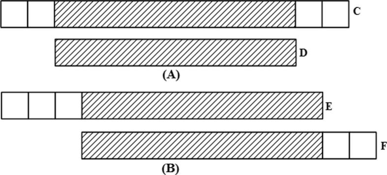
Graph correction techniques (A) Disambiguation: the loop edge is unrolled and integrated in the continuous edge from left to right. (B) Pulling apart operation: the case shown could have four possible options as shown in panel (C–F). However, it is assumed here that there are only two possible paths as shown in (C) and (F), black going to black, and shaded region going to shaded region respectively, in which case the middle sequence (black) is duplicated and the two disconnected paths are made. (C–F) Eulerian super-path to eulerian path transformation: solving repeats. Repeats create difficulties since the algorithm cannot identify the correct path whether the path is shown is (C, D, E or F), respectively. Two paths are consistent if their union is a path again. For multiple edges there are 3 possibilities: (i) Path X, shown above, is consistent with exactly one of the sets in (C or D), as there is only one solution; (ii) X is consistent with neither of paths shown in (C or D); (iii) X is consistent with both (C and D). (ii) and (iii) are resolved after determining (i) for the entire graph and removing all poor quality reads. (G) Removing nodes: nodes that have an indegree = outdegree = 1 are collapsed to form one giant node called unitig. (H) Removing edges: an edge between (A and C) is removed if edges between (A and C), or (C and C), exist. (I) Velvet – removing tips: a tip is defined as a chain of nodes that is disconnected at one end. Tips are removed based upon length and minority count. If a tip is smaller than 2 k, then it is removed. Minority count property suggests the point at which the tip connects to the graph (the parent from which initial branching took place); if there is a longer path, or a more common path, then the tip is removed. In this case c is removed. Edena-dead-end path removal: similar to removing tips, here each path starting from a branching node is checked to see whether its depth is greater than $\Upsilon$ or not. Heuristically, $\Upsilon$ = 10. If not, then all the nodes in the path, excluding the branching node, are removed. These short paths are normally caused by base calling errors. (J) E₁ − E₂ – detachment: edges E₁ and E₂ are replaced by a new edge E₃ that directs all paths from V_in to V_out. (K) Removal of transitive edges: if E₁ < E₂ such that edge E₁ is overlapped by E₂, then E₁ is a transitive edge and is removed.

The last scheme that needs to be discussed is the comparative assembly, which uses the alignment-layout-consensus paradigm. The use of reference sequence, if available, allows relatively easy construction of the novel genome. Scaffolding is inherent in the procedure. Location along the reference genome where the contigs align defines the relative placement of the contigs [25], [27].

Celera

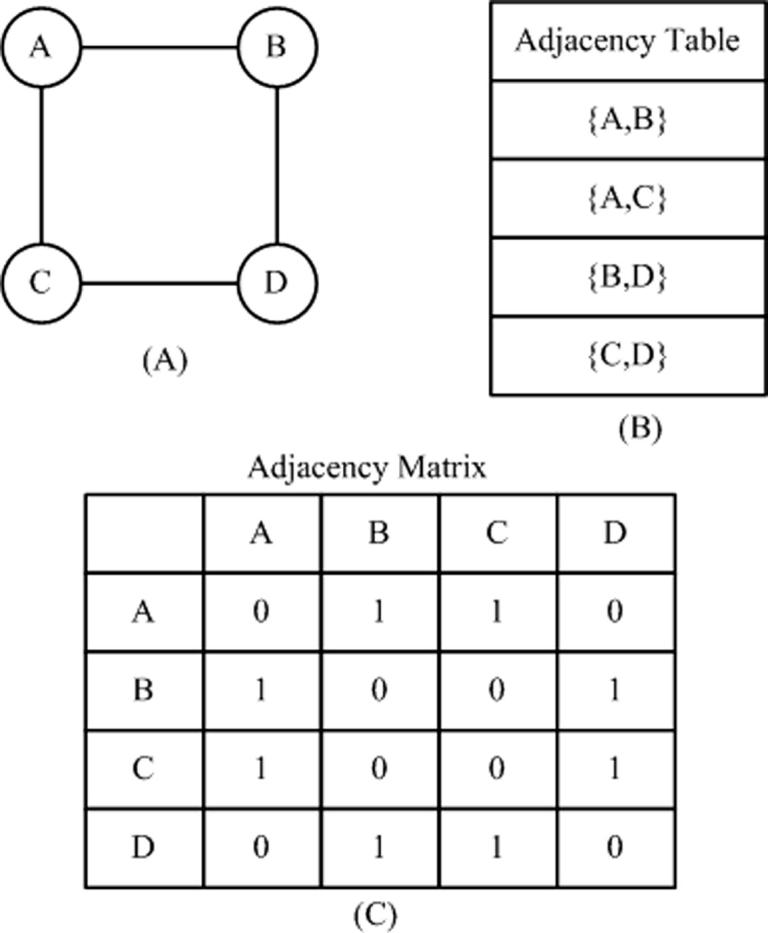
Graph theory has been extensively used for genome assembly. A graph is a data structure $\mathcal{G}$ consisting of a set of nodes $\mathcal{N}=\{N_1\text{,}\dots \text{,}{N}_n\}$ and a set of edges ε. A graph may be directed, if all the edges are oriented N_i → N_j. It is undirected if all edges do not assume any orientation $N_i\leftrightharpoons \mathit{Nj}$ or $N_i-N_j$. Genome assembly is looked upon as a graph structure with known nodes and unknown edges. The nodes are the reads and how they are connected is denoted in terms of the graph edges [41].

Celera Assembler [12] is a de facto standard in promoting large-scale genome assembly of reads. Each assembly process starts with a filtering process where low quality reads are removed. This is necessary in order to keep the rate of false overlap low [12]. The screening process by Celera involved matching reads with known ribosomal and heterochromatin DNA. Reads that matched were removed whereby these regions of DNA were not assembled.

Reads were then compared with one another to find overlapping reads that matched more than τ number of bases. For a high τ, such as τ = 94%, it meant that such overlap is either true or is caused by a repeat. Unique overlapping reads were combined together to form contiguous sequence called U-unitigs if the overlap was a true-overlap and just unitig if they may belong to repeat regions, where a unitig is a maximal interval subgraph [42], [43], [44], [45].

Repeats resolution is done at this stage by dynamic programming [46], [47], [48], [49]. Repeats are detected by finding if unitig X happens to overlap both Y and Z [27]. Thereafter, scaffolding is done which identifies the relative placement and ordering of the unitigs with respect to one another. Scaffolding is done by mate-pair information when left and right reads happen to be present in different unitigs followed by aggressive repeat resolution measures.

The consensus sequence is generated by looking at the base calls in each column and the confidence of each base-call is identified using the quality values (Q values) provided by each base (see Supplementary section, [27]).

Eulerian path approach

An Eulerian approach uses the reads to form a de Bruijn graph (see Supplementary section, [27]). Since each read has a fixed number of bases or nucleotides l, they are interchangeably referred to as a l-tuple or a l-mer. If two l-tuples N₁ and N₂ overlap such that the last l − 1 bases of N₁ overlap with the first l − 1 bases of N₂, then a directed edge is formed N₁ → N₂. Repeating the same process over the collection of reads S₁, … , S_n and its reverse complement $S_1^c\text{,}\dots \text{,}{S}_n^c$, called the spectrum $\mathcal{S}$, generates a graph, a process referred to as the spectral alignment problem. As $\mathcal{S}$ contains a complement of every read, the graph can be partitioned into two subgraphs: one corresponding to the set of reads S₁, … , S_n and the other one pertaining to the complement set $S_1^c\text{,}\dots \text{,}{S}_n^c$. This helps in eliminating the false edges in the graph greatly. Furthermore, employing multiple alignments of l-tuples as opposed to pairwise alignments helps also to reduce the number of errors.

In graph theory language, the set of nodes N₁, … , N_k forms a path if for every i ∈ {1, … , k − 1} we have either N_i → N_i+1 or N_i ← N_i+1, i.e., an edge exists between any two consecutive nodes in the path. The path is directed if there exists at least one directed edge between any two consecutive nodes N_j → N_j+1. Genome assembly via EULER [50] presumes to identify an Eulerian path, which traverses all the edges of $\mathcal{G}$ exactly once as described previously. In the attempt to resolve the genome assembly problem via the Eulerian path one does not end up with a single path but with multiple paths. Therefore, the solution to the problem lies in finding an Eulerian super-path that contains all these Eulerian paths as sub-paths (see Supplementary section) [27].

De novo assembly with A-Bruijn graphs

A follow up to the Eulerian path approach which uses de Bruijn graphs is the usage of A-Bruijn graphs, which are a generalized version of de Bruijin graphs for genome assembly [51]. An A-Bruijn graph is formed using a similarity matrix (see Supplementary section, [27]).

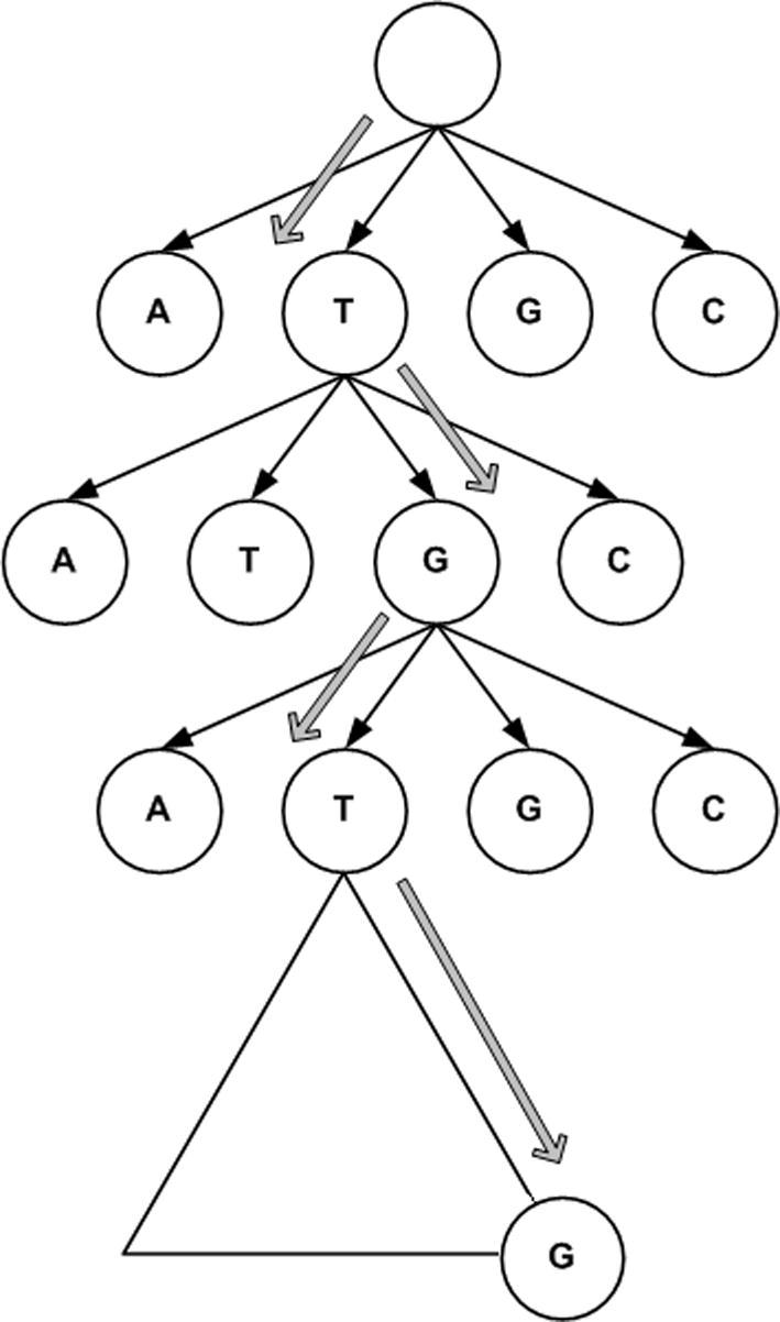
In genome assembly, the l-tuple or l-mer is basically the read or its reverse complement. After removing low quality reads, the similarity matrix is then employed to define the adjacencies to all perfect l-mers. If the genomic sequence of length n is unknown, yet a set of sub-strings ${\mathcal{S}}_1\text{,}{\mathcal{S}}_2\text{,}\dots \text{,}{\mathcal{S}}_k$ that span the entire length n is known, an n × n similarity matrix $\mathcal{A}$ can be made from the $\frac{k(k-1)}{2}$ pair-wise alignments [51], [52], [53], [54], [55], [56]. Using this similarity matrix $\mathcal{A}$, an A-Bruijn graph $\mathcal{G}$($\mathcal{V}$,ε) is constructed. Herein $\mathcal{V}$ denotes the set of connected vertices or nodes. All vertices that are similar to one another are collapsed into one vertex, as illustrated by Figure 4. An Eulerian path traversing from vertex₁ to vertex_n represents the edges, and it is indicated in the form of the set ε in the graph $\mathcal{G}$. All these operations are graphically depicted in Figure 4.

Figure 4.

Making the A-Bruijn graphs (A) Using pair-wise alignments an A-Bruijn graph $\mathcal{G}$ is built from the sequence. (B) Pair-wise alignments are calculated: ATG versus AT, while in (C), it is AT versus AAG and ATG versus AAG. (D) Final assembly of the A-Bruijn graph $\mathcal{G}$ after collapsing all similar nodes. Resultant graph may contain whirls and bulges which need to be rectified. Herein, A → T ← A is a whirl. (E) In the event of a mismatch, two nodes are collapsed and both instances are kept. Figure was adapted from [51].

Graph simplification and genome assembly

The pair-wise alignments $\mathcal{A}$ and the graph $\mathcal{G}$ present mismatches as illustrated in Figure 4 in terms of whirls and bulges. A whirl is a small cycle that has edges in the same direction, whereas bulges are small cycles that contain edges in either direction. Graph simplification helps in removing these ailments.

Whirls are caused by ambiguities in pair-wise alignments. Whirls can be removed by putting gaps or removing some matches in the alignment [27]. Bulges are more difficult to remove. They can be resolved by adopting the maximum weighted spanning tree strategy [27], [57], [58], [59], [60].

Thereafter, tips and branches that are shorter in length are removed (Figure 3I). This process is also called erosion in EULER, EULER-SR and A-Bruijn graph assembly terminology [38], [51], [52], [53], [61]. The graph obtained after all these simplification techniques presents some long simple paths yet an important question remains unresolved. What is the consensus sequence of these individual paths? Basically the most frequently occurring base happens to be the consensus base which helps to define the consensus sequence of these long simple paths. To identify that, the coverage of each path or the average coverage of each vertex is evaluated, which helps in identifying the consensus sequence for each path. The coverage of the vertex is the number of reads that traverse through that vertex. Note that there may be different bases that occur at any one given position due to mismatches within different copies of repeats and so a consensus for every position is required to determine the right nucleotide at that position. These simple paths are then collapsed to form a repeat graph whose edges are the consensus sequences of the corresponding simple paths. These edges are basically the contigs. Scaffolding of these contigs is done in the same manner as in EULER [50].

EULER-SR

EULER-SR [52] fine tunes EULER to assemble short reads more efficiently. Its extensive pre-processing stage and more thorough graph correction schemes make EULER-SR more efficient to handle short read assemblies than EULER. In the pre-processing stage, reads that are not valid are removed. In EULER-SR, the pre-processing stage is called the “error correction stage” because it focuses not only on removing reads that are not valid but also, if possible, removing errors from the reads and making them useful in the genome assembly process. Q values are used to discard low-quality reads. In the absence of Q values, the spectrum S [27] is employed for error correction. All reads (k-mers) in S are divided into l-tuples, a sub-string of size l. All l-tuples whose frequency in S is above a certain threshold are kept and the rest are discarded. The reads which these tuples belong to are modified to account for the remaining tuples. If the number of changes required for any read is greater than a certain threshold, it is discarded.

After error correction, the remaining reads are used for the formation of the de Bruijn graph. In EULER-SR, the de Bruijn graph obtained at the end of the entire assembly process contains O(L) nodes and O(L) edges for a target genome of length L, regardless of the number of reads in the data set. Graph construction is similar to EULER. Edges between two nodes, adjacencies, are found by doing a binary search for every adjacent pair of nodes in spectrum S [62], [63], [64], [65], [66]. Since reads are used in the formation of the de Bruijin graph, a weight equal to the number of reads mapped to the edge is assigned to each edge. This weight helps in eliminating chimeric reads (see Supplementary section, [27]). After simplification, every l + 1 tuple in the read maps to a unique position and edge in the graph.

The graph needs to be corrected after being made. Graph correction can be defined as the process where a graph $\mathcal{G}$ is transformed into a graph $\widehat{\mathcal{G}}$ which contains a subset of the vertices and edges of the graph $\mathcal{G}$. Individual reads were divided into l-tuples, therefore, a single mutation in a read causes l extra edge in the de Bruijn graph. The scope of graph correction is to eliminate extra edges and nodes, and to obtain a graph containing O(L) nodes and O(L) edges for a target genome of length L.

Graph simplification also, involves repeat resolution (Figure 3C–F, J, K)), which is similar to EULER. Repeats that are very similar are merged into a single edge corresponding to the repeat consensus sequence. Graph correction contains a separate path for each distinct repeat sequence, so in terms of graph theory it removes all erroneous edges.

Tandem repeats are identified by areas of the genome where a particular sequence repeats itself over and over again in tandem. Identifying the number of copies (multiplicity) in a tandem repeat is a difficult problem for any assembler. For de Bruijn graphs, the multiplicity of perfect tandem repeats of length longer than half of the read length cannot be inferred. Therefore, only two copies of the perfect tandem repeat are allowed and a path is constructed that traverses the repeat twice [52].

In addition, reads that were mapped to edges deleted during the graph correction stage are threaded through the nearby remaining edges by finding a path P that is sufficiently similar to the deleted edge and then putting P in place of the deleted edge. Chimeric reads are eliminated via erosion [51]. Erosion involves removing short branches that terminate quickly (Figure 3I), and removing low-weight edges. The resultant paths in the graph after graph correction are the contigs.

ALLPATHS

ALLPATHS [67], [68] assembler is amongst the list of assemblers that rely on graph theory for de novo genome assembly. It uses the spectrum to generate the graph, also called the ‘sequence graph’. The sequence graph follows a thorough and extensive simplification mechanism to reduce the graph so that there are only a few or no branches. Lastly, scaffolding is done to connect all sub-graphs or contigs to achieve global assembly.

Error correction

Error correction schemes aim to use only a subset of all the reads for assembling the genome. It first identifies low quality reads and then improves them using some heuristics. If the quality of these reads improves, they are retained for assembly. Otherwise, they are discarded. ALLPATHS has a unique method for keeping, modifying or discarding reads. It creates a list of all k-mers from the reads. It then calculates the following function $f(m)={\sum }_{i=1}^{n}l[\text{Number of times}k\text{-}{\text{mer}}_i\text{occurs}]=m$. It means that for any given k-mer if it occurs m times then it is counted in the sum f(m). f(m) = n means that there are n distinct k-mers which occur ‘m’ times. The essence behind using such a function, f(m), is to identify k-mers that occur more frequently. For f(m) = n, the aim is to use all n distinct k-mers that occur m times. A simple graph is made with x = m and y = f(m) to identify the confident k-mers from the weak k-mers, where confident k-mers are the ones that occur more frequently, while weaker k-mers are the one that occur less frequently. Let m₁ be the first local minimum of the graph, then all k-mers above m₁ are kept whereas all lower k-mers are updated by making one or two substitutions. If the change is measured probabilistically and only if the change is probabilistically ten times better than not making the change, then the read is updated, otherwise it is discarded.

Generating unipaths

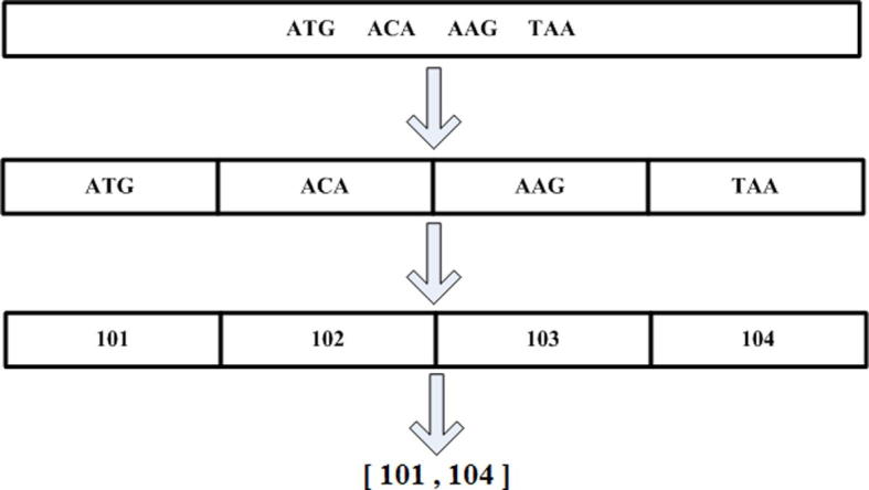
k-mer numbering, acting as a coding scheme, provides a compact representation of the k-mer paths. It is an assignment of a unique integer to each k-mer that appears in a DNA. If the same k-mer appears more than once, each instance must be assigned the same integer [27]. This simplification also helps in creating a database with entries (X, Y), where X are k-mer path intervals and Y are where they come from. This helps in the multiple local alignment (Figure 5) of all the reads identifying the k-mers that they share their orientation and location within them. This methodology is adapted from ARACHNE [13]. This further helps in making unipaths, as illustrated in Figure 5.

Figure 5.

Multiple local alignments (A) Spectrum: collection of all reads. (B) Collection of all k-mers derived from the reads. (C) The multiple alignment algorithms take a collection of unique k-mers. Then for each k-mer it does a local alignment with all the reads identifying the reads in which it is present, along with the starting position of the alignment within the read and also the orientation of its alignment. Using this, an overall alignment of the entire spectrum is obtained. (D) Unipath intervals: set of all k-mer path intervals. (E) Creating unipaths: take the first k-mer path interval, and its predecessor and concatenate it. Similarly take the last k-mer in the unipath, and its successor and concatenate it. Repeat iteratively this process to create unipaths. The unipath interval that is obtained using several k-mer path intervals in this example is [C, H]. (F) Branches: a branch in a graph is the point in the genome where there is a k-mer that appears in two or more places for which the next (or previous) bases are different. Here ([A, Z]), [A, H]) and ([Z, B], [H, B]) form a branch.

Building the graph

Multiple alignment and unipath generation pave the way for generating graphs which are then combined and cleaned up for the genome assembly. Most of the assemblers that rely on graph theory end up creating many graphs or contigs. These graphs could also be referred to as local assemblies whereas the complete graph obtained after scaffolding and graph simplification could be called the global assembly or the target genome.

After finding all minimal extensions and subsumptions for each read in the spectrum (see Supplementary section, [27]), local assembly is done by first finding all potential seeding unipaths. These seeds are found by filtering all unipaths that can be overlapped on either of its sides by other unipaths. The unipaths that remain are the seeders. The seed and 10 kb extension of genomic data on either side of the seed represents its neighbourhood. These seeds are extended, and their neighbourhood is built by making use of unipath intervals that define the most compact representation of individual unipaths. Assembling the neighbourhoods together yields the sequence graph whose edges are the unipaths.

These multiple local sequence graphs are connected to one another to form one global sequence graph which might have many parts, depending on the number of chromosomes in the genome or the success of the assembly process. The global assembly can be simplified or improved by (a) Disambiguation (Figure 3A), (b) Pulling-apart (Figure 3B) and (c) Clean-up, as depicted in (Figure 3I).

Velvet

Velvet [61] comes in line with all the other de novo assemblers that use de Bruijn graphs for genome assembly. The graph assembly process of Velvet is unique. Contrary to EULER where each node was a (k − 1) mer, a node N is a collection of overlapping k-mers that overlap by (k − 1) nucleotides, as shown in Figure 6. The complementary node of N and N^c is formed by the same process but using the reverse complements of these k-mers. N and N^c together form a block (Figure 6). Error correction is done via (a) removing tips (Figure 3I), and (b) removing bubbles (Figure 7).

Figure 6.

Velvet – making the database and the graph Velvet uses two databases (A) and (B) which are combined in a somewhat similar fashion to the database used by Allpaths in Figure 5. A hash table is used in (A) to store every k-mer, the ID of the first read encountered containing that k-mer and the start position of its occurrence within that read, and additionally its reverse complement. The second database (B) records, for each read which of its original k-mers are overlapped by other reads. Using (A) and (B), a third list of ordered original (unique) k-mers is made. The list is compartmentalized each time an overlap with another start or end occurs. The continuous set of reads in each compartment form the nodes of the graph in (C). Overlap between the last k-mers of one node and the first k-mer of the next node produces a directed edge (shown as yellow line) (C1). The blue lines represent the overlap of k-1 nucleotides between k-mers in the same node (C2). Furthermore, whenever an edge exists between a single parent N and its only child node then the two nodes are merged. This figure is adapted from [61].

Figure 7.

Velvet – removing bubbles As we progress along graph simplification, we see that shorter paths are being merged with longer paths. From (A) to (B), C is merged with C′ to form C′, and B is merged with B′ to form B. A similar process is repeated by merging B and B″ to form graph shown in panel (C) and finally panel (D). p-bubble fixing in EDENA is similar to that in Velvet. p-bubbles are branches caused by a single base substitution. Each branch is explored up to length δ. The length of the p-bubble is at most $\delta =4\times (\text{read length})-2\times (\text{minimum required overlap size})-1$. These are resolved by removing nodes on the less covered side of the bubble.

Scaffolding and repeat resolution are done using an inner module called Breadcrumb. It starts by identifying contigs longer than some threshold, called “long nodes”. These long nodes are then aligned and paired with other long nodes. This produces two sets of long nodes. One set contains long nodes that possibly connect with many at one end. They are ambiguous and left untouched. The other set contains only those long nodes that connect with only one other long node on either side of its ends. This set is then flagged and used for extension, taking one long node at a time and going as far as possible until it cannot be extended further by another flagged long node or it can have many plausible paired long nodes in which case one has ambiguity and plausible repeats. Contigs that are still ambiguously connected or branches in the graph that are still left unresolved are simplified by looking exhaustively at all plausible paths connecting two long nodes. This approach being cumbersome (since the search space is large), is reduced by identifying a sub-graph that only contains those nodes that are connected to two long contigs and leaving all the others. Now an exhaustive search reveals the true paths leading to one giant global assembly.

Edena: Exact de novo assembler

Edena [69] is another de novo graph-based assembler which follows the same processing schemes as all graph-based assemblers. In its filtering stage, reads that have ambiguities in base calling are discarded. Only one copy of the remaining reads is maintained, and the read and its reverse complement are considered to be the same. Therefore, paired-end data are not used in graph construction. However, the frequency of each read occurrence is kept for calculating depth of coverage.

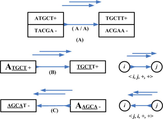
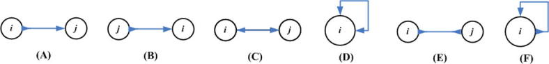
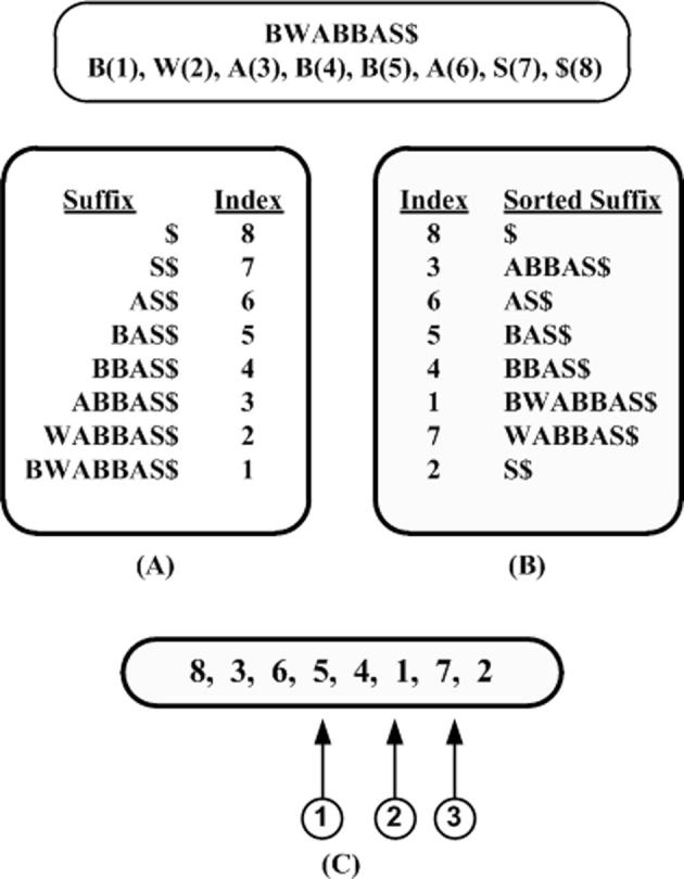
Edena’s graph construction uses suffix arrays [27], [70] for overlapping unique reads, where the minimum overlap size is determined heuristically. The structure is presented as a bidirectional graph structure [71], where each read corresponds to a node and an edge represents an overlap between two reads/nodes. Since the edges are bidirectional and the reads can be oriented in either way, so there are four possible ways to connect nodes.

Graph simplification is done by performing short dead-end path removal (Figure 3I), removing transitive edges (Figure 3K) and p-bubble fixing (Figure 7). After graph simplification, all contigs of minimum size that are unambiguously represented in the graph are provided as an output.

TAIPAN

TAIPAN [72], [73], simply put, is a graph-based approach where the contig extension is based on consensus. TAIPAN places the entire spectrum in a hash table which allows quick search of overlapping reads, which is then used to create a directed graph $\mathcal{G}$. For the consensus-based contig extension, two parameters k and T are taken, where k is the minimal overlap parameter and T is the contig length parameter. Any read can be considered as a seed and then extended. The seed is extended one base at a time, first from the 3′ end and then from the 5′ end. Once the graph has been constructed and the E₁ − E₂ – detachment resolved (Figure 3J), the remaining graph is used to evaluate the set of all vertex-disjoint paths P which help in contig extension. The seed is extended one base at a time if P has only one path whose length is greater than or equal to T. Then the first base in the path happens to be the extension of the seed. However, the seed is terminated in two cases. The first case occurs if there are insufficient overlapping reads, in which case the length of all paths in P is less than 1. The second case happens when there is a repeat in which case P has at least two paths whose lengths are greater than T and therefore the program cannot choose which path to extend. Reads that are used in the contig extension are removed from the hash table, thereby reducing the search space and speeding up the process.

Greedy approach

Greedy approach towards assembly of genomes is marked by three algorithms: short sequence assembly by progressive k-mer search and 3′ read extension (SSAKE) [74], verified consensus assembly by k-mer extension (VCAKE) [75] and quality-value-guided short read assembler (QSRA) [76] where each algorithm is an extension of the previous algorithm.

SSAKE proposed for assembly of genomes that were smaller is size (about 30 kb in length). SSAKE uses a hash table [27] and a prefix tree (see Supplementary section, [27]) to organize the read data along with its mate-pair information. The keys in hash table key are the reads and their associated values are the number of occurrences of the read. A consensus sequence is formed by placing in parallel all reads in such a manner that the prefix of a particular read matches the suffix of its predecessor read. This is done with the help of a prefix tree. Reads are composed of bases {A, C, G, T}. While searching for any particular read, each transition from parent to child divides the search space by four. If there are m reads, each of size n, then searching for a particular read is an O(n) or O(log₄ m) operation, since n steps are required from the root to reach the leaf. Every node shares common prefixes with its parents right up to the root node, which is a NULL node. The spectrum is organized by the prefixes of bases from their 5′ end. SSAKE requires coverage of 20× and a minimum base ratio of 0.6 to generate the contig [27], [74].

VCAKE [75] further improves upon the criterion of building and developing the contig by focusing on all reads that allow achieving a certain (coverage or overlap) depth t in order to achieve a good consensus of the seed. Seed is the term used sometimes to define the read or the contig which is being extended. In this regard, VCAKE has three user-defined measures (n, m, and e), each specifying the length of the overlap required with the 3′ end of the seed in decreasing level of strictness until a consensus depth of t is achieved. Each read that overlaps the seed is placed in the hash table with a value equal to the number of times it occurs. This process stops until a coverage depth of t occurs or a minimal overlap e is reached. Once the list of reads that generate the layout is identified then the extension proceeds one base at a time. A base is added from the consensus if it occurs more than c out of t times. However, if there is another base that exceeds $\mathcal{V}$ out of t times, the contig is terminated, plausibly suggesting a duplication of the sequence in another part of the genome. After this, all reads that were retrieved in the process and happen to occur completely within the contig are deleted both from the hash table and the prefix tree.

QSRA [76], further improves upon VCAKE by building and developing the contig by searching for reads whose bases overhang the overlap and have a Q_value > m, where m is a minimal user-defined Q_value score. It adds these reads in the consensus providing an overall larger average contig length. The extension continues until coverage t is obtained or no more reads are found whose overhanging bases have Q_values > m.

The contig is extended at the 3′ end by following the rules described above. Once all plausible extensions and all contigs are inferred then the complementary strand of the contig is considered to extend the contig on the 5′ end until all reads are exhausted.

Assisted assembly

Up until now, all the assemblers are categorized as being either comparative or de novo. Assisted assembly [77] lies between these two paradigms and, as such, adopts a de novo approach which relies on the assistance of the reference genome. It loosely adopts the alignment-overlap-layout-consensus scheme.

The reads are initially locally aligned to the reference genome (alignment phase). This helps to identify groups of reads that are eventually converted into contigs (overlap phase), as depicted in Figure 8. As far as the consensus phase is concerned, the contigs are created looking at both read alignment with the growing contig itself, and also alignment of the reads with the reference genome. In other words, even if the alignment of the read with the contig is not good, yet it aligns with the reference genome in close proximity to the contig then this is further evidence that the read belongs to the growing contig. This may appear to put some bias on the reference genome. However, the results of assisted assembly show overall good performance.

Figure 8.

Assisted assembly (A) The start/stop point of every read is inferred via local alignment with the reference genome. Reads are allowed to be placed more than once as well, in order to allow for duplicated regions within the genome. (B) If the start/stop positions of the reads overlap other reads by user-defined X number of bases, then the reads are grouped in one group. All such reads that overlap based on their positions in the reference genome form groups. (C) All groups are used to enlarge pre-existing contigs. If the group belongs to one contig, then that contig is enlarged (C1). If the group belongs to two contigs then the closest one is enlarged (C2). If a group does not belong to any contig, then the group itself becomes a new contig (C3). Once all the groups are dealt with, reads are taken from the groups one by one and are aligned with the contigs to extend them.

In the scaffolding phase, contigs are joined to one another via ‘trusted’ links. A link is trusted (or a pair of reads is valid) if its measure of stretch exceeds a user-defined threshold, i.e., it aligns to the reference genome uniquely and properly, and it also joins two scaffolds. Each read within the pair of reads that form this trusted link orients the scaffolds onto the reference genome in the same direction, and such reads are called ‘consistent’ reads. However, even if the link is not fully trusted, meaning its measure of stretch does not exceed the given threshold, yet all the conditions mentioned above are satisfied, in such cases the contigs are connected and scaffolding is done.

The scaffolding process may produce some chimeric scaffolds, whose ends belong to nonadjacent parts of the genome. Such scaffolds are identified as miss-assembled. These miss-assembled scaffolds are basically made up of reads that overlap one another to form consensus sequences. A search is conducted within these overlaps to look for such a consensus sequence that is backed up by just two reads overlapping with one another and not more than that. The point is that the miss-assembled scaffold, which is the weakest link, is broken up into two parts to form two contigs belonging to non-adjacent parts of the genome. After scaffolding, a series of de novo operations are done to simplify the graph in order to achieve global assembly.

A modular open-source comparative assembler (AMOS-Cmp)

AMOS is a collection of modules and libraries which are open-source and are useful in developing genome assemblers (http://www.sourceforge.net/apps/mediawiki/amos/index.php?title=AMOS). These AMOS modules, or stages, interact with one another via an AMOS data structure called “bank”.

AMOS-Cmp [78] uses the alignment-layout-consensus paradigm [27]. In the alignment stage, reads are aligned to the reference genome using maximal unique matching-mer (MUMmer, http://www.mummer.sourceforge.net) [79]. However, this alignment does not produce a unique alignment for every read along the reference genome. Some reads get aligned to more than one place along the genome and are called ‘repeats’. The reverse complements of the reads are used to resolve repeats, thereby aligning them to only one location on the reference sequence. The reverse complements of these repeats are also aligned with the reference genome. The location of the reverse complements aligned and that of the repeat is compared. If the distance is large, then those alignment locations are discarded. Furthermore, if the orientation (direction) of the alignment of the reverse complement and that of the repeats is not complementary, then that alignment location is also discarded. Otherwise, a random alignment amongst the plausible alignments for the repeat is chosen.

The alignment of all the reads produces a layout. Because the reads were derived from the novel (‘unknown’ or ‘target’) genome and were being aligned to a closely related reference genome, many reads might not align perfectly to the reference genome due to some mismatches, some insertions or deletions, or presence of some divergent areas (where the reference and the target genome differ greatly). These issues are resolved in a process called layout refinement, as illustrated in Figure 9. The divergent areas are resolved by generating the consensus sequence and then using that as a template for the alignment of the repeats. Layout refinement is repeated until the issues identified above are not faced anymore.

Figure 9.

AMOS-Cmp with layout refinement and gene boosted assembly Insertions in the reference (top left): (A) This is identified by reads aligned such that they span across the inserted area of the reference genome and align perfectly to either side of this inserted area. (B) In such case the ‘seeming gap’ is closed. (C) The genome surrounding the inserted area is considered as one contig. Insertions in the target sequence (top right): (D). This is identified by reads whose former portions align perfectly yet the latter portions diverge from the reference sequence. (E) This is resolved by breaking up the target genome at the point of insertion producing two contigs which are then (F) connected using the singletons of any assembly algorithm. Rearrangement (bottom right): regions 2 and 3 differ in their order and orientation from the reference and the target. Reads (G) and (H) match disjoint locations of the reference genome, shown as being connected via dashed lines. Insertions in the target sequence: this is resolved by breaking up the target genome at the point of insertion producing two contigs which are then connected using the singletons of any assembly algorithm. Figure was adapted from [78]. Gene boosted assembly (bottom left): contigs (A and B) form target 1, while contigs (C, D and E) form target 2. This method shows how two comparative assemblies can be used to close the gaps that occur in genome assembly. The target genome merges the contigs (A, B, C, D and E) to achieve the target genome. The shaded regions in the target genome and their corresponding location in the contigs show how this simple and elegant scheme works.

These steps provide a collection of contigs. Scaffolding uses mate-pair information. Two contigs can be considered to be adjacent to one another if two or more reads overlap the end of one contig and the start of the next. The stand-alone package used in AMOS-Cmp for scaffolding is Bambus [80]. Bambus allows any assembler to incorporate scaffolding in its assembly process by using it.

Gene boosted assembly (GBA) with short reads

GBA [81] is a comparative assembly approach that beautifully blends simple yet novel ideas with pre-existing tools to provide a solution. The method uses AMOS-Cmp, Minimus, Glimmer [82], Blast [83], assembly boosted by amino acids (ABBA, http://www.amos.sourceforge.net/docs/pipeline/abba.html), tblastn [84] and MUMmer [79] to achieve genome assembly of short reads. The simple yet novel idea is that instead of using one reference sequence for comparative assembly, two reference sequences are used to see how this helps the assembler performance.

Like all comparative schemes, GBA also uses the alignment-layout-consensus paradigm. Since GBA uses two reference sequences, the alignment of the reads with the reference sequence Ref₁ is done with the help of MUMmer, which is fine tuned to allow two mismatches in the alignment of every read with Ref₁. The results of the alignment are used to generate the initial target sequence target₁ by using AMOS-Cmp. GBA repeats the same process of using the reads, MUMmer and AMOS-Cmp to develop the target sequence target₂ only this time using the reference sequence Ref₂ as a template for assembly. The solution from the two assemblies target₁ and target₂ is compared to identify divergent areas of the target genome. This helps in filling in the gaps, using Minimus, and connecting the contigs in the right order, as depicted in Figure 9.

Gaps that are still left are filled up by using another simple yet novel approach of identifying protein-coding genes using Glimmer [82] and Blast [83]. Protein-coding genes are much more conserved than non-coding genes amongst genomes that belong to the same taxonomy or class. These predicted protein-coding sequences are used to align all the unused reads that were not used in building either target₁ or target₂, also called singletons in tblastn [84]. After alignment, these singletons help in filling up gaps and merging the contigs that surround these gaps using the algorithm called ABBA. Lastly, a de novo assembly of all the reads is done to produce newer contigs. MUMmer aligns these newer contigs with the contigs already present in order to fill up all the remaining gaps to produce the complete genome.

SHARCGS

SHARCGS stands for short-read assembler based on robust contig extension for genome sequencing [85]. SHARCGS is a de novo assembler which assumes a strong filtering of the reads to ensure that the assembly process generates contigs as large as possible. As a consequence of the filtering measures, the collection of contigs may not span the entire target genome. To avoid that, SHARCGS relaxes the filtering process in every iteration to include more and more reads in making the contig. A collection of contigs produced by different runs are merged together, by finding exact overlaps at least as long as one read length, to obtain the final assembly.

As a first step, SHARCGS in its pre-processing stage employs Q values for filtering data. Assuming that each base call in a read is independent of another, then the overall quality of a read of length r is P_correct = (1 − P_error)^r. SHARCGS uses this overall quality of the read to identify whether it should be used in the assembly process or discarded. If P_correct < q, where q is a user-defined parameter, then the reads are filtered out and not used in the assembly process. Even in the absence of Q values, a simple heuristic would be to count the number of times each read occurs; if it occurs at least n times then it is retained, otherelse discarded. The method used by SHARCGS to extend its contig is shown in Figure 10.

Figure 10.

SHARCGS for contig extension The shaded region in the contig to be extended is used as a prefix to gather all reads that share the same prefix. A prefix tree is employed for efficient search for all plausible reads having the same prefix. The ‘Extension’ region of the read “R” is the plausible extension sequence of the contig. To determine amongst all possible reads which one is to be used for extending the contig, a check sequence is employed “M”. This is made by combining the last ‘r’ bases of the extending contig and the extension region of R. Sub-strings of M are made and act as prefixes for searching other reads in the prefix tree. If all sub-strings retrieve one possible read whose prefix matches it, then the contig is extended, otherwise it is not.

Discussion

From Euler to Genovo [86], the mathematical and the algorithmic components of these assemblers were discussed. One simplistic extension to problem-solving would be to take ideas from previous assemblers, combine them and make an assembler with a performance overall better than the individual assemblers. New ideas may spring up by looking at papers that solve the jig-saw puzzle problem since genome assembly and the jig-saw puzzle are analogous to one another. This paper discussed extensively graph theory from the umbrella terms bidirected graphs and de Bruijn graphs (see Supplementary section, [27]), towards finding an optimal path such as the Hamiltonian path or the Eulerian path (see Supplementary section, [27]). The paper also discussed in detail algorithmic concepts like breadth-first search, prefix tree, suffix tree and suffix array (see Supplementary section, [27]). For the layman, details of the probabilistic distributions, Chinese restaurant process and maximum likelihood were also provided (see Supplementary section, [27]). In short, although the entire paper discussed in detail the NGS assemblers, both de novo and comparative schemes, nonetheless careful attention was given to concepts pertaining to probability theory, graph theory and algorithmic concepts so that the paper could be easily accessible to a wide audience.

After detailed discussion of the algorithmic components of various recipes to solve the genome assembler, it is extremely important to identify crucial aspects of scientific experimentation “reproducibility”, “accessibility”, and “computational transparency”. The sad facts are that the genome sequencing community is not very enthusiastic about reproducibility, accessibility and transparency [87]. Reproducibility of results published by genome analyses is a task that is tough and often hindered by many hurdles. Read data is one such hurdle since not all primary data is deposited in the Sequencing Read Archive (http://www.ncbi.nlm.nih.gov/sra). Other hurdles include absence of some tools or even presence of software tools in such conditions that installing them and making them work requires considerable expertise. As if things were not bad enough, the genomes published do not always provide all the details of which version of the assembler they used, and more importantly settings used by the assemblers in deriving the results. Therefore, people involved in making genome assemblers and the people who are using them should provide all the details in their papers to make their work more reproducible, accessible and transparent.

Still moving ahead, the realm of genome assembly requires a lot of improvement in terms of scalability of algorithms, especially when one is assembling a very large genome like that of human. One approach which is being explored is the use of Hadoop Mapreduce developed by Google [88]. Mapreduce is extremely scalable, efficient, reliable and runs on commodity computers. Genome analysis toolkit (GATK) is an alternative implementation for NGS but it is only parallel for one system, meaning that if a system presents 5 cores then it provides 5 parallel operations [89]. However, in its current format, it does not work on parallel systems. Use of Hadoop in genome assembly needs to be explored and is being explored by the community to exponentially speed up the assembly of large genomes [90]. However, time, effort and considerable expertise are required. Therefore, the realm of genome assembly is still very fresh in terms of algorithm development and it is still a place where one solution brings with it many open and complex questions. Also, since most of the genomes on the planet are yet to be sequenced, this is one area which will remain fresh for many years to come.

Competing interests

The authors have declared that no competing interests exist.

Supplementary material

Supplementary Figure 1.

Supplementary Figure 10.

Supplementary Figure 11.

Supplementary Figure 12.

Supplementary Figure 13.

Supplementary Figure 14.

Supplementary Figure 15.

Supplementary Figure 16.

Supplementary Figure 17.

Supplementary Figure 18.

Supplementary Figure 19.

Supplementary Figure 2.

Supplementary Figure 3.

Supplementary Figure 4.

Supplementary Figure 5.

Supplementary Figure 6.

Supplementary Figure 7.

Supplementary Figure 8.

Supplementary Figure 9.

References

- 1.Oxford Molecular Group PLC. AssemblyLIGN 1.0. 9. Oxford, United Kingdom: Oxford Molecular Group PLC; 1998.
- 2.Broveak T. Geneworks. Biotechnol Software Internet J. 1996;13:1114. [Google Scholar]
- 3.Parker S. Autoassembler sequence assembly software. Methods Mol Biol. 1997;70:107–118. doi: 10.1385/0-89603-358-9:107. [DOI] [PubMed] [Google Scholar]
- 4.Swindell S.R., Plasterer T.N. SEQMAN. Contig assembly. Methods Mol Biol. 1997;70:75–89. [PubMed] [Google Scholar]
- 5.Bromberg C. Gene Codes Corporation; 1995. Sequencher. [Google Scholar]
- 6.Miller S, Myers E. A fragment assembly project environment. University of Arizona, Dept. of Computer Science; 1991.
- 7.Gleeson T., Staden R. An x windows and unix implementation of our sequence analysis package. Comput Appl Biosci. 1991;7:398. doi: 10.1093/bioinformatics/7.3.398. [DOI] [PubMed] [Google Scholar]
- 8.Miller M.J., Powell J.I. A quantitative comparison of DNA sequence assembly programs. J Comput Biol. 1994;1:257–269. doi: 10.1089/cmb.1994.1.257. [DOI] [PubMed] [Google Scholar]
- 9.Sanger F. Nucleotide sequence of bacteriophage lambda DNA. J Mol Biol. 1982;162:729–773. doi: 10.1016/0022-2836(82)90546-0. [DOI] [PubMed] [Google Scholar]
- 10.Bastide M, McCombie WR. Assembling genomic DNA sequences with PHRAP. Curr Protoc Bioinformatics; 2007. [DOI] [PubMed]
- 11.Sutton G. Tigr assembler: a new tool for assembling large shotgun sequencing projects. Genome Sci Technol. 1995;1:919. [Google Scholar]
- 12.Myers E. A whole-genome assembly of drosophila. Science. 2000;287:2196–2204. doi: 10.1126/science.287.5461.2196. [DOI] [PubMed] [Google Scholar]
- 13.Batzoglou S. Arachne: a whole-genome shotgun assembler. Genome Res. 2002;12:177–189. doi: 10.1101/gr.208902. [DOI] [PMC free article] [PubMed] [Google Scholar]
- 14.Huang X., Madan A. Cap3: a DNA sequence assembly program. Genome Res. 1999;9:868–877. doi: 10.1101/gr.9.9.868. [DOI] [PMC free article] [PubMed] [Google Scholar]
- 15.Pop M. Genome sequence assembly: algorithms and issues. Computer. 2002:4754. [Google Scholar]
- 16.Streicher E.M. Spoligotype signatures in the mycobacterium tuberculosis complex. J Clin Microbiol. 2007;45:237–240. doi: 10.1128/JCM.01429-06. [DOI] [PMC free article] [PubMed] [Google Scholar]
- 17.Haddad N. Spoligotype diversity of mycobacterium bovis strains isolated in france from 1979 to 2000. J Clin Microbiol. 2001;39:3623–3632. doi: 10.1128/JCM.39.10.3623-3632.2001. [DOI] [PMC free article] [PubMed] [Google Scholar]
- 18.Sola C. Spoligotype database of mycobacterium tuberculosis: biogeographic distribution of shared types and epidemiologic and phylogenetic perspectives. Emerg Infect Dis. 2001;7:390–396. doi: 10.3201/eid0703.010304. [DOI] [PMC free article] [PubMed] [Google Scholar]
- 19.Duarte E.L. Spoligotype diversity of mycobacterium bovis and mycobacterium caprae animal isolates. Vet Microbiol. 2008;130:415–421. doi: 10.1016/j.vetmic.2008.02.012. [DOI] [PubMed] [Google Scholar]
- 20.Nivin B. Use of spoligotype analysis to detect laboratory cross-contamination. Infect Control Hosp Epidemiol. 2000;21:525–527. doi: 10.1086/501799. [DOI] [PubMed] [Google Scholar]
- 21.Voelkerding K. Next-generation sequencing: from basic research to diagnostics. Clin Chem. 2009;55:641–658. doi: 10.1373/clinchem.2008.112789. [DOI] [PubMed] [Google Scholar]
- 22.Mardis E. Next-generation dna sequencing methods. Annu Rev Genomics Hum Genet. 2008;9:387–402. doi: 10.1146/annurev.genom.9.081307.164359. [DOI] [PubMed] [Google Scholar]
- 23.Shendure J., Ji H. Next-generation DNA sequencing. Nat Biotechnol. 2008;26:1135–1145. doi: 10.1038/nbt1486. [DOI] [PubMed] [Google Scholar]
- 24.Schatz M. Assembly of large genomes using second-generation sequencing. Genome Res. 2010;20:1165–1173. doi: 10.1101/gr.101360.109. [DOI] [PMC free article] [PubMed] [Google Scholar]
- 25.Pop M. Genome assembly reborn: recent computational challenges. Brief Bioinform. 2009;10:354–366. doi: 10.1093/bib/bbp026. [DOI] [PMC free article] [PubMed] [Google Scholar]
- 26.Gormen TH et al. Introduction to algorithms, vol. 7. Chennai: MIT Press and McGraw-Hill Book Company; 1976. p. 1162–71.
- 27.Wajid B, Serpedin E. Supplementary information section: review of general algorithmic features for genome assemblers for next generation sequencers. <http://www.dl.dropbox.com/u/57205928/Appendix_Review_Paper_Bilal_Erchin.pdf>; 2011. [DOI] [PMC free article] [PubMed]
- 28.Nemhauser G.L., Wolsey L.A. vol. 18. Wiley; New York: 1998. (Integer and combinatorial optimization). [Google Scholar]
- 29.Papadimitriou C.H., Steiglitz K. Dover; 1998. Combinatorial optimization: algorithms and complexity. [Google Scholar]
- 30.Hromkovic J. Springer-Verlag; 2010. Algorithmics for hard problems: introduction to combinatorial optimization, randomization, approximation, and heuristics. [Google Scholar]
- 31.Korte B.H., Vygen J. vol. 21. Springer Verlag; 2006. (Combinatorial optimization: theory and algorithms). [Google Scholar]
- 32.Brouwer A.E., Haemers W.H. Springer Verlag; 2012. Spectra of graphs. [Google Scholar]
- 33.Stillman B. vol. 68. CSHL Press; 2003. (The genome of homo sapiens). [Google Scholar]
- 34.Rodriguez-Ezpeleta N. Springer Verlag; 2011. Bioinformatics for high throughput sequencing. [Google Scholar]
- 35.Padua D. Springer-Verlag; New York Inc: 2011. Encyclopedia of parallel computing. [Google Scholar]
- 36.Fleischner H. North-Holland; 1990. Eulerian graphs and related topics. [Google Scholar]
- 37.Myers E. Toward simplifying and accurately formulating fragment assembly. J Comput Biol. 1995;2:275–290. doi: 10.1089/cmb.1995.2.275. [DOI] [PubMed] [Google Scholar]
- 38.Miller J. Assembly algorithms for next-generation sequencing data. Genomics. 2010;95:315–327. doi: 10.1016/j.ygeno.2010.03.001. [DOI] [PMC free article] [PubMed] [Google Scholar]
- 39.Meader S. Genome assembly quality: assessment and improvement using the neutral indel model. Genome Res. 2010;20:675–684. doi: 10.1101/gr.096966.109. [DOI] [PMC free article] [PubMed] [Google Scholar]
- 40.Alkan C. Limitations of next-generation genome sequence assembly. Nat Methods. 2010;8:61–65. doi: 10.1038/nmeth.1527. [DOI] [PMC free article] [PubMed] [Google Scholar]
- 41.Koller D., Friedman N. The MIT Press; 2009. Probabilistic graphical models: principles and techniques. [Google Scholar]
- 42.Marcais G. Genome assembly, techniques; 2011.
- 43.Wendl M.C. Wiley; 2005. Genome assembly. Encyclopedia of genetics, genomics, proteomics and bioinformatics. [Google Scholar]
- 44.Koren S. An algorithm for automated closure during assembly. BMC Bioinformatics. 2010;11:457. doi: 10.1186/1471-2105-11-457. [DOI] [PMC free article] [PubMed] [Google Scholar]
- 45.Miller J.R. Aggressive assembly of pyrosequencing reads with mates. Bioinformatics. 2008;24:2818–2824. doi: 10.1093/bioinformatics/btn548. [DOI] [PMC free article] [PubMed] [Google Scholar]
- 46.Si J. vol. 2. Wiley-IEEE Press; Berlin: 2004. (Handbook of learning and approximate dynamic programming). [Google Scholar]
- 47.Lew A., Mauch H. vol. 38. Springer-Verlag; New York Inc: 2007. (Dynamic programming: a computational tool). [Google Scholar]
- 48.Denardo E.V. Dover Pubns; 2003. Dynamic programming: models and applications. [Google Scholar]
- 49.Sniedovich M. vol. 273. CRC; 2009. (Dynamic programming: foundations and principles). [Google Scholar]
- 50.Pevzner P. An Eulerian path approach to DNA fragment assembly. Proc Natl Acad Sci USA. 2001;98:9748–9753. doi: 10.1073/pnas.171285098. [DOI] [PMC free article] [PubMed] [Google Scholar]
- 51.Pevzner P. De novo repeat classification and fragment assembly. Genome Res. 2004;14:1786–1796. doi: 10.1101/gr.2395204. [DOI] [PMC free article] [PubMed] [Google Scholar]
- 52.Chaisson M., Pevzner P. Short read fragment assembly of bacterial genomes. Genome Res. 2008;18:324–330. doi: 10.1101/gr.7088808. [DOI] [PMC free article] [PubMed] [Google Scholar]
- 53.Chaisson M.J. De novo fragment assembly with short mate paired reads: does the read length matter? Genome Res. 2009;19:336–346. doi: 10.1101/gr.079053.108. [DOI] [PMC free article] [PubMed] [Google Scholar]
- 54.Raphael B. A novel method for multiple alignment of sequences with repeated and shuffled elements. Genome Res. 2004;14:2336–2346. doi: 10.1101/gr.2657504. [DOI] [PMC free article] [PubMed] [Google Scholar]
- 55.Medvedev P. Springer; 2007. Computability of models for sequence assembly. Algorithms in bioinformatics. Lecture Notes in Computer Science. p. 289–301. [Google Scholar]
- 56.Zhi D. Identifying repeat domains in large genomes. Genome Biol. 2006;7:R7. doi: 10.1186/gb-2006-7-1-r7. [DOI] [PMC free article] [PubMed] [Google Scholar]
- 57.McHugh JA. Algorithmic graph theory. Prentice Hall; 1990.
- 58.Kasianov V.N., Evstignee V.A. vol. 515. Springer; 2000. (Graph theory for programmers: algorithms for processing trees). [Google Scholar]
- 59.Cormen T.H. The MIT Press; 2001. Introduction to algorithms. [Google Scholar]
- 60.Gallier JH. Discrete mathematics, some notes. Technical reports (CIS); 2009. p. 897.
- 61.Zerbino D.R., Birney E. Velvet: algorithms for de novo short read assembly using de-bruijn graphs. Genome Res. 2008;18:821–829. doi: 10.1101/gr.074492.107. [DOI] [PMC free article] [PubMed] [Google Scholar]
- 62.Koffman E.B., Wolfgang P.A.T. Wiley; 2010. Data structures: abstraction and design using Java. [Google Scholar]
- 63.Dale N.B., Lewis J. Jones & Bartlett Learning; 2007. Computer science illuminated. [Google Scholar]
- 64.Neapolitan R.E., Naimipour K. Jones & Bartlett Learning; 2009. Foundations of algorithms. [Google Scholar]
- 65.Varghese G. Chapman & Hall/CRC; 2010. Network algorithmics. [Google Scholar]
- 66.Skiena S.S. vol. 1. Springer; 1998. (The algorithm design manual). [Google Scholar]
- 67.Butler J. Allpaths: de novo assembly of whole-genome shotgun microreads. Genome Res. 2008;18:810–820. doi: 10.1101/gr.7337908. [DOI] [PMC free article] [PubMed] [Google Scholar]
- 68.Gnerre S. High-quality draft assemblies of mammalian genomes from massively parallel sequence data. Proc Natl Acad Sci USA. 2011;108:1513–1518. doi: 10.1073/pnas.1017351108. [DOI] [PMC free article] [PubMed] [Google Scholar]
- 69.Hernandez D. De novo bacterial genome sequencing: millions of very short reads assembled on a desktop computer. Genome Res. 2008;18:802–809. doi: 10.1101/gr.072033.107. [DOI] [PMC free article] [PubMed] [Google Scholar]
- 70.Manber U., Myers G. Suffix arrays a new method for online string searches. SIAM J Sci Comput. 1993;22:935–948. [Google Scholar]
- 71.Myers E.W. The fragment assembly string graph. Bioinformatics. 2005;21(Suppl 2):ii79–ii85. doi: 10.1093/bioinformatics/bti1114. [DOI] [PubMed] [Google Scholar]
- 72.Schmidt B. A fast hybrid short read fragment assembly algorithm. Bioinformatics. 2009;25:2279–2280. doi: 10.1093/bioinformatics/btp374. [DOI] [PubMed] [Google Scholar]
- 73.Zhang W. A practical comparison of de novo genome assembly software tools for next-generation sequencing technologies. PLoS One. 2011;6:e17915. doi: 10.1371/journal.pone.0017915. [DOI] [PMC free article] [PubMed] [Google Scholar]
- 74.Warren R.L. Assembling millions of short dna sequences using ssake. Bioinformatics. 2007;23:500–501. doi: 10.1093/bioinformatics/btl629. [DOI] [PMC free article] [PubMed] [Google Scholar]
- 75.Jeck W.R. Extending assembly of short dna sequences to handle error. Bioinformatics. 2007;23:2942–2944. doi: 10.1093/bioinformatics/btm451. [DOI] [PubMed] [Google Scholar]
- 76.Bryant D.W. Qsra-a quality-value guided de novo short read assembler. BMC Bioinformatics. 2009;10:69. doi: 10.1186/1471-2105-10-69. [DOI] [PMC free article] [PubMed] [Google Scholar]
- 77.Gnerre S. Assisted assembly: how to improve a de novo genome assembly by using related species. Genome Biol. 2009;10:R88. doi: 10.1186/gb-2009-10-8-r88. [DOI] [PMC free article] [PubMed] [Google Scholar]
- 78.Pop M. Comparative genome assembly. Brief Bioinform. 2004;5:237–248. doi: 10.1093/bib/5.3.237. [DOI] [PubMed] [Google Scholar]
- 79.Kurtz S. Versatile and open software for comparing large genomes. Genome Biol. 2004;5:R12. doi: 10.1186/gb-2004-5-2-r12. [DOI] [PMC free article] [PubMed] [Google Scholar]
- 80.Pop M. Hierarchical scaffolding with bambus. Genome Res. 2004;14:149–159. doi: 10.1101/gr.1536204. [DOI] [PMC free article] [PubMed] [Google Scholar]
- 81.Salzberg S.L. Gene-boosted assembly of a novel bacterial genome from very short reads. PLoS Comput Biol. 2008;4:e1000186. doi: 10.1371/journal.pcbi.1000186. [DOI] [PMC free article] [PubMed] [Google Scholar]
- 82.Delcher A.L. Identifying bacterial genes and endosymbiont dna with glimmer. Bioinformatics. 2007;23:673–679. doi: 10.1093/bioinformatics/btm009. [DOI] [PMC free article] [PubMed] [Google Scholar]
- 83.Altschul S.F. Gapped blast and psi-blast: a new generation of protein database search programs. Nucleic Acids Res. 1997;25:3389–3402. doi: 10.1093/nar/25.17.3389. [DOI] [PMC free article] [PubMed] [Google Scholar]
- 84.Gertz E.M. Composition-based statistics and translated nucleotide searches: improving the tblastn module of blast. BMC Biol. 2006;4:41. doi: 10.1186/1741-7007-4-41. [DOI] [PMC free article] [PubMed] [Google Scholar]
- 85.Dohm J.C. Sharcgs, a fast and highly accurate short-read assembly algorithm for de novo genomic sequencing. Genome Res. 2007;17:1697–1706. doi: 10.1101/gr.6435207. [DOI] [PMC free article] [PubMed] [Google Scholar]
- 86.Laserson J., Jojic V., Koller D. Genovo: de novo assembly for metagenomes. J Comput Biol. 2011;18:429–443. doi: 10.1089/cmb.2010.0244. [DOI] [PubMed] [Google Scholar]
- 87.Goecks J. Galaxy: a comprehensive approach for supporting accessible, reproducible, and transparent computational research in the life sciences. Genome Biol. 2010;11:R86. doi: 10.1186/gb-2010-11-8-r86. [DOI] [PMC free article] [PubMed] [Google Scholar]
- 88.Lin J, Schatz M. Design patterns for efficient graph algorithms in mapreduce. In: Proceedings of the 8th workshop on mining and learning with graphs. ACM. p. 78–85.
- 89.McKenna A. The Genome Analysis Toolkit: a MapReduce framework for analyzing next-generation DNA sequencing data. Genome Res. 2010;20:1297–1303. doi: 10.1101/gr.107524.110. [DOI] [PMC free article] [PubMed] [Google Scholar]
- 90.Schatz M.C. Cloud computing and the DNA data race. Nat Biotechnol. 2010;28:691–693. doi: 10.1038/nbt0710-691. [DOI] [PMC free article] [PubMed] [Google Scholar]
Associated Data
This section collects any data citations, data availability statements, or supplementary materials included in this article.