Abstract
Ecosystem models often perform poorly in reproducing interannual variability in carbon and water fluxes, resulting in considerable uncertainty when estimating the land‐carbon sink. While many aggregated variables (growing season length, seasonal precipitation, or temperature) have been suggested as predictors for interannual variability in carbon fluxes, their explanatory power is limited and uncertainties remain as to their relative contributions. Recent results show that the annual count of hours where evapotranspiration (ET) is larger than its 95th percentile is strongly correlated with the annual variability of ET and gross primary production (GPP) in an ecosystem model. This suggests that the occurrence of favorable conditions has a strong influence on the annual carbon budget. Here we analyzed data from eight forest sites of the AmeriFlux network with at least 7 years of continuous measurements. We show that for ET and the carbon fluxes GPP, ecosystem respiration (RE), and net ecosystem production, counting the “most active hours/days” (i.e., hours/days when the flux exceeds a high percentile) correlates well with the respective annual sums, with correlation coefficients generally larger than 0.8. Phenological transitions have much weaker explanatory power. By exploiting the relationship between most active hours and interannual variability, we classify hours as most active or less active and largely explain interannual variability in ecosystem fluxes, particularly for GPP and RE. Our results suggest that a better understanding and modeling of the occurrence of large values in high‐frequency ecosystem fluxes will result in a better understanding of interannual variability of these fluxes.
Keywords: interannual variability, eddy covariance, ecosystem fluxes, short time scales
Key Points
Summing most active hours in carbon and water fluxes per year explains most of their interannual variability
Short‐term (hourly and daily) weather fluctuations strongly contribute to interannual variability in carbon and water fluxes
Understanding high values in ecosystem fluxes might help to constrain interannual variability in ecosystem models
1. Introduction
Terrestrial carbon and water fluxes are strongly influenced by fluctuations in climate. The terrestrial biosphere takes up about 25% of anthropogenic CO2 emissions, and interannual variations of the global net terrestrial carbon flux are the main driver of interannual variability of the growth rate of atmospheric CO2 [Le Quéré et al., 2015; Ahlström et al., 2015]. Terrestrial Biosphere Models (TBMs) are a primary tool for studying ecosystem fluxes and predicting how much carbon is taken up by the biosphere on an annual basis, yet understanding and predicting annual variations of ecosystem carbon and water fluxes is still challenging for these models [Fisher et al., 2014]. At both the site and global scale, the ability of TBMs to match observed interannual variability of carbon fluxes is limited [e.g., Keenan et al., 2012; Le Quéré et al., 2015].
In this contribution, we use the term interannual variability (IAV) to refer to the variability of the annual totals (sums over the year) of a given flux variable, generally ecosystem fluxes of carbon and water. At the site scale, a multitude of predictors have been suggested as main drivers of the IAV of carbon fluxes. These predictors include a combination of meteorological and vegetation descriptors, such as growing season precipitation, vapor pressure deficit, annual maximum of leaf area index, and growing season mean stomatal conductance [Stoy et al., 2006]; 2 year precipitation, mean annual temperature, and growing season length [Barr et al., 2007]; 3 year lagged water balance and annual potential evapotranspiration [Dunn et al., 2007]; moisture availability [Weber et al., 2009]; growing season length [Dragoni et al., 2011]; and autumn phenology, radiation, and soil water content [Wu et al., 2012a]. This list illustrates the great variety in drivers that have been associated with IAV of ecosystem fluxes and is by no means exhaustive.
As evident from the above list, aggregated variables at seasonal or annual scale are typically sought to predict annual ecosystem fluxes. Years can then be categorized into “dry” or “wet,” “hot” or “cold,” or even “favorable” and “unfavorable” for carbon uptake. However, for different sites or ecosystems, the set of variables explaining most of the IAV of ecosystem fluxes differs largely. This variability across sites hampers the derivation of a general set of rules for effective categorization of aggregate environmental conditions to improve the prediction of interannual variability in ecosystem fluxes.
Complementary to the research on long‐term aggregated environmental drivers, there is some evidence that short‐term variability (at the hourly scale) is important for IAV of ecosystem fluxes. For instance, Medvigy et al. [2010] found that short‐term variability in precipitation and radiation are good predictors for annual GPP using the Ecosystem Demography model version 2 (ED2). Paschalis et al. [2015] showed that short‐scale variability of meteorological drivers can affect water and carbon fluxes at the annual scale using the Tethys‐Chloris (T‐C) ecohydrological model [Fatichi et al., 2012]. Wu et al. [2012b] demonstrated that the sensitivity of carbon fluxes to meteorological variability is higher at shorter than at longer time scales in a beech forest.
Similar to the analysis of temporally aggregated drivers, these findings do not allow a derivation of general rules applicable for multiple sites or at the global scale. For this reason, here we search for relationships that can be generalized over different sites and ecosystems but still preserve a considerable information content, e.g., a high correlation with IAV. To this end, we focus on the distribution of observed hourly and daily carbon and water fluxes. More specifically, we examine characteristics of the distribution that explain a large fraction of the IAV and relate them to climatic drivers. Such insights shed light on the mechanisms controlling IAV, with a particular focus on short term versus long term and climatic versus phenological controls.
Recent work on GPP and ET has indicated that the tail ends of the distribution might drive most of the observed IAV. For data‐driven and modeled gridded GPP, a few positive and negative extreme anomalies that cover large spatial and temporal scales explain most of the spatially aggregated IAV of GPP. This is true for continental and global scales [Zscheischler et al., 2014a, 2014b]. Similarly, at the site‐level scale summing hours or days with high ET (exceeding the 95th percentile) is a good predictor for annual ET and GPP in an ecosystem model [Fatichi and Ivanov, 2014].
Here we use eddy covariance flux tower and weather data from eight temperate forest sites in the U.S. to investigate the short‐term controls of IAV on annual ecosystem fluxes. We specifically ask the following: (i) are the positive tails of GPP, RE, net ecosystem production (NEP), and ET (we will call them “most active hours” or “most active days”) strongly correlated with the annual sums in these variables? And if yes, (ii) are the most active hours and days related to climatic drivers and are these relationships similar for different sites? While model simulations suggest a positive answer to the first question [Fatichi and Ivanov, 2014], our study is novel in its reliance on observed site‐level data to explore these dynamics.
2. Data and Methods
2.1. Data
We used meteorological and eddy covariance data from eight towers of the AmeriFlux network (www.ameriflux.lbl.gov), all located in temperate forests in the U.S. (Figure 1 and Table 1). These data represent a subset of the synthesis data set described in Wolf et al. [2016], from which we extracted GPP, RE, NEP, ET, air temperature (T), precipitation (P), photosynthetically active radiation (PAR), and vapor pressure deficit (VPD) observations. Half‐hourly and hourly biosphere‐atmosphere fluxes of CO2, water vapor, and energy were processed using standardized procedures across sites according to established AmeriFlux standards [Boden et al., 2013]. Low turbulence conditions were filtered by using site specific friction‐velocity (u ∗) thresholds, as specified by the site Principle Investigators for each site. CO2 fluxes of NEP were partitioned into the component fluxes of GPP and RE with nighttime data (no photosynthesis), which was extrapolated to daytime using temperature response functions fit to moving bins within each year. Specific details on the flux partitioning and gap‐filling methods employed can be found in Wolf et al. [2016] and Barr et al. [2013]. Carbon uptake by the biosphere is denoted by positive NEP, while negative NEP indicates carbon losses to the atmosphere.
Figure 1.
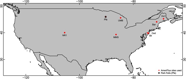
Map of the continental U.S. with the 8 AmeriFlux sites denoted by a red dot and their AmeriFlux site acronym. Park Falls (Pfa) is highlighted by a star.
Table 1.
AmeriFlux Sites Used in This Studya
| Site Name | Acronym | IGBP | Climate | Latitude | Longitude | MAT | MAP | Elevation | Years | Percentage of Missing Data | EBC | Reference |
|---|---|---|---|---|---|---|---|---|---|---|---|---|
| Bartlett | Bar | DBF | Dfb | 44.06 | −71.28 | 7.6 | 1303 | 272 | 2004–2012 | 48 | 0.71 | Jenkins et al. [2007] |
| Cedar Bridge | Ced | MF | Cfa | 39.83 | −74.37 | 12.3 | 1213 | 58 | 2006–2012 | 41 | 0.90 | Clark et al. [2014] |
| Howland Main | Ho1 | ENF | Dfb | 45.20 | −68.74 | 6.8 | 860 | 60 | 1996–2012 | 8 | 0.76 | Hollinger et al. [2004] |
| Morgan Monroe | MMS | DBF | Cfa | 39.32 | −86.41 | 12.5 | 1082 | 275 | 1999–2012 | 39 | 0.63 | Roman et al. [2015] |
| Niwot Ridge | NR1 | ENF | Dfc | 40.03 | −105.54 | 2.3 | 698 | 3050 | 1999–2012 | 11 | 0.74 | Monson et al. [2002] |
| Park Falls | Pfa | MF | Dfb | 45.94 | −90.27 | 6.0 | 577 | 470 | 1997–2012 | 23 | ‐ | Desai [2014] |
| Silas Little | Slt | DBF | Cfa | 39.91 | −74.59 | 12.6 | 1058 | 30 | 2005–2012 | 41 | 0.88 | Clark et al. [2014] |
| UMBS | UMB | DBF | Dfb | 45.55 | −84.71 | 7.4 | 870 | 234 | 2000–2012 | 39 | 0.76 | Gough et al. [2013] |
IGBP classes: DBF, Deciduous Broadleaf Forest; ENF, Evergreen Needleleaf Forest; and MF, Mixed Forest. Climate: Cfa, warm oceanic climate; Dfb, temperate continental climate; and Dfc, cool continental climate. MAT, mean annual temperature in °C; MAP, mean annual precipitation in mm/yr; percentage of missing data after quality assessment and quality control (QA/QC); EBC, energy balance closure computed as the slope of the regression of LE +H against R n−G at hourly scale.
Table 1 summarizes the key information about each site, including the dominant vegetation type (IGBP class), climate class, mean annual temperature (MAT), mean annual precipitation (MAP), and percentage of missing values. We further report the energy balance closure (EBC) as the slope of the regression L E + H against R n−G (LE = latent heat, H= sensible heat, R n= net radiation, and G= ground heat flux, if available), using ordinary least squares regression on all measured (nongap‐filled) hourly data. Park Falls has no measurements of net radiation; hence, the energy balance closure could not be computed.
2.2. Analysis
The distribution of ecosystem fluxes is generally largely positively skewed and long tailed; i.e., there are few occurrences with very high values (see Figure 2 for an example showing histograms of hourly GPP and NEP for Park Falls). Exploiting this property of high‐frequency flux data, we specifically focused on the positive tail of the distributions, as described in more detail in the following subsections.
Figure 2.
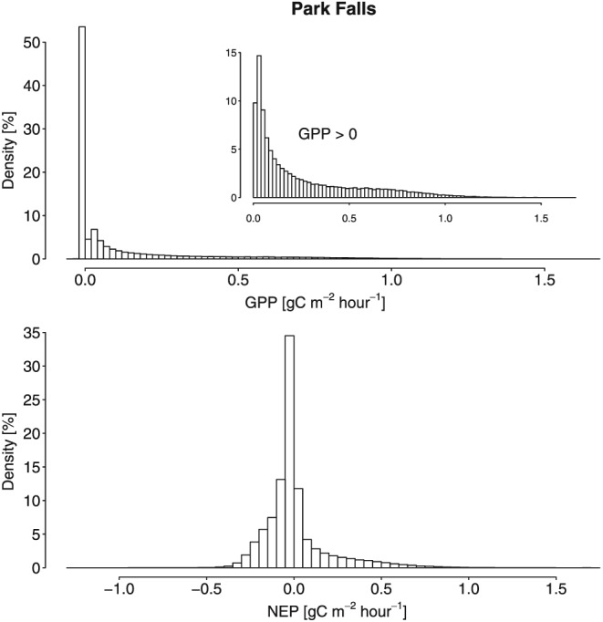
Histogram of hourly (top) GPP and (bottom) NEP at Park Falls (1997–2012). The y axis denotes the relative frequencies (in percent). The inset in the top shows histogram of all hourly GPP values greater than zero.
2.2.1. Most Active Hours and Days
For each of the fluxes GPP, RE, NEP, and ET, all percentiles 50%, 51%, …, 99% for hourly and daily fluxes were computed over the entire (≥7 years) time series (fluxes at lower percentiles of the distribution usually occurred in winter or at night). For each year, the number of hours/days that exceeded these percentiles was counted, and the resulting annual counts were correlated with the annual sums of the respective flux (equation (1)). For example, let x(y,i) be the hourly ecosystem flux of variable x with y = 1,…, number of years of observed data at the site and i be an hour in year y, we computed
| (1) |
where n is the number of hours in year y and p is the qth percentile of x computed over all years for q between 50 and 99. We call the resulting annual time series most active hours (MAH). In a similar fashion but using daily sums rather than hourly fluxes, we computed most active days (MAD). We computed time series of MAH and MAD for each ecosystem flux (GPP, RE, NEP, and ET) and each percentile. We then correlated each annual time series of MAH and MAD against the time series of the annual sums of their respective fluxes. For both temporal resolutions (hourly and daily), we computed the percentile where the average correlation over all eight sites reached its maximum. The best percentile for daily GPP (78th) and NEP (79th) at the Park Falls Ameriflux site in northern Wisconsin and the resulting linear relationship between annual fluxes and MAD are presented to illustrate the approach (Figure 3). Corresponding scatterplots for MAH are also shown for comparison (Figures 3c and 3f). Note that the percentile thresholds are different for the hourly scale (see Table 2).
Figure 3.
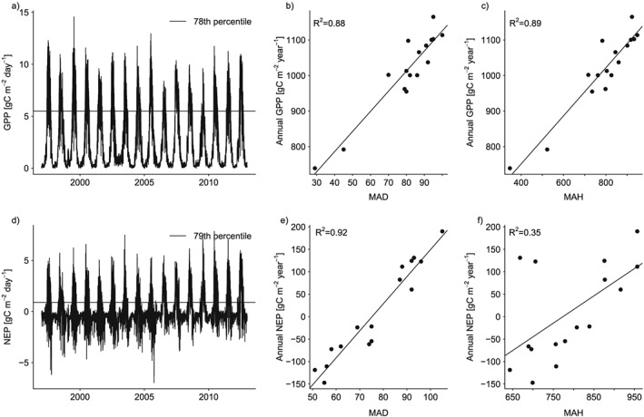
Illustration of the approach using daily (a) GPP and (d) NEP data at Park Falls. The horizontal lines denote the 78th and the 79th percentile for GPP and NEP, respectively. (b) Annual GPP versus number of days per year crossing the 78th percentile (i.e., MAD, see section 2.2.1). (c) For comparison: Annual GPP versus MAH. (e) Annual NEP versus number of days per year crossing the 79th percentile (MAD). (f) For comparison: Annual NEP versus MAH.
Table 2.
Optimal Percentile to Define MAH and MAD for Ecosystem Fluxes
| GPP | Reco | ET | NEP | |
|---|---|---|---|---|
| MAH | 91 | 74 | 90 | 91 |
| MAD | 78 | 73 | 82 | 79 |
We further investigated the extent to which the shape of the underlying data distribution determines the relationship between MAH and annual sums. To this end, we simulated hourly data for 50 years from the standard normal, gamma, and Pareto distribution. To simulate the effect that fluxes are zero (GPP and ET) or close to zero during winter and at night, we did an additional simulation with the Pareto distribution, randomly setting 50% of the hours to zero. The Pareto distribution is a heavy‐tailed distribution resembling most closely the properties of ecosystem flux data. We then computed MAH as explained above, repeated this 50 times, and report the average over these 50 simulations.
Finally, we assessed the importance of MAH and MAD for explaining the variability in annual totals in comparison to growing season length (GSL). We estimate spring and autumn phenological dates for each site year, based on smoothed daily integrated GPP. Spring and autumn phenological transitions were determined to be crossed when the GPP metric crossed a site‐specific threshold set to 10% of the 99th percentile of summer GPP values across all years at a site (following Keenan et al. [2014]). GSL was calculated as the difference between these two dates in days.
2.2.2. Estimate Importance of Drivers and Predict MAH
To estimate which climate drivers are most relevant for determining the most active hours and days in ecosystem fluxes, we performed a principal component analysis (PCA) on a set of drivers, projecting all drivers onto the first two principal components and noted whether most active hours occupied a distinct region of the plane delineated by the PCA axes when compared with the rest of hours. Taking basic ecophysiological processes [Bonan, 2008] and data availability into account, we selected the drivers day of the year, hour of the day, T, PAR, VPD, and cumulative P of the previous 30 days. Cumulative P of the previous 30 days was used as a proxy for water availability as soil water content was not available at all sites.
We further investigated whether a relationship between climatic drivers and the occurrence of most active hours can be established. Here we relied on Random Forests [Breiman, 2001], an ensemble machine‐learning method for classification. Random Forest is a statistical algorithm that is used to classify points of multidimensional data into different classes. We used Random Forests to classify hourly data into most active and other hours based on the same set of drivers as above. We used a random subset of 50% of the hours where NEP was observed (not gap filled) as training sample.
3. Results
Correlations between MAHGPP and annual GPP generally increase with increasing percentile up to a maximum around the 85th to 95th percentile before correlations decrease again (Figure 4). This behavior is most in line with simulations of a Pareto distribution where 50% of the hours were set to zero (Figure 5). MAH derived from normally distributed data reach the maximum correlation with annual sums at a much lower percentile. Correlations between MAH and annual sums from gamma‐distributed data are high up to approximately the 80th percentile before they decline rapidly. Correlations between MAHGPP and annual sums in observed data are considerably higher (correlation coefficients generally >0.85) than in simulated data, indicating that in the observed data distributions large values are even more strongly separated from the bulk of the distribution. The best percentile for defining MAH and MAD as a predictor for annual ecosystem fluxes varies between the 74th and 91st percentile for hourly fluxes and 73th and the 82th percentile for the daily fluxes (Table 2), with 91st and 78th percentiles giving the overall best performance for GPP at hourly and daily scale, respectively. That means, that counting the annual hours that exceed the 91st percentile correlates best with annual GPP.
Figure 4.
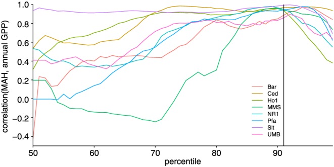
Correlation between annual sums of GPP and MAH for different percentiles used to define MAH. The vertical line indicates the percentile resulting in the highest correlation on average (91st). For the definition of MAH see section 2.2.1.
Figure 5.
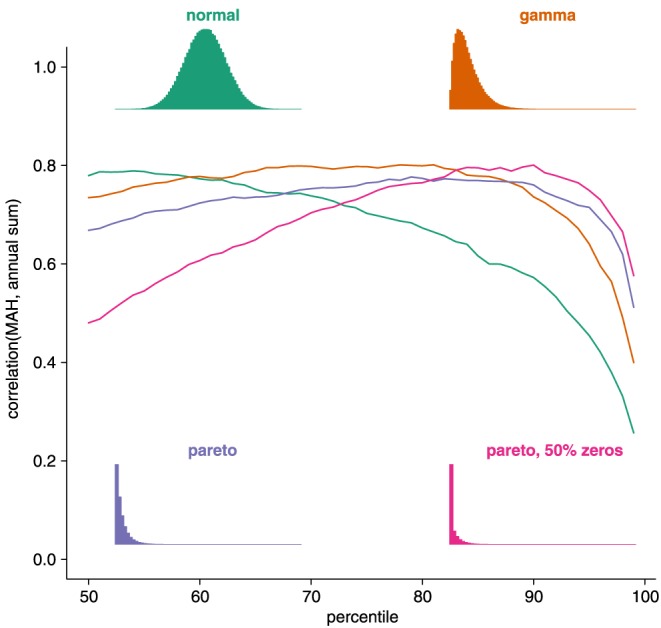
Correlation between MAH (see section 2.2.1) and annual sums for various percentiles and distributions based on simulated data. Fifty years of random hours are drawn from the following distributions: standard normal (green), gamma (orange), and Pareto (shape parameter equal to 10, blue). To simulate (close to) zero fluxes during winter and night another simulation with the Pareto distribution was conducted where 50% of the hours were set to zero (pink). Histograms of the distributions are shown as insets.
The relationship between the MAHGPP or MADGPP and annual GPP is very strong for all sites (Figure 6). For MAHGPP, the fraction of explained variance ranges between 74% (UMB) and 99% (Slt) with regression slopes between 0.61 gC m−2 yr−1 per most active hour for NR1 and 1.12 gC m−2 yr−1 per most active hour for UMB, (Figure 6a). For MADGPP, the fraction of explained variance is in a similar range (between 71% for Ho1 and 99% for Slt). Regression slopes vary between 2.92 (NR1) and 9.32 gC m−2 yr−1 per most active day (Slt). Note that forests in Slt were largely defoliated by the Gypsy moth in 2007, resulting in very low annual GPP and NEP [Clark et al., 2010], and low MAH and MAD. Because regression slopes vary between sites, a unique linear model to encompass the relationship between MAHGPP or MADGPP and annual GPP for all sites cannot be expected. No relationship between the regression slopes and climatic drivers could be found.
Figure 6.
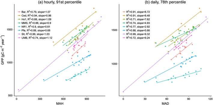
Annual GPP versus number of (a) MAH and (b) MAD (see section 2.2.1). The resulting fraction of explained variance (R 2) and the resulting slopes are given in the legend. Site acronyms as in Table 1.
Figure 7 summarizes the strengths of relationship between MAH, MAD, GSL, and IAV for all sites and all variables. In summary, it describes how much of the variance in annual sums is explained by MAH, MAD, and GSL. Overall, MAD and MAH explain large fractions of the IAV in ecosystem fluxes, and there is little difference between sites and temporal resolutions except for NEP. For NEP, the relationship at daily resolution is much stronger for some sites (MAD is a better predictor than MAH). This is probably due to the gap‐filling scheme used which introduces some uncertainties in the annual values of NEP depending on whether hourly or daily values are aggregated [Wolf et al., 2016]. In contrast, the explanatory power of GSL is much lower. For GPP on average, MAH and MAD explain more than twice as much variability than GSL, for the other variables the difference is even larger.
Figure 7.
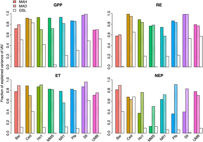
Fraction of explained variance of annual sums of carbon and water fluxes by most active hours (MAH, colored bars), most active days (MAD, striped bars), and growing season length (GSL, white bars). For the definition of MAH, MAD, and GSL see section 2.2.1.
A principal component analysis (PCA) of hourly climate data of Park Falls shows the separation between “most active” and “other” hours (Figure 8). Climatic drivers are projected onto the first two principal components, explaining nearly 74% of the variance in the drivers. The distributions of most active hours and the remaining hours are quite well separated, mostly by high VPD and high PAR. For RE, most active hours are better separated in the direction of high temperature, high 30 day precipitation, and day of the year (Figure 8b). Despite the overall good separation, some hours seem to fulfill the general climatic conditions for being most active hours but are in fact not (red dots in the blue point clouds in Figure 8). The relationships look qualitatively very similar for the other sites (not shown). The first principal component explains between 44.6 and 49.2% of the variance, the second principal component between 21.8 and 24.6%. In all sites, MAH in GPP, NEP, and ET are separated mostly along the direction of high PAR and VPD, and MAH in RE are separated mostly along high P (30d), T, and the day of the year.
Figure 8.
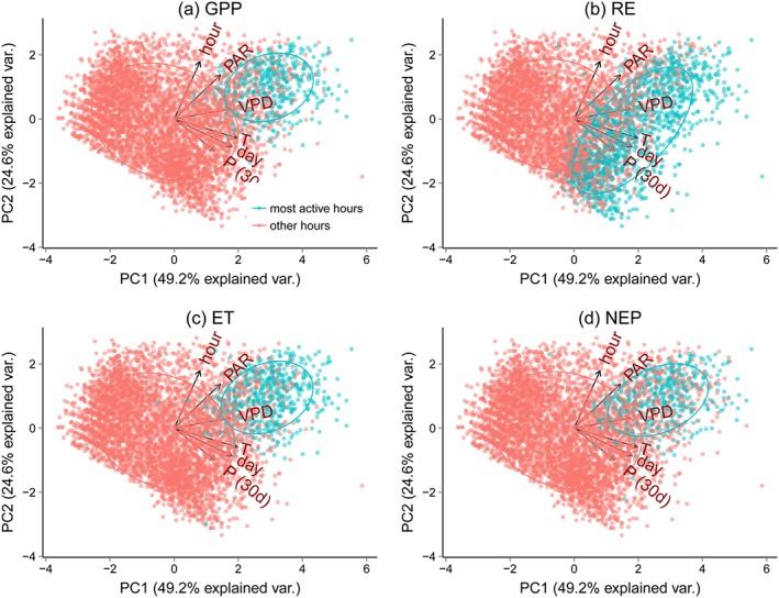
Principal component analysis for driving data for Park Falls, projection on the first two principal components (PC). MAH are marked blue (see section 2.2.1). VPD, vapor pressure deficit; PAR, photosynthetically active radiation; P(30d), cumulative precipitation over the last 30 days; hour, hour of the day; and day, day of the year.
We classified hourly data into MAH and other hours from climate variables using Random Forests and compare the number of hours classified as MAH with the annual fluxes. We do this for all four fluxes and use again Park Falls as an example to illustrate the results (Figure 9). MAHGPP and MAHRE can be classified relatively well, and consequently, the number of predicted MAH is a good indicator for the annual GPP and RE fluxes (R2= 0.92 and 0.82, respectively). For ET the prediction skill is a bit weaker (R2= 0.68), and it is low for NEP (R2= 0.12). Similar patterns are found at the other sites, with averaged R2 of 0.62, 0.8, 0.47, and 0.36 for GPP, RE, ET, and NEP, respectively. The prediction undertaken here is left intentionally simple (only a few driving variables are used, and no lagged effects are incorporated) and merely serves the purpose to illustrate that a prediction of MAH from climate drivers is possible through binary classification, particularly for GPP and RE.
Figure 9.
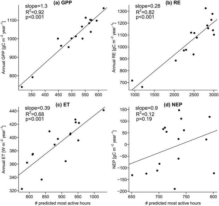
Annual carbon and water fluxes versus predicted MAH for Park Falls (see section 2.2.1). The following predictors were used for the binary classification to predict whether an hour is most active or not: day of the year, hour of the day, T, PAR, VPD, and cumulative precipitation over the last 30 days.
4. Discussion
We have shown that the sum of hours or days where ecosystem fluxes are large (exceeding a high percentile) is linearly related to the annual sum of this ecosystem flux using observed flux data, which answers our first research question. Such a relationship was previously found using simulations from an ecosystem model [Fatichi and Ivanov, 2014], but in that work it was not possible to confidently conclude that this relationship was not somehow influenced by the model structure. Our results based on measured data from eight sites (96 site years) demonstrate that this is indeed a relevant phenomenon and not an artifact of model structure. Our analysis of artificial data suggests that the relationship is strongly driven by the shape of the distribution of ecosystem fluxes. Additionally, part of the relationship between MAH/MAD and annual sums can probably be explained through spurious self‐correlation because all involved variables are derived from the same single variable [Kenney, 1982]. However, given that the relationships are very strong and that MAH separate the driver space fairly well (Figure 8), it can be expected that there is an underlying mechanism leading to MAH which then in turn shape the annual sums. This addresses the second question presented in the introduction, namely, whether the positive tails of ecosystem fluxes can be related to climatic drivers. As we demonstrated the MAH are generally related to similar short‐term weather conditions, largely driven by variations in VPD and PAR (GPP, NEP, and ET), as well as T, 30 day precipitation, and day of the year (RE). We further discuss whether these short‐term “favorable conditions” are really an important and poorly predictable component in determining the annual sums or whether they are for instance just resulting from seasonally averaged climate variables.
4.1. On the Temporal Distribution of Most Active Hours
If seasonally aggregated climate drivers dominate the annual sums of ecosystem fluxes, one would expect the occurrence of MAH to be easily predictable along the course of the year, for example, forming a clear pattern during the growing season. In this case, it could be expected that during the growing season the number of most active hours should vary little between days. However, as Figure 10 suggests, the number of most active hours on a given day exhibits relatively complex and varying patterns for different years. Some predictability on the synoptic scale can be expected, as the autocorrelation usually falls below the significance level (95%) only after 1 or 2 weeks. The number of most active hours per day is generally higher during years with higher annual GPP, yet the shape of the distribution of number of most active hours varies largely for different years (Figure 10). This suggests that a most active hour requires that slowly evolving variables like soil moisture (at least in the depletion phase) and leaf area index be high and that meteorological variables that change over synoptic and shorter time scales (like radiation, temperature, and VPD) are concurrently favorable. The combination of these long‐term predisposing factors with short‐term favorable meteorological drivers then define the annual sums of ecosystem fluxes and their variability across years. For instance, very favorable meteorological drivers will not lead to a most active hour if the ecosystem has a low leaf area index because the canopy is developing or senescing or the ecosystem is still recovering from a previous drought or an early season frost. Moreover, the combination of different meteorological drivers may be necessary at certain sites for a most active hour to occur even in the presence of an overall positive situation, being PAR, VPD, and temperature important but not the only controls. This is underlined by the observation that growing season length is a much weaker predictor for IAV (Figure 7) though the range of occurrences of MAH is well captured by the GSL (Figure 10). MAH and MAD are much more flexible and can capture unfavorable weather conditions even after the canopy is fully developed. Such conditions in turn can have a profound impact on the annual totals.
Figure 10.
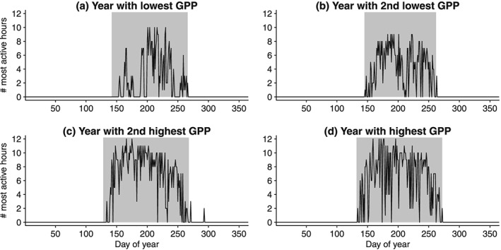
Number of most active hours per days for the year with (a) lowest, (b) second lowest, (c) second highest, and (d) highest GPP at Park Falls. Grey shading indicates the growing season.
Sometimes, an hour is not classified as a most active hour even when it is characterized by short‐term conditions that are typical for the MAHs (Figure 8). This could be due to several factors including nonlinear dependencies and cross correlation between climatic drivers and the occurrence of MAH (for instance, lagged effects) or missing relevant drivers to separate the two. Noise in the data can also contribute [Hollinger and Richardson, 2005] but since similar results are obtained from model simulations [Fatichi and Ivanov, 2014] is unlikely to represent a major issue. While the overall impact of seasonally favorable climate conditions on carbon fluxes might be comparatively easy to predict (though variable across sites), the effects of short‐term weather variations probably represent a more significant challenge.
4.2. Implications for Modeling and Predictability
We have shown that the occurrence of MAH can be predicted relatively well for GPP, RE, and ET with hourly‐scale climatic drivers (Figure 9). MAH in NEP are harder to predict, probably because the initial relationship between MAH and NEP is weak (Figures 3 and 7). Moreover, NEP is the difference between two large fluxes such that it integrates more complex processes and is also subjected to larger uncertainties. MAHNEP are also more difficult to separate with the small subset of drivers which we used here (Figure 8).
If IAV of ecosystem fluxes is to be captured well with mechanistic models, climatic drivers need to be available locally at high temporal resolution and of very good quality, and models need to be well calibrated with a precise representation of the current ecosystem state to accurately translate short‐term weather variability into changes in ecosystem fluxes. Recognizing that capturing the positive tails of the data distribution is important could also improve the calibration of mechanistic models and cost‐function definitions. In particular, for calibrating model parameters one could give more weight to errors in high values rather than considering every hour with the same weight. This is likely to improve model performance with respect to IAV and could also be important for model‐data integration studies [Raupach et al., 2005; Dietze et al., 2013; Keenan et al., 2013; Niu et al., 2014]. At the same time, large values are often accompanied with larger uncertainties, impeding a straightforward translation of our results into cost functions. Alternatively, cost functions may be based on the occurrence of MAH rather than on the exact flux values. As a side result, our findings indicate that predictive ability for IAV of ecosystem models using seasonal or monthly forcing only will be limited. At the hourly and daily time scale, the relationship between most active periods and IAV is similarly strong, suggesting that running models at daily time steps might be enough to capture IAV well. However, due to nonlinearities in ecosystem response to radiation, VPD, temperature, etc., matching the most active days well likely requires models to be very accurate on the hourly time step as well.
The above observations are consistent with a recent study based on a mechanistic model demonstrating that short‐scale variability of meteorological input does affect water and carbon fluxes across a wide range of time scales, spanning from the hourly to the annual and longer scales, especially when the information content of meteorological inputs can be integrated in time, for instance, through soil moisture effects [Paschalis et al., 2015]. The study also showed that different ecosystems respond to characteristics of short‐scale variability of the climate forcing in various ways depending on dominant factors limiting ecosystem productivity, which renders a generalization quite challenging.
The importance of extreme values in GPP for its IAV has been shown before at the site‐level [Wei et al., 2014], continental [Zscheischler et al., 2014a], and global scales [Zscheischler et al., 2014b]. While those studies are also mostly based on the distribution of GPP values, droughts could be identified as the major driver for large‐scale negative anomalies in GPP. IAV in ecosystem fluxes measured by the eddy covariance technique has been extensively studied [Stoy et al., 2006; Barr et al., 2007; Dunn et al., 2007; Keenan et al., 2012], yet results are still difficult to generalize. This could be attributed to issues of data quality, but it is more likely that the complexity of the problem requires longer observations. Eddy covariance observations are mostly shorter than 20 years, and generalizable results are difficult to obtain from such short time series. Nevertheless, studying the underlying data distributions offers alternative avenues of research and can result in new insights. Our results suggest that focusing research on understanding the occurrence of high flux values (beyond the 75th–90th percentile) might also result in a better understanding of the IAV in ecosystem fluxes.
Lagged responses to climate anomalies can strongly affect ecosystem fluxes [Bréda et al., 2006; Bigler et al., 2007; Arnone et al., 2008; Goebel et al., 2011] and are neglected in this study. In particular climate extremes can have notable impacts on ecosystem fluxes [Reichstein et al., 2013; Frank et al., 2015]. Climate projections of mean or seasonal changes are relatively robust; however, there is less confidence on the capability of climate models to simulate changes in short‐term meteorological variability and extremes [Seneviratne et al., 2012]. Changes in climate extremes might strongly influence the occurrence of MAH and thus induce changes in the IAV of ecosystem fluxes.
We do not expect, however, that the relationship between MAH and carbon and water fluxes will drastically change with a change in variability. After all, the distribution of MAH is shaped by climate anomalies and extremes. Events with strong impacts on vegetation lead to low MAH and MAD, and low GPP, as the example of the attack of the Gypsy moth in 2007 in Slt demonstrates (Figure 6). Similarly, these relationships are expected to hold in other ecosystems than temperate forests. As a previous modeling study shows, MAH and GPP are strongly related in a semiarid shrub ecosystem and a seasonally dry grassland [Fatichi and Ivanov, 2014]. We speculate that this statistical relationship holds particularly well in semiarid ecosystems, where drier years lead to lower MAH and carbon uptake whereas wetter years are expected to have higher MAH and carbon uptake. In such ecosystems, large flux values might be well separated from the bulk of the distribution, rendering a prediction of MAH easier. In contrast, in tropical forests these relationships might not be as strong if fluxes show an overall lower interannual variability and thus less heavy tailed distributions.
5. Conclusion
We have shown that the number of occurrences of high values in observed hourly and daily ecosystem fluxes (GPP, RE, NEP, and ET) are strongly correlated with their annual sums, while the influence of phenological transitions had less importance. These most active hours and days cover a small part of the data distribution (typically less than 20%) but shape the annual fluxes to a large extent. The most active hours can be relatively well separated in the case of GPP and RE and thus be predicted by environmental drivers. The relationship between most active hours and IAV in ecosystem fluxes is demonstrated for temperate forests; however, since it is mostly a property of the high‐frequency flux distribution, we assume that this relationship also holds for other ecosystems. Our results indicate that annual values of ecosystem fluxes are driven by a combination of long‐term predisposing climatic and biological factors and short‐term favourable weather conditions. They further suggest that if the occurrence of the most active hours in ecosystem fluxes can be well understood and modeled, this could contribute to a better understanding of the IAV in these fluxes.
Acknowledgments
The AmeriFlux sites US‐MMS and US‐NR1 are currently supported by the U.S. Department of Energy, Office of Science, through the AmeriFlux Management Project (AMP) at Lawrence Berkeley National Laboratory under award 7094866. We thank Andrew Richardson for providing the data of Bartlett Experimental Forest. S.F. thanks the Stavros Niarchos Foundation and the ETH Zurich Foundation (grant ETH‐29 14‐2) for their support. S.W. was supported by the European Commission with a Marie Curie International Outgoing Fellowship (grant 300083). All used data are available from the AmeriFlux network (www.ameriflux.lbl.gov).
Zscheischler, J. , et al. (2016), Short‐term favorable weather conditions are an important control of interannual variability in carbon and water fluxes, J. Geophys. Res. Biogeosci., 121, 2186–2198, doi:10.1002/2016JG003503.
References
- Ahlström, A. , et al. (2015), The dominant role of semi‐arid ecosystems in the trend and variability of the land CO2 sink, Science, 348(6237), 895–899, doi:10.1126/science.aaa1668. [DOI] [PubMed] [Google Scholar]
- Arnone, J. A. , et al. (2008), Prolonged suppression of ecosystem carbon dioxide uptake after an anomalously warm year, Nature, 455(7211), 383–386. [DOI] [PubMed] [Google Scholar]
- Barr, A. , et al. (2013), Use of change‐point detection for friction–velocity threshold evaluation in eddy‐covariance studies, Agric. For. Meteorol., 171, 31–45. [Google Scholar]
- Barr, A. G. , Black T., Hogg E., Griffis T., Morgenstern K., Kljun N., Theede A., and Nesic Z. (2007), Climatic controls on the carbon and water balances of a boreal aspen forest, 1994–2003, Global Change Biol., 13(3), 561–576. [Google Scholar]
- Bigler, C. , Gavin D. G., Gunning C., and Veblen T. T. (2007), Drought induces lagged tree mortality in a subalpine forest in the Rocky Mountains, Oikos, 116(12), 1983–1994. [Google Scholar]
- Boden, T. A. , Krassovski M., and Yang B. (2013), The AmeriFlux data activity and data system: An evolving collection of data management techniques, tools, products and services, Geosci. Instrum. Methods Data Syst., 2(1), 165–176. [Google Scholar]
- Bonan, G. (2008), Ecological Climatology: Concepts and Applications, Cambridge Univ. Press, Cambridge, U. K. [Google Scholar]
- Bréda, N. , Huc R., Granier A., and Dreyer E. (2006), Temperate forest trees and stands under severe drought: A review of ecophysiological responses, adaptation processes and long‐term consequences, Ann. For. Sci., 63, 625–644. [Google Scholar]
- Breiman, L. (2001), Random forests, Mach. Learn., 45(1), 5–32. [Google Scholar]
- Clark, K. , Skowronski N., Gallagher M., Renninger H., and Schäfer K. (2014), Contrasting effects of invasive insects and fire on ecosystem water use efficiency, Biogeosciences, 11(23), 6509–6523. [Google Scholar]
- Clark, K. L. , Skowronski N., and Hom J. (2010), Invasive insects impact forest carbon dynamics, Global Change Biol., 16(1), 88–101, doi:10.1111/j.1365-2486.2009.01983.x. [Google Scholar]
- Desai, A. R. (2014), Influence and predictive capacity of climate anomalies on daily to decadal extremes in canopy photosynthesis, Photosynth. Res., 119(1–2), 31–47. [DOI] [PubMed] [Google Scholar]
- Dietze, M. C. , Lebauer D. S., and Kooper R. (2013), On improving the communication between models and data, Plant Cell Environ., 36(9), 1575–1585. [DOI] [PubMed] [Google Scholar]
- Dragoni, D. , Schmid H. P., Wayson C. A., Potter H., Grimmond C. S. B., and Randolph J. C. (2011), Evidence of increased net ecosystem productivity associated with a longer vegetated season in a deciduous forest in south‐central Indiana, USA, Global Change Biol., 17(2), 886–897. [Google Scholar]
- Dunn, A. L. , Barford C. C., Wofsy S. C., Goulden M. L., and Daube B. C. (2007), A long‐term record of carbon exchange in a boreal black spruce forest: Means, responses to interannual variability, and decadal trends, Global Change Biol., 13(3), 577–590. [Google Scholar]
- Fatichi, S. , and Ivanov V. Y. (2014), Interannual variability of evapotranspiration and vegetation productivity, Water Resour. Res., 50, 3275–3294, doi:10.1002/2013WR015044. [Google Scholar]
- Fatichi, S. , Ivanov V., and Caporali E. (2012), A mechanistic ecohydrological model to investigate complex interactions in cold and warm water‐controlled environments: 1. Theoretical framework and plot‐scale analysis, J. Adv. Model. Earth Syst., 4, M05002, doi:10.1029/2011MS000086. [Google Scholar]
- Fisher, J. B. , Huntzinger D. N., Schwalm C. R., and Sitch S. (2014), Modeling the terrestrial biosphere, Annu. Rev. Environ. Resour., 39, 91–123. [Google Scholar]
- Frank, D. , et al. (2015), Effects of climate extremes on the terrestrial carbon cycle: Concepts, processes and potential future impacts, Global Change Biol., 21, 2861–2880, doi:10.1111/gcb.12916. [DOI] [PMC free article] [PubMed] [Google Scholar]
- Goebel, M. O. , Bachmann J., Reichstein M., Janssens I. A., and Guggenberger G. (2011), Soil water repellency and its implications for organic matter decomposition—Is there a link to extreme climatic events?, Global Change Biol., 17(8), 2640–2656. [Google Scholar]
- Gough, C. M. , Hardiman B. S., Nave L. E., Bohrer G., Maurer K. D., Vogel C. S., Nadelhoffer K. J., and Curtis P. S. (2013), Sustained carbon uptake and storage following moderate disturbance in a Great Lakes forest, Ecol. Appl., 23(5), 1202–1215. [DOI] [PubMed] [Google Scholar]
- Hollinger, D. , and Richardson A. (2005), Uncertainty in eddy covariance measurements and its application to physiological models, Tree Physiol., 25(7), 873–885. [DOI] [PubMed] [Google Scholar]
- Hollinger, D. Y. , et al. (2004), Spatial and temporal variability in forest–atmosphere CO2 exchange, Global Change Biol., 10(10), 1689–1706. [Google Scholar]
- Jenkins, J. , Richardson A., Braswell B., Ollinger S., Hollinger D., and Smith M.‐L. (2007), Refining light‐use efficiency calculations for a deciduous forest canopy using simultaneous tower‐based carbon flux and radiometric measurements, Agric. For. Meteorol., 143(1), 64–79. [Google Scholar]
- Keenan, T. , et al. (2012), Terrestrial biosphere model performance for inter‐annual variability of land‐atmosphere CO2 exchange, Global Change Biol., 18(6), 1971–1987. [Google Scholar]
- Keenan, T. F. , Davidson E. A., Munger J. W., and Richardson A. D. (2013), Rate my data: Quantifying the value of ecological data for the development of models of the terrestrial carbon cycle, Ecol. Appl., 23(1), 273–286. [DOI] [PubMed] [Google Scholar]
- Keenan, T. F. , et al. (2014), Net carbon uptake has increased through warming‐induced changes in temperate forest phenology, Nat. Clim. Change, 4(7), 598–604. [Google Scholar]
- Kenney, B. C. (1982), Beware of spurious self‐correlations!, Water Resour. Res., 18(4), 1041–1048. [Google Scholar]
- Le Quéré, C. , et al. (2015), Global carbon budget 2014, Earth Syst. Sci. Data, 7(1), 47–85. [Google Scholar]
- Medvigy, D. , Wofsy S. C., Munger J. W., and Moorcroft P. R. (2010), Responses of terrestrial ecosystems and carbon budgets to current and future environmental variability, Proc. Natl. Acad. Sci. U.S.A., 107(18), 8275–8280. [DOI] [PMC free article] [PubMed] [Google Scholar]
- Monson, R. , Turnipseed A., Sparks J., Harley P., Scott‐Denton L., Sparks K., and Huxman T. (2002), Carbon sequestration in a high‐elevation, subalpine forest, Global Change Biol., 8(5), 459–478. [Google Scholar]
- Niu, S. , Luo Y., Dietze M. C., Keenan T. F., Shi Z., Li J., and Chapin F. S. III (2014), The role of data assimilation in predictive ecology, Ecosphere, 5(5), 1–16. [Google Scholar]
- Paschalis, A. , Fatichi S., Katul G. G., and Ivanov V. Y. (2015), Cross‐scale impact of climate temporal variability on ecosystem water and carbon fluxes, J. Geophys. Res. Biogeosci., 120, 1716–1740, doi:10.1002/2015JG003002. [Google Scholar]
- Raupach, M. , Rayner P., Barrett D., DeFries R., Heimann M., Ojima D., Quegan S., and Schmullius C. (2005), Model–data synthesis in terrestrial carbon observation: Methods, data requirements and data uncertainty specifications, Global Change Biol., 11(3), 378–397. [Google Scholar]
- Reichstein, M. , et al. (2013), Climate extremes and the carbon cycle, Nature, 500(7462), 287–295. [DOI] [PubMed] [Google Scholar]
- Roman, D. , Novick K., Brzostek E., Dragoni D., Rahman F., and Phillips R. (2015), The role of isohydric and anisohydric species in determining ecosystem‐scale response to severe drought, Oecologia, 179(3), 641–654. [DOI] [PubMed] [Google Scholar]
- Seneviratne, S. I. , et al. (2012), Changes in climate extremes and their impacts on the natural physical environment, in Managing the Risks of Extreme Events and Disasters to Advance Climate Change Adaptation (IPCC SREX Report), edited by Field C. B. et al., pp. 109–230, Cambridge Univ. Press, Cambridge, U. K. [Google Scholar]
- Stoy, P. C. , et al. (2006), Separating the effects of climate and vegetation on evapotranspiration along a successional chronosequence in the southeastern U.S., Global Change Biol., 12(11), 2115–2135, doi:10.1111/j.1365-2486.2006.01244.x. [Google Scholar]
- Weber, U. , et al. (2009), The interannual variability of Africa's ecosystem productivity: A multi‐model analysis, Biogeosciences, 6(2), 285–295. [Google Scholar]
- Wei, S. , et al. (2014), Data‐based perfect‐deficit approach to understanding climate extremes and forest carbon assimilation capacity, Environ. Res. Lett., 9(6), 065002. [Google Scholar]
- Wolf, S. , et al. (2016), Warm spring reduced carbon cycle impact of the 2012 U.S. summer drought, Proc. Natl. Acad. Sci. U.S.A., 113(21), 5880–5885. [DOI] [PMC free article] [PubMed] [Google Scholar]
- Wu, C. , Chen J., Gonsamo A., Price D., Black T., and Kurz W. (2012a), Interannual variability of carbon sequestration is determined by the lag between ends of net uptake and photosynthesis: Evidence from long records of two contrasting forest stands, Agric. For. Meteorol., 164, 29–38. [Google Scholar]
- Wu, J. , Linden L., Lasslop G., Carvalhais N., Pilegaard K., Beier C., and Ibrom A. (2012b), Effects of climate variability and functional changes on the interannual variation of the carbon balance in a temperate deciduous forest, Biogeosciences, 9(1), 13–28. [Google Scholar]
- Zscheischler, J. , et al. (2014a), A few extreme events dominate global interannual variability in gross primary production, Environ. Res. Lett., 9, 035001. [Google Scholar]
- Zscheischler, J. , Reichstein M., Harmeling S., Rammig A., Tomelleri E., and Mahecha M. D. (2014b), Extreme events in gross primary production: A characterization across continents, Biogeosciences, 11, 2909–2924. [Google Scholar]


