Abstract
Motor protein motion on biopolymers can be described by models related to the totally asymmetric simple exclusion process (TASEP). Inspired by experiments on the motion of kinesin-4 motors on antiparallel microtubule overlaps, we analyze a model incorporating the TASEP on two antiparallel lanes with binding kinetics and lane switching. We determine the steady-state motor density profiles using phase-plane analysis of the steady-state mean field equations and kinetic Monte Carlo simulations. We focus on the density-density phase plane, where we find an analytic solution to the mean field model. By studying the phase-space flows, we determine the model’s fixed points and their changes with parameters. Phases previously identified for the single-lane model occur for low switching rate between lanes. We predict a multiple coexistence phase due to additional fixed points that appear as the switching rate increases: switching moves motors from the higher-density to the lower-density lane, causing local jamming and creating multiple domain walls. We determine the phase diagram of the model for both symmetric and general boundary conditions.
I. INTRODUCTION
Motor protein motion along biological polymers is important for many biological processes [1]. Examples include kinesin walking along microtubules and ribosomes moving along mRNA [2,3]. These filaments act as one-dimensional lanes that allow proteins to move over long distances and accumulate at the correct location for their biological function. Physical models of motor protein motion often incorporate two main features: directional motion along a filament and binding and unbinding.
The directional motion of motor proteins is a remarkable implementation of a classic model of driven-diffusive transport, the totally asymmetric simple exclusion process (TASEP) [4,5]. In the TASEP, particles move unidirectionally along a one-dimensional lattice and experience excluded volume interactions. The TASEP and its variants have been applied to one-dimensional nonequilibrium transport problems ranging from molecular motors to vehicular and pedestrian traffic. In contrast to thermodynamic systems, the nonequilibrium steady-state solution of the TASEP is sensitive to the boundary conditions, even in the bulk of the lane [4,6–8]. The TASEP has been solved exactly by Derrida et al. [9]. Three phases can occur, the low-density, high-density, and maximum current states. Kolomeisky et al. [10] analyzed the formation of the steady-state phases in the mean field equation by analyzing the dynamics of domain walls that can appear when two phases coexist in the same lane. This work also found that the boundary conditions are not always satisfied and there is no steady localized domain wall in the pure TASEP [11].
Because binding kinetics are important for most motor proteins, biophysical models have extended the TASEP to include motor binding and unbinding [Langmuir kinetics (LK)]. Parmeggiani, Franosch, and Frey (PFF) developed a single-lane TASEP plus LK model and determined the mean field solutions [12,13]. They discovered a new phase with low-density–high-density coexistence in this model, implying that domain wall localization can occur due to LK. Experimental work measured kinesin-8 motor protein traffic jams on stabilized microtubules, and found good agreement with the density profiles predicted by PFF [14].
TASEP-inspired models have been applied to motor proteins that move on cytoskeletal filaments and affect filament length. Motors can affect the lengths of microtubules [15], antiparallel microtubule overlaps [16], and the microtubule-based mitotic spindle [17,18]. Kinesin-8 motors walk with directional bias and and promote microtubule plus-end shortening [15,19,20]. These experiments have inspired theory to describe how length-dependent depolymerization affects otherwise static microtubles [15,21,22], microtubules with simplified polymerization kinetics [23–26], and dynamic microtubules [27–29].
The bipolar structure of the mitotic spindle leads to overlapping antiparallel microtubules at the center of the spindle. Control of microtubule overlaps is therefore important for mitosis and cytokinesis. Microtubule (MT) cross linking (by PRC1 or Ase1 or MAP65) and motion of kinesin-4 motors (chromokinesins) stabilize MT antiparallel overlaps [30–32], along with other motors and proteins [33,34]. Bieling, Telley, and Surrey (BTS) reconstituted a minimal system of stable antiparallel MT overlaps in which the cross linking protein PRC1 bound preferentially to overlapping regions of antiparallel MTs [16]. PRC1 recruited the kinesin-4 motor Xklp1 to the overlap. Xklp1 motors could bind to and unbind from the MTs, walk toward the plus end of each MT, and switch between the two MTs at a relatively high rate [16]. Motors present near the MT plus ends slowed the polymerization speed, consistent with earlier work showing that Xklp1 inhibits dynamic instability [35] and affects spindle MT mass [36]. As a result, antiparallel MT overlaps reached a constant length that depended on the bulk concentration of motors. This work demonstrated that motor-dependent regulation of dynamics and length can occur not just for single MTs, but for overlapping MT pairs.
Recently, we developed a model inspired by the BTS experiments in which we studied antiparallel lanes with TASEP, LK, and lane switching for fixed-length lanes [37]. Our work is related to previous generalizations of the TASEP to multiple lanes and coupling between lanes. Multilane systems with two or more species have been studied [38–43]. Reichenbach et al. [44] studied parallel and Juhász [45] antiparallel lanes without LK; both derived analytic solutions. In these models, even though LK is absent, domain wall localization can occur due to switching events which balance the flux (in the work of PFF, this is called the matching condition [13]). Multilane models that included LK were studied by Gupta and Dhiman [40] (parallel lanes), and Levine and Willmann [41] (antiparallel lanes). This work found that multiple phases appear and that analytic solutions can be derived in some limits. Other related work includes that of Chai et al. [42], who studied multiple species on one lane with some nonmoving species, and Nowak et al. [46], who studied fluctuating boundary conditions. Pierobon et al. [47] considered the case in which the lane has a defect, which makes a singular point in the density profile, causing new bottleneck phases to appear.
In our previous paper, we compared steady-state density profiles of our model to those determined experimentally, and discussed how the appearance of a localized domain wall can be understood using a total binding constraint [37]. Here, we extend our previous work by analyzing the density-density phase plane to solve the steady-state mean-field equations and determine the phase boundaries. Analyzing the model’s phase-space flows and fixed points, as well as their changes with parameters, allows us to calculate the phase diagram. Some previous work has discussed fixed points of TASEP models [13,41]. Yadav et al. used phase-plane analysis of a fixed-point-based boundary-layer method to study multilane TASEP models [48]. Here, we undertake a detailed study of the model’s phase-space flows and fixed points, along with an analytic phase-plane solution. This allows us both to develop intuition and calculate the mean field phase diagram with minimal assumptions. We explain why high motor switching rate between the two lanes leads to a low-density–high-density–low-density–high-density coexistence phase, for which multiple domain walls occur in the bulk of the system. We also extend our previous work, which only considered symmetric boundary conditions [37], to the case of asymmetric boundary conditions.
In Sec. II, we describe the discrete model and derive the mean-field approximation. Using the random phase approximation and Taylor expansion, we derive the steady-state mean-field differential equations. Then in Sec. III, we develop a method to derive key features of the density profiles using phase-space flows. This is a different approach from determining the position-dependent density profiles that were the focus of previous work [13,38–41,41,42,44]. In Sec. IV, we determine the nonlinear phases of the model with symmetric boundary conditions. We also derive an analytic approximation to the position-dependent solution and two ways to determine domain wall positions and phase boundaries. In Sec. V, we determine the phase diagram for symmetric boundary conditions, and in Sec. VI discuss the general case of asymmetric boundary conditions. Section VII is the conclusion.
II. MODEL
Our model of motor motion on antiparallel lanes [37] is based on the BTS experiments [16]. Motors move toward lane plus ends, bind to and unbind from each lane, and switch between lanes (Fig. 1). We study lanes with fixed number of sites N. At each site, motor binding occurs with binding rate konc, where kon is the binding rate constant per site and c the bulk motor concentration, and motor unbinding occurs with rate koff. Each bound motor steps at rate v to the next site toward the lane plus end (if the next site is unoccupied), and switches at rate s to the site on the adjacent lane (if that site is unoccupied). Nontrivial competition between the motor stepping (TASEP) and Langmuir kinetics occurs when the overall binding rate to one lane Konc = N konc and unbinding rate Koff = N koff are of similar magnitude to the motor speed v [13].
FIG. 1.
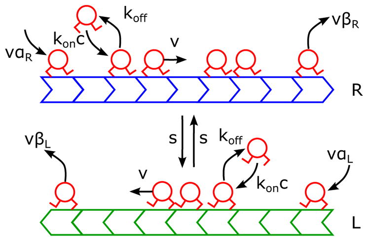
Schematic of the antiparallel two-lane TASEP with Langmuir kinetics and lane switching. Two lanes (green and blue) have their plus ends (indicating the direction of motor motion) oppositely oriented. The blue lane (R) has plus end to the right; the green lane (L) has plus end to the left. Motors (red) bind to empty lattice sites with rate konc, where c is the bulk motor concentration, and unbind with rate koff. Bound motors step toward the lane plus end with rate v (if the adjacent site toward the plus end is empty) or switch to the other lane with rate s (if the corresponding site on the adjacent lane is empty). At minus ends, motors are inserted at rate αR,Lv. At plus ends, motors are removed at rate βR,Lv.
The discrete model is based on the occupation number n̂i, which is 1 (0) if site i is occupied (empty). For bulk sites (2 < i < N − 1) on lanes with plus end right (R) and left (L), the equations are
| (1) |
| (2) |
where the angle brackets denote the sample averages. The boundary site equations include fluxes into and out of the lanes. The entering flux is vαR,L[1 − n̂1(t)], and the exiting flux is vβR,Ln̂N (t). We neglect binding and switching kinetics at the boundary sites. Then, we have
| (3) |
| (4) |
| (5) |
| (6) |
These boundary conditions fix the motor densities to be αR,L at the minus end and 1 − βR,L at the plus end of each lane.
We performed kinetic Monte Carlo (kMC) simulations of the discrete model with time step Δt. We applied the following rules for an overlap with N sites per lane.
Randomly choose a lane (R or L) and site i.
If the site is empty, attach a motor with probability koncΔt. If the site is occupied, detach the motor with probability koff Δt.
If the site is occupied and the adjacent site toward the plus end is empty, move the motor forward with probability vΔt.
If the site is occupied and the corresponding site on the neighboring lane is empty, switch the motor to the other lane with probability sΔt.
Enforce the boundary conditions: site 1 on lane R and site N on lane L are occupied with probability αR,L, while site N on lane R and site 1 on lane L are occupied with probability (1 − βR,L).
Repeat steps 1–5 2N times total to sample all sites on both lanes.
We chose Δt to give a characteristic time for motor binding and unbinding of about 105 time steps. For the reference parameter set and a bulk motor concentration of 200 nM, we used Δt = 5 × 10⁻⁴. Approximately 4 × 10⁷ time steps were used to reach steady state, then 2 × 10⁶ time steps were used to collect data. To determine the average motor concentration, we averaged 104 samples separated by 200 time steps. The reference parameter set was obtained from the BTS measurements [16] or estimated based on comparison of our kMC simulations to the BTS data [37] (Table I).
TABLE I.
Parameter values for the reference parameter set, taken from experimental measurements or estimated as noted.
| Symbol | Parameter | Reference value | Notes |
|---|---|---|---|
| v | Motor speed | 0.5 μm s−1 | Measured by Bieling et al. [16] |
| kon | Binding rate constant | 2.7 × 10⁻⁴nM−1 s−1 | Estimated based on motor density profiles and kymographs kymographs in Kuan and Betterton [37] |
| c | Bulk motor concentration | 1–200 nM | Varied by Bieling et al. [16] |
| koff | Unbinding rate | 0.169 s−1 | Measured by Bieling et al. [16] |
| s | Switching rate | 0.44 s−1 | Measured by Bieling et al. [16] |
| α | Motor flux constant into overlap from MT minus end | 0 | Motors bind primarily inside the overlap; see discussion in Kuan and Betterton [37]. We varied α between 0 and 1 to determine the model phase diagram |
| β | Motor flux constant out of overlap from MT plus end | 0 | An upper bound on the end motor unbinding rate is β = 2.7 × 10⁻³; see Kuan and Betterton [37]. We varied β between 0 and 1 to determine the model phase diagram |
| N | Number of sites | 1000 | We used N = 1000 unless otherwise specified |
A. Mean field continuum model
We derived the mean field continuum approximation to the model as in previous work [13,37]. We applied the stationary average 〈n̂i〉 ≡ ρi, the random phase approximation 〈n̂i n̂i+1〉 = 〈n̂i〉 〈n̂i+1〉, assumed motor commutation during switching 〈n̂R,i n̂L,i〉 = 〈n̂L,i〉 〈n̂R,i〉, and time derivative by taking Δt → 0. We then Taylor expanded to take the continuum limit and nondimensionalized by choosing the length of the overlap L as the unit of length and L/v as the unit of time. Capital letters denote the nondimensionalized parameters (S = sL/v, etc.). The position variable is changed from site index i to the position variable x, which ranges from −0.5 to 0.5. With x = 0 the center of the overlap, the boundary conditions become and . The steady-state continuum mean field equations are then
| (7) |
| (8) |
Because the equations are first-order differential equations, only one boundary condition is required for each. Since each end of the lane has two boundary conditions, the equations are overdetermined. The nonlinearities in these equations have a similar form to those of Burgers’ equation in fluid dynamics. Burgers’ equation also becomes overdetermined in the inviscid limit in which terms with second-order derivatives are neglected, which leads to the formation of shocks or domain walls which match solutions satisfying the two different boundary conditions [13,49,50]. Here, we denote xw the domain wall position where the solution that obeys the left boundary condition matches the solution that obeys the right boundary condition. The matching condition at the domain wall is continuity in the flux j(x) = ρ(x)[1 − ρ(x)], which can be written j(xw − ε) = j(xw + ε), where ε is infinitesimal. Since at the domain wall the density is not continuous, fulfilling the matching condition requires a density jump [13] of the form ρ(xw − ε) = 1 − ρ(xw + ε).
B. Total binding constraint
These equations satisfy a total binding constraint at steady state found by summing over all sites on both lanes [37]. In the discrete equations, the flux terms of the form n̂i−1(t)[1 − n̂i(t)] sum to zero and only the binding and boundary terms remain:
| (9) |
This gives a constraint on the summed motor occupancy
| (10) |
where we have defined the Langmuir density ρ0 = konc/(konc + koff). Therefore, at steady state an effective binding equilibrium that reflects binding, unbinding, and the lane-end boundary conditions must be reached on average for the entire system. This is related to the zero-current condition found in previous work on the two-lane antiparallel TASEP without binding kinetics [43,45].
In the continuum mean field model, the total binding constraint becomes
| (11) |
III. PHASE-PLANE SOLUTION
One solution to the steady-state mean field equations (7) and (8) is the constant solution at the Langmuir density ρ0 = Konc/(Konc + Koff). To study spatially varying solutions, we define the differences of the densities from . The equations can then be written
| (12) |
| (13) |
where we have defined the rate combinations k = Konc + Koff + S and γ = Konc − Koff, and Eqs. (12) and (13) are well defined for σR,L ≠ 0. We have not determined x-dependent expressions for σR (x) and σL(x) by solving these equations. Instead, we determined an implicit solution by first defining the sum and difference of the densities ϕ(x) = σR + σL and ω(x) = σR − σL. The equations become
| (14) |
| (15) |
which combine to give
| (16) |
Defining η(ϕ) = ω2(ϕ), this can be rewritten
| (17) |
or
| (18) |
This inexact ordinary differential equation (ODE) can be made exact through multiplication by the integrating factor (γ + 2Sϕ)k/S. We then obtain the solution by direct integration:
| (19) |
| (20) |
which gives the solution
| (21) |
Here, C1 and C denote integration constants. Equation (21) gives solutions for the density profiles in the ω-ϕ or σR-σL plane.
The integration constant C can be obtained by plugging in the boundary conditions , and . In much of this paper, we focus on the symmetric case for which αR = αL = α and βR = βL = β. Later in Sec. VI we discuss the general case when αR ≠ αL and βR ≠ βL.
A. Position-dependent approximate solutions
In Eqs. (12) and (13), position-dependent solutions can be derived by integrating
| (22) |
Since σL depends on x, this equation is difficult to integrate directly. However, since Eq. (21) gives the relationship between σR and σL, we can rewrite σL(x) = σL(σR). If we define , Eq. (22) can be written
| (23) |
This allows us to perform direct integration with an appropriate expansion of σL(YR).
B. Phase-space flow and fixed points
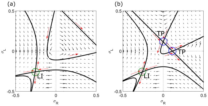
We can determine important features of the density profiles by studying Eqs. (12) and (13) in the σR-σL phase plane and determining the phase-space flows. In the phase plane, Eqs. (12) and (13) define an effective velocity field that shows the local change in σR and σL at each point in the plane (Fig. 2). Note that because the equations are unchanged under the operation R → L, x → −x, the phase field is symmetric under reflection about the line σL = σR.
FIG. 2.
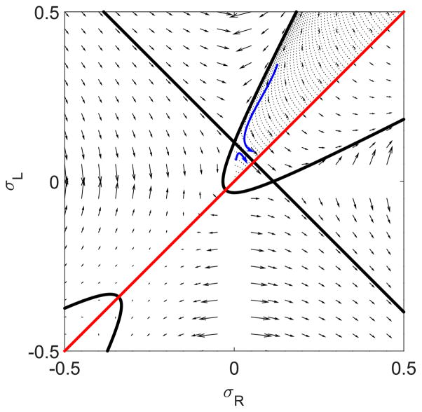
Flows in the σR-σL phase plane for low [(a), 0.1 s−1] and high [(b), 0.5 s−1] switching rates. Solid lines are trajectories that pass through the fixed points, as discussed in the text. The Langmuir isotherm is labeled LI and the transition points TP. The bulk motor concentration is 200 nM, the motor speed is 5 μm s−1, and other parameters are the reference values of Table I. Arrows indicate the vector field, which has the mathematical form of Eqs. (12) and (13).
The flow trajectories are controlled by the fixed points in the phase plane. There can be as many as three fixed points: the Langmuir isotherm (LI), and two transition points (TP) that appear for sufficiently high switching rate. Figure 2 shows the fixed points for low switching rate (left) and high switching rate (right). To determine the fixed points, we rearrange Eq. (21) to solve for the integration constant:
| (24) |
The transition line and points can be determined by the trajectories with C = 0. In this case, either the first term (γ + 2Sϕ)1+k/S or the second term in square brackets is zero. If the first term is zero, then γ + 2S(σR + σL) = 0. This is a line with slope −1 in the σR-σL plane that intercepts σL = 0 at the point σR = (Koff − Konc)/(2S). This line can also be derived by setting Eq. (14) to zero. This is equivalent to requiring that the total density ϕ = σR + σL be independent of x; in this case ω(γ + 2Sϕ)]/(ϕ2 − ω2) = 0, leading to γ + 2S(σR + σL) = 0 as above. Physically, this means that the switching and binding terms balance. This line is called the transition line, and the transition points occur where this line crosses the σR = 0 and σL = 0 lines. Since the flow values are ill defined at the transition points (one of dσR,L/dx is ill defined), they can only lie on σR,L = 0 lines.
If the second term in square brackets is zero, the solution is a hyperbola that satisfies
| (25) |
The line and hyperbola solutions are shown in Figs. 2 and 3. The hyperbola intersects the transition line at the transition points.
FIG. 3.
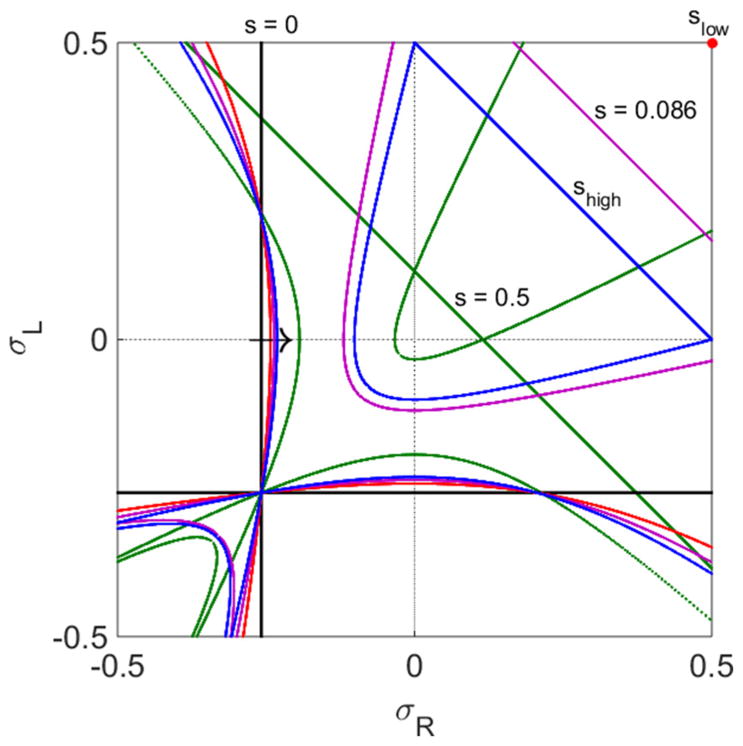
Changes in trajectories and fixed points with varying switching rate. Curves with s = 0 s−1, black; , purple; s = shigh ≈ 0.1150 s−1, blue; s = 0.5 s−1, green. The red point labels slow. The arrow indicates how the curve with CLI changes as s increases. The bulk motor concentration is c = 200 nM and motor speed is 5 μm s−1; other parameters are the reference values of Table I.
The position of the transition line and points allows us to define two critical switching rates. When S increases to the value Slow = (Koff − Konc)/2, the transition line first intersects . This allows the Hn phase to appear for Slow < S < Shigh (as discussed in Sec. V). When S > Shigh = Koff − Konc, the transition points appear. This upper critical switching rate occurs when the transition line first intersects and (0, ). This allows appearance pof the LHLH phase (as discussed in Sec. V).
The general case in Eq. (24) can be understood as an exponential-like term [because the term (γ + 2Sϕ)1+k/S reduces to an exponential if S → 0] times a hyperbola term. The hyperbola has foci and, in general, two intersections on the σR = σL line. Multiplying by the exponential term does not change these properties qualitatively, if it remains real. For the special value
| (26) |
the two intersections of the curves with the σR = σL line become one intersection [51]. The intersection is the LI. At the Langmuir isotherm, the density on each lane is the Langmuir density set by binding or unbinding equilibrium. As a result, . We note that in the limit S → 0, these curves merge with the C = 0 curves discussed above. In this limit, CLI = 0.
1. Domain walls
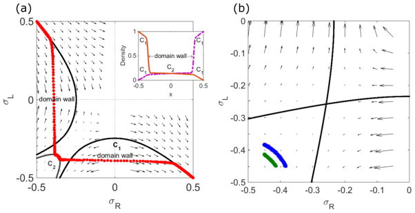
In principle, the phase-plane density profile can be determined by following the local velocity field, connecting the two points on the plane that correspond to the lane end boundary conditions. Indeed, if the boundary points both lie in the same quadrant of the plane, the solution follows the local flow. However, in many cases the boundary points lie in different quadrants, so that the boundary points cannot be connected without crossing the lines σR = 0 or σL = 0 where Eqs. (12) or (13) are ill defined. Then, the solution will contain a domain wall at position xw that must satisfy the matching condition σ(xw − ε) = −σ(xw + ε) (as discussed in Sec. II A). In the phase plane, a domain wall therefore appears as sign change of one of the densities (Fig. 4).
FIG. 4.
Effects of domain walls and finite size on density profiles. Left, determination of domain wall positions in the phase-plane trajectory and the density profile (inset). Red points show kMC simulation results. The boundary points are and . The solution locally follows the flow, which cannot connect the boundary points without crossing the lines with σR = 0 and σL = 0 where the velocity is ill defined. Crossing these lines uses the matching condition to connect to another exact solution curve, introducing a domain wall. Inset shows the density profiles of ρR (purple, dashed) and ρL (brown, solid). The sharp transitions in ρR and ρL indicate the domain walls. There are three regions which are separated by two domain walls: regions near ends follow C1, and the region at the center is described by C2. Right, finite-size constraint. The blue points (longer curve) are kMC simulation results for N = 1000, and the green (shorter curve) N = 500. For a larger number of sites, the dimensionless motor speed is smaller, moving the solution closer to the LI. The switching rate is 0.44 s−1(left), 0.1 s−1(right), the bulk motor concentration c = 200 nM, and the motor speed 5 μm s−1; other parameters are the reference values of Table I. Arrows indicate the vector field, which has the mathematical form of Eqs. (12) and (13).
2. Finite-size constraint
The solutions are also affected by the finite-size constraint. If, for example, each lane has 1000 sites, the correct trajectory should connect the boundary points with exactly 1000 sites. The number of sites controls the effective magnitude of dx, and is therefore analogous to time in the flow. Thus, the faster the effective flow, the smaller the number of sites traversed in position space. At the Langmuir isotherm, the number of sites can be infinite since this point has zero flow velocity [52]. As the total number of sites increases, the trajectory will approach closer to the LI because this point is the only one which can contain an infinite number of sites (Fig. 4). The finite-size constraint can prevent the solution from exactly following the phase-space flow. As a result, the boundary conditions are not always satisfied. This is discussed further in Sec. IV.
IV. NONEQUILIBRIUM PHASES FOR SYMMETRIC BOUNDARY CONDITIONS
The nonequilibrium steady-state solution of TASEP models sensitively depends on the boundary conditions α and 1 − β [4]. Because the flux ρ(1 − ρ) is maximized for an occupancy of , the phase with bulk density of is called the maximum-current phase. The high-density phase has bulk density and the low-density phase has bulk density . In the single-lane TASEP with LK, PFF found a low-density–high-density coexistence phase and a Meissner phase, but no maximum current phase [13].
In our antiparallel two-lane model with binding and switching kinetics, we find the same phases that appear in the single-lane case. In addition, we find a four-phase coexistence low-density–high-density–low-density–high-density (LHLH) phase, as discussed below. In addition, the nonzero switching rate in our model that couples the two lanes means that the central density is not only attracted to the Langmuir isotherm and repelled from the maximum current lines, but also attracted by the transition line. This competition can cause either a local maximum or minimum of the density at the overlap center (x = 0). If the total density ρR (x) + ρL(x) has a local maximum (minimum) at x = 0, we denote it a local maximum (minimum) phase. The occurrence of local maxima (minima) also occurs in the single-lane case [13], although PFF did not treat it as separate feature of the phase since it has a less pronounced effect there than in the antiparallel lane case where the overall density is the sum of the two single-lane densities.
Here, we focus on the case of symmetric boundary conditions with αR = αL = α and βR = βL = β. We first discuss the stability of the boundary conditions and properties of the central density. Then, we describe each phase and how we determine the phase boundaries. We focus on the case . Because the system has particle-hole symmetry, the case can be understood by the transformation ρ → 1 → ρ.
A. Domain wall motion
In the steady-state TASEP, the boundary conditions are not always satisfied at the boundary sites (or continuously approaching the boundary). The stability of the boundary density values was determined for the single-lane TASEP by Kolomeisky et al. [10], who worked out the speed at which a domain wall moves. When α and , the domain wall velocity is , where jr,l denotes the current at the right and left boundaries. If we take ρl = α, jl = α(1 − α), ρr = β, and jr = β(1 − β), the domain wall velocity is β − α. Therefore, if β > α the domain wall moves to the right end of the system and the right boundary condition is not satisfied, while if β < α the left boundary condition is not satisfied.
A similar relation can be determined for matching a high-density region to a maximum-current region with a domain wall [10]. Suppose and , but a maximum-current phase appears on the left so that jl becomes . The domain wall velocity becomes , which gives an unstable left boundary condition. Similar behavior occurs if and .
These relations no longer strictly hold when binding kinetics or switching between multiple lanes are added to the model. However, they are a valuable starting point to gain intuition about the stability of domain walls due to the TASEP.
B. Properties of the central density
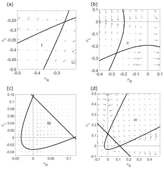
When the boundary conditions are symmetric, the total density is symmetric about x = 0. Therefore, ρR (0) = ρL(0) and the density in the center of the system must lie on the σR = σL line. The σR = σL line can be separated into four regions, which correspond to four different possible behaviors of the central density (Figs. 2 and 5).
FIG. 5.
Illustration of the four regions of the central density, as defined in the text. The switching rate is 0.5 s−1, the bulk motor concentration c = 200 nM, and the motor speed is 5 μm s−1; other parameters are the reference values of Table I. Arrows indicate the vector field, which has the mathematical form of Eqs. (12) and (13).
Region I occurs where σR = σL and the density is less than the Langmuir isotherm. In this region, the flow makes the density approach the LI. At the isotherm, the rates of change of both σR and σL are zero, and as the flow approaches the LI, these rates of change decrease. Therefore, the density remains less than or equal to the Langmuir isotherm. This makes the central density a local maximum, which we denote a local maximum phase. Region II occurs where σR = σL and the density is greater than the Langmuir isotherm, but less than 0. In this region, the flow makes the density approach the LI, decreasing the density. The density remains greater than or equal to the Langmuir isotherm. This makes the central density a local minimum, which we denote a local minimum phase.
Regions III and IV occur where σR = σL and the density is greater than 0 but less than (region III) or greater than (region IV) the transition line. The transition line occurs where the effects of switching and binding kinetics balance. In region III, binding kinetics are more important, while in region IV, switching kinetics are more important. In both of these regions, the central density is on a single lane. Because the density is greater than the LI, the mean field binding and unbinding terms in Eqs. (7) and (8) are net negative. As a result, the flux term becomes negative. Therefore, the flux decreases as the density increases. Another way to see this is to note that the flux has a maximum for 0 ≤ ρ ≤ 1 when . For , the flux increases as density increases, while if , the flux decreases as density increases. The net effect is to cause the density to increase approaching the σR = σL line in region III. Therefore, the central density has a local maximum in region III. However, in region IV, σR and σL are larger, causing the switching terms to contribute significantly to the flow. This gives a positive contribution in Eqs. (7) and (8). Therefore, the flow changes the sign in region IV (compared with region III). The central density has a local minimum in region IV.
C. Nonequilibrium phases
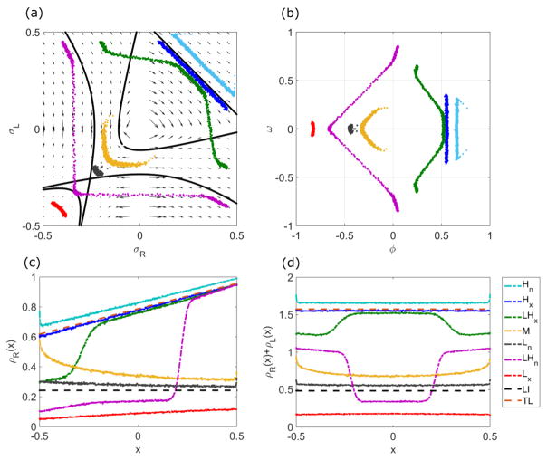
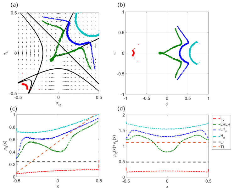
Here, we discuss the nonequilibrium phases that occur in our model, as illustrated in Figs. 6 and 7. There are five possible phases: low density, high density, low density–high density, low density–high density–low density–high density, and Meissner. As mentioned above, we focus on the case with .
FIG. 6.
Examples of the nonlinear phases for low switching rate. (a) Trajectories in the σR-σL plane. (b) Trajectories in the ϕ-ω plane, where ϕ = σR + σL and ω = σR − σL, illustrating the local maxima and minima of the central density. (c) The density in lane R, ρR (x). The black dashed line (flat) indicates the LI in position space, and the brown dashed line (tilted) is the transition line in position space. (d) The total density as a function of position. The black dashed line indicates the LI (its value is 2ρ0 since it is ρR + ρL) in position space, and the brown dashed line is the transition line in position space (its value is since it is ρR + ρL). The boundary conditions are (α,1 − β) = (0.05,0.1) (red), (0.1,0.95) (purple), (0.3,0.4) (gray), (0.6,0.4) (yellow), (0.3,0.95) (green), (0.6,0.95) (blue), and (0.95,0.99) (cyan). The switching rate is 0.1 s−1, the bulk motor concentration c = 200 nM, and the motor speed 5 μm s−1; other parameters are the reference values of Table I. Arrows in (a) indicate the vector field, which has the mathematical form of Eqs. (12) and (13).
FIG. 7.
Examples of the nonlinear phases for high switching rate. (a) Trajectories in the σR-σL plane. (b) Trajectories in the ϕ-ω plane, where ϕ = σR + σL and ω = σR − σL, illustrating the local maxima and minima of the central density. (c) The density in lane R, ρR (x). The black dashed line (flat) indicates the LI in position space, and the brown dashed line (tilted) is the transition line in position space. (d) The total density as a function of position. The black dashed line indicates the LI (its value is 2ρ0 since it is ρR + ρL) in position space, and the brown dashed line is the transition line in position space (its value is since it is ρR + ρL). The boundary conditions are (α, 1 − β) = (0.05,0.6) (red), (0.3,0.9) (green), (0.3,0.95) (blue), and (0.9,1.0) (cyan). The switching rate is 0.5 s−1, the bulk motor concentration c = 200 nM, and the motor speed 5 μm s−1; other parameters are the reference values of Table I. Arrows in (a) indicate the vector field, which has the mathematical form of Eqs. (12) and (13).
Low density (L)
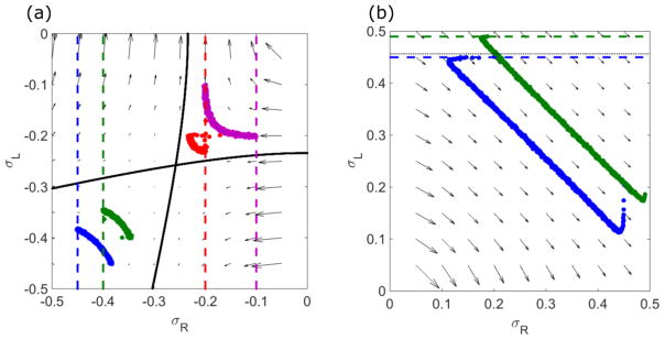
The density in each lane remains . The L phase occurs when and the right boundary condition cannot be satisfied. According to the behavior of the local maxima and minima derived above in Sec. IV B above, if α < LI, the central density is a local maximum; if α > LI, the central density is a local minimum (Fig. 8 right).
FIG. 8.
Example phase-plane trajectories of L and H phases. (a) L phase. The starting and ending points are (σR, σL) = (−0.45, −0.4) and (−0.4, −0.45) (blue), (−0.4, −0.45) and (−0.45, −0.4) (green), (−0.2, −0.1) and (−0.1, −0.2) (red), and (−0.1, −0.2) and (−0.2, −0.1) (purple). The dashed lines show that the L phase obeys the left boundary conditions, where the positions are σR = −0.45 (blue), σR = −0.4 (green), σR = −0.2 (red), and σR = −0.1 (purple). (b) H phase. The starting and ending points are (σR, σL) = (0.3, 0.45) and (0.45, 0.3) (blue), (0.2, 0.49) and (0.49, 0.2) (green). The dashed lines show that the H phase obeys the right boundary conditions, where the positions are σL = 0.45 (blue) and σL = 0.49 (green). The black dashed line , the critical density ρc (see text) of the local minimum and local maximum phases. The switching rate is 0.1 s−1, bulk motor concentration c = 200 nM, and motor speed 5 μm s−1; other parameters are the reference values of Table I. Arrows indicate the vector field, which has the mathematical form of Eqs. (12) and (13).
High density (H)
The density in each lane remains . The H phase occurs when and so that the left boundary condition cannot be satisfied. There is a critical concentration we denote ρc which corresponds to the density where the transition line crosses the σR = σL line. If 1 − β < ρc, the central density is a local maximum, while if 1 − β > ρc, the central density is a local minimum (Fig. 8 left).
Low-density–high-density coexistence (LH)
In this phase, the steady-state density on each lane has both low-density and high-density regions. A domain wall occurs where the low- and high-density phases meet; we call the length of the high-density region the boundary-layer length [37]. We discuss how the domain wall position is determined in more detail in Sec. V. The boundary-layer length determines whether the overlap shows greater motor accumulation at the center or at the ends: if the boundary-layer length is greater than half the overlap length, the overall density is higher at the overlap center (since we set our ). We note that this condition is distinct from whether or not a local maximum or minimum occurs at the overlap centers, as discussed above. The local extremum is identified using the derivative d(σR + σL)/dx at the overlap center.
Low density–high density–low density–high density (LHLH)
For sufficiently high switching rate, a multiphase coexistence region can appear in the LH region (Fig. 7). To understand why the LHLH phase occurs, note that the transition line (Fig. 2 left) divides the phase plane into two regions. If a boundary point is above the transition line in the upper left quadrant, the flow does not reach the σL = 0 line, where a jump into region II is possible (Fig. 5) in order to connect the flow to the other boundary condition [53]. Thus, the only allowed domain wall involves a jump to the upper right quadrant (outside of the hyperbola), followed by further motion along the flow field. The solution then jumps to region II because the flow outside the hyperbola will not cross the line σR = σL. These multiple jumps cause multiple domain walls to appear. We note that the LHLH phase is reminiscent of LD-BP-HD multiphase coexistence found by Pierobon et al. [47], which arises from a point defect on a single lane.
Meissner (M)
In the pure TASEP, the maximum current phase occurs when the bulk density profile is independent of the boundary conditions [4]. The analogous phase in the TASEP with LK is the Meissner phase [13]. Neither of the boundary conditions is satisfied in this phase.
V. PHASE DIAGRAM FOR SYMMETRIC BOUNDARY CONDITIONS
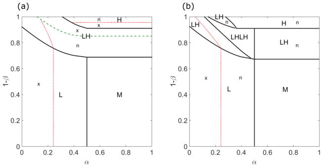
Figure 9 shows typical phase diagrams illustrating the regions where the five phases (L, H, M, LH, and LHLH) appear as a function of the boundary conditions α and 1 − β. These boundary motor densities define the boundary points in the phase plane (Fig. 2). To determine the phase diagram, it is convenient to determine trajectories on the phase plane. The phase regions are the collection of all the boundary points which show the same physical behavior (Figs. 6 and 7). As noted above, we study . The phase boundaries are determined as follows:
FIG. 9.
The phase diagrams for low [(a), 0.1 s−1] and high [(b), 0.5 s−1] switching rates. The phases are L (low density), M (Meissner), H (high density), LH (low-density–high-density coexistence), and LHLH (low-density–high-density–low-density–high-density coexistence). The thick green dashed line indicates where the domain wall position xw = 0, which separates regions with a local maximum of the central density (x) or local minimum (n). The red dashed lines indicate boundaries between local maximum and minimum phases. For low switching rate, the left parts of the L and LH phases are local maximum phases, and the right are local minimum phases. The upper part in the H phase is local minimum phase. For high switching rate, the left parts of the L and LH phases are local maximum phases, and the right parts are local minimum phases. The bulk motor concentration is c = 200 nM, and the motor speed 5 μm s−1; other parameters are the reference values of Table I.
Boundary between L and M phases
The phase boundary between L and M occurs where because the boundary conditions cannot be satisfied when and . The phase in which none of the boundary conditions are satisfied defines the Meissner phase [13].
Boundaries of the LH phase
The low-density–high-density coexistence phase contains a domain wall, at which the density changes discontinuously but the flux ρ(1 − ρ) remains continuous [13]. Across the domain wall, the matching condition σ(xw − ε) = −σ(xw + ε) must be satisfied. The boundaries of the LH phase occur when the domain wall position xw moves outside the lane, that is, when .
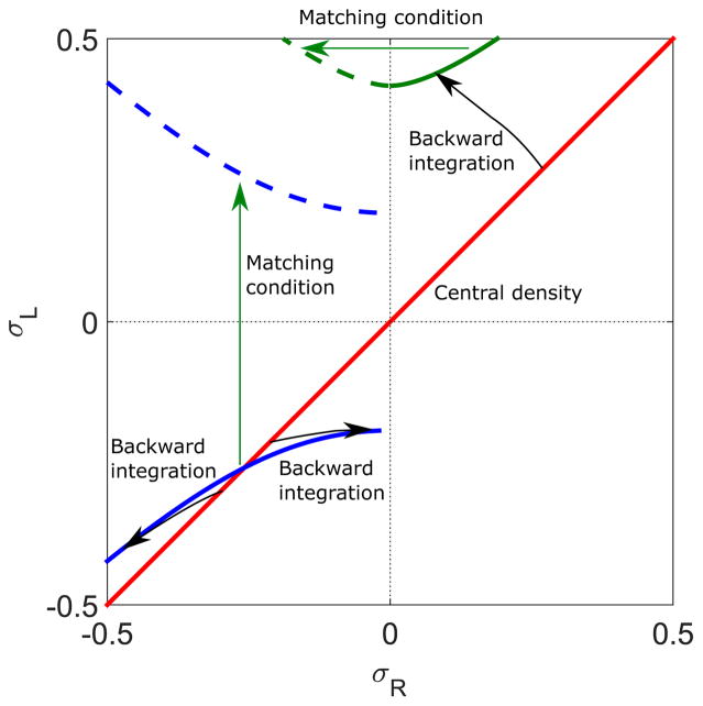
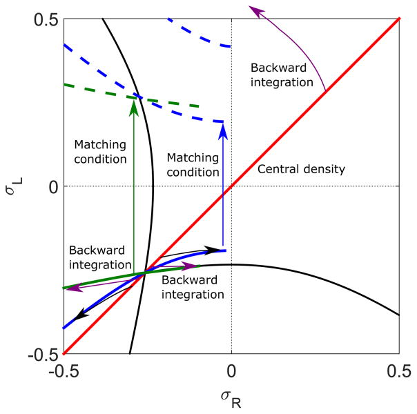
To determine the domain wall position, we integrate the density profile back from the center (x = 0) to , thereby determining . Because the system is symmetric, the central density σR,L(x = 0) must lie on the line σR = σL (Fig. 2). By integrating the density to , we can map the line of slope 1 to the set of points (Fig. 10, black arrows to blue solid lines). If we apply the matching condition to this set of points to jump them to positive values of σL, we have found the set of points for which the domain wall occurs at . This is equivalent to an L phase that extends to the right end of the lane (Fig. 10, green arrow to blue dashed lines). This defines the phase boundary of the LH phase (Fig. 10, blue dashed line). Using the same analysis, we draw another phase boundary of the LH phase when the domain wall position is at , which is equivalent to the boundary for which the high-density phase extends to the left end of the system (Fig. 10, green dashed line).
FIG. 10.
Illustration of calculation of the LH phase boundary. The red line indicates the central density, which lies on the σR = σL line for symmetric boundary conditions. Backward integration from this line (black arrows) to gives the thick blue and green, where the blue line corresponds to σ < 0 and green line σ > 0. Applying the matching condition to σL and σR (green arrows) gives the dashed blue and green lines, respectively. These are the phase boundaries of the LH phase. The switching rate is 0.1 s−1, bulk motor concentration c = 200 nM, and motor speed 5 μm s−1; other parameters are the reference values of Table I.
In the upper right quadrant of the phase plane (σR,L > 0), the left boundary condition cannot be satisfied, so the LH phase boundaries are the horizontal lines which define the upper boundary of the M phase. If the domain wall position is greater than , the right boundary condition is no longer satisfied, and vice versa for case. Thus, the region under the lower boundary of the LH phase and does not satisfy the right boundary condition. In addition, means that the left boundary condition is not satisfied. Therefore, this region is the Meissner phase.
Since the phase boundaries depend on assuming that the points σR,L(x = 0) lie on the σR = σL line, the width of the phases and the shape of the phase boundaries depend on the number of sites in the lanes and the motor speed. The faster the speed or the lower the number of sites, the smaller the dimensionless values of Konc, Koff, and S. This leads to a smaller magnitude of the phase-plane flow velocity. Since the integration of the densities from x = 0 to is inversely proportional to the flow velocity , decreases in motor speed make the phase boundary lines closer to the line σR = σL. However, the line dividing the L and LH phases always passes through the Langmuir isotherm since the phase-space flow velocity is zero at the Langmuir isotherm. Similarly, slower motor speed or higher number of sites in the overlap makes the set of points obtained by integrating backward move closer to the trajectory line that passes through the Langmuir isotherm (Fig. 11).
FIG. 11.
Illustration of the effects of changing motor speed on the LH phase boundary. High motor speed (5 μm s−1) shown in blue, low motor speed 0.5 μm s−1 shown in green. The red line indicates the central density, which lies on the σR = σL line for symmetric boundary conditions. Backward integration from this line (black and purple arrows) to gives the thick blue and green lines. Applying the matching condition to σL and σR (blue and green arrows) gives the dashed blue and green lines. These are the phase boundaries of the LH phase. The solid black lines are trajectories which pass through the Langmuir isotherm. For lower motor speed, backward-integrated line moves closer to the black line. The phase boundary of the LH and H phases is outside of the lanes. The switching rate is 0.1 s−1, the bulk motor concentration c = 200 nM; other parameters are the reference values of Table I.
Once the domain wall position decreases to xw < 0, the longer length of the high-density region makes the overall central density greater than the end density. This determines whether the center of the lanes has a local maximum or local minimum; these two cases are distinguished by the thick dashed line in the phase diagram (Fig. 9, left). If xw = 0, then the central density must lie on the line σR = −σL because then by the matching condition the density can jump to the line σR = σL and then jump to σR = −σL. Therefore, the set of starting points that correspond to domain wall positions with xw = 0 is calculated by integrating backwards from the σR = −σL line to determine .
The weak dashed line in the LH phase indicates whether a local maximum or minimum occurs (Fig. 9). If the domain wall is in region I, the central density is a local maximum, while if domain wall is in region II, the central density is a local minimum. By integrating backwards from (the point at which the domain wall position overlaps with the Langmuir isotherm), we can determine the dividing line between the local maximum and minimum regions [54].
Boundaries of the LHLH phase
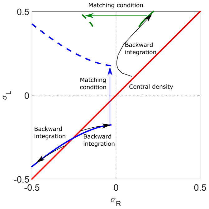
When we integrate backwards from the σR = σL line, it is not possible to reach the σR = 0 line if the switching rate is high (Fig. 12). The transition line then separates the set of backwards integrated points into two regions (regions III and IV described in Sec. IV B, Fig. 13). The LHLH phase appears in the region between σR = 0 and the LH phase boundary.
FIG. 12.
Illustration of calculation of the LHLH phase boundary. The red line indicates the central density, which lies on the σR = σL line for symmetric boundary conditions. The thick black lines are the line and hyperbola determined from Eq. (21) with C = 0. The dashed black lines are trajectories determined by backward integration from σR = σL line. The blue curves show the flow directions. The switching rate is 0.5 s−1, bulk motor concentration c = 200 nM, and motor speed 5 μm s−1; other parameters are the reference values of Table I. Arrows indicate the vector field, which has the mathematical form of Eqs. (12) and (13).
FIG. 13.
Illustration of calculation of phase boundaries. The red line indicates the central density, which lies on the σR = σL line for symmetric boundary conditions. Backward integration from this line (black arrows) to gives the thick blue and green lines, where the blue line corresponds to σ < 0 and green line σ > 0. Applying the matching condition to σL and σR (blue and green arrows) gives the dashed blue and green lines, respectively. These are the phase boundaries of the LH phase. The green dashed line stops around σR = −0.1386 and will not extend to σR = 0 line. The switching rate is 0.5 s−1, bulk motor concentration c = 200 nM, and the motor speed 5 μm s−1; other parameters are the reference values of Table I.
Boundaries of the H phase
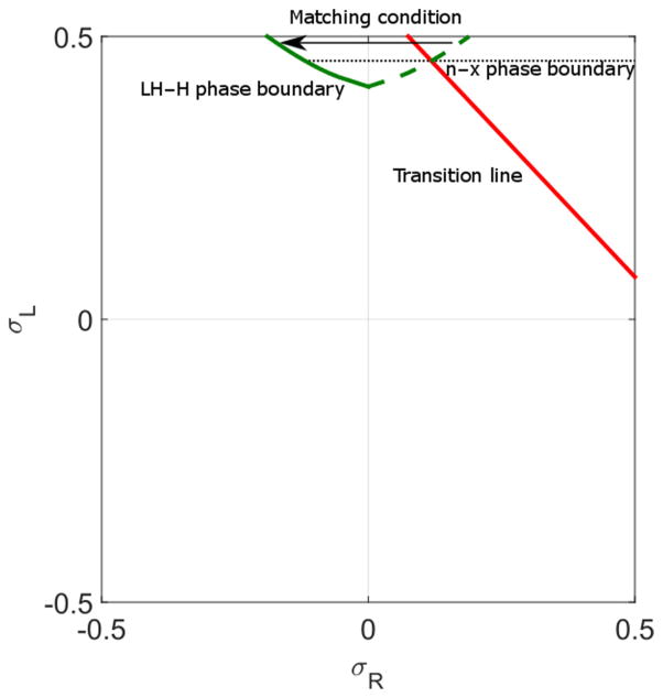
The region in the phase diagram with high values of 1 − β (small β) above the LH phase corresponds to the high-density phase. In the H phase, the lane left-end boundary condition is not satisfied. This phase is divided into two regions in which the central density has a local maximum or local minimum, controlled by the transition line. We determine the separation between these two behaviors by determining where the set of points (integrated backwards from the σR = σL line) intercept the transition line (Fig. 14).
FIG. 14.
Illustration of calculation of phase boundaries of local maximum and minimum phases. The dashed green line is obtained from backward integration of the σR = σL line to . The green line indicates the LH phase boundary determined by the matching condition, where the right of the line is the H phase. The red line is the transition line. Since the H phase satisfies the right boundary condition, the starting point of the density profile depends on σL value. Therefore, the phase boundary of the local maximum and minimum phase is a horizontal line that intersects the green dashed line and the transition line. The local minimum phase is above the black dashed line. The switching rate is 0.1 s−1, bulk motor concentration c = 200 nM, and motor speed is 5 μm s−1; other parameters are the reference values of Table I.
A. Approximate phase boundaries using the total binding constraint
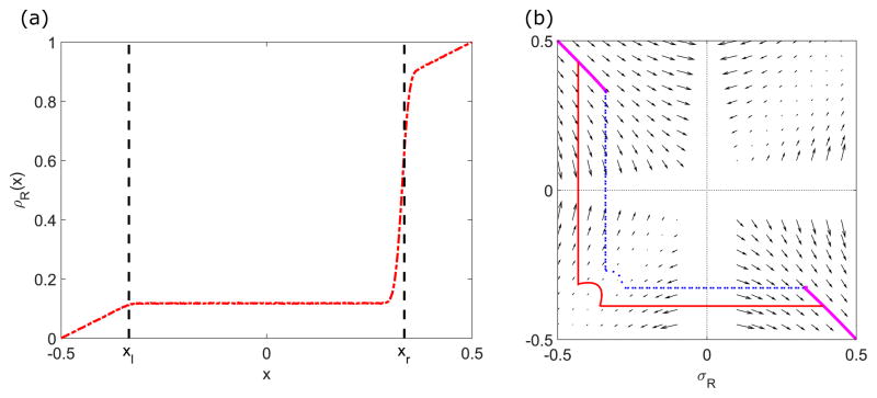
Phases that include domain walls mean that the density profile does not always exactly satisfy the first-order mean field steady-state equations (7), (8), and (21). The density is separated into several regions (Fig. 15). In principle, there could be multiple possible trajectories which satisfy the boundary conditions and locally satisfy the differential equations (Fig. 15, right). Despite the possibility of multiple solutions for the same boundary conditions, our kMC simulation results typically find just one stable steady-state solution for each set of boundary conditions.
FIG. 15.
Illustration of the density profile (a) and hypothetical phase-plane trajectories (b) in the LH phase. (b) The thick purple curves indicate the density profile starting from the boundary conditions, and the dashed blue and solid red curves are two different hypothetical trajectories which locally obey Eqs. (7), (8), and (21). The parameters are s = 0.44 s−1, c = 200 nM, v = 5 μm s−1, kon = 2.7 × 10⁻⁶ nM−1 s−1, and koff = 0.00169 s−1; other parameters are the reference values of Table I. Arrows in (b) indicate the vector field, which has the mathematical form of Eqs. (12) and (13).
To understand this, we consider the number of equations and unknowns. We focus on a single lane, e.g., the R lane. From Eq. (23), we can derive the density profile starting from the left end and the left boundary condition αR. We integrate to the domain wall position xl; the corresponding density profile is ρ(xl). We have two unknowns [xl and ρ(xl)] and one equation (23). Using the same argument beginning from the right end of the lane, we have two unknowns [xr and ρ(xr)] and one equation (23). Then, we can determine the density profile between xl and xr using Eq. (21) or (23) with boundary conditions ρ(xl) and 1 − ρ(xr) [55]. This adds no new variables and one equation (23). Thus, there are four unknown variables: xr, xl, ρ(xr), and ρ(xl), and three equations. We need one more equation in order to uniquely determine the density profile. As discussed above in Sec. III B, this can be done numerically using the finite-size constraint. Alternatively, we can use the total binding constraint of Eq. (11), as discussed in our previous work [37]. Satisfying one of these constraints automatically satisfies the other. The total binding constraint is useful because it can be combined with analytic approximations to the position-dependent density profile [Eq. (23)].
Here, we illustrate how to use the total binding constraint to derive analytic estimates for the LH phase boundaries. For symmetric boundary conditions, the domain wall positions are also symmetric, so xr = −xbl and xl = xbl. If we consider the limit of large motor speed, Eqs. (12) and (13) can be approximated by a piecewise linear form [37]
| (27) |
Using the total binding constraint of Eq. (11), the integral of the density is
| (28) |
The phase boundary between the LH and L phases occurs when the domain wall position is . Then, Eq. (28) simplifies to
| (29) |
or
| (30) |
Similarly, the phase boundary between the LH and H phases is found by considering a piecewise-linear density profile like that above, but with a jump to high density at xl. In this case, the approximate density profile is
| (31) |
As above, the phase boundary between the LH and H phases occurs when the domain wall position is (note that xbl is positive in our convention), giving a relation from the total binding constraint of
| (32) |
or
| (33) |
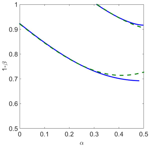
Figure 16 shows the result of determining the LH phase boundaries using this approximation and the total binding constraint. It agrees well with the numerically determined boundaries, particularly for small α.
FIG. 16.
Comparison of determination of the L phase boundaries using the total binding constraint with linear approximation [green dashed curves, Eqs. (27) and (31)] and the finite-size constraint without any approximation (blue solid curves). The switching rate is 0.1 s−1, bulk motor concentration c = 200 nM, and motor speed 5 μm s−1; other parameters are the reference values of Table I.
VI. NONEQUILIBRIUM PHASES FOR GENERAL BOUNDARY CONDITIONS
In general, the boundary conditions might not be symmetric for the two lanes: αR ≠ αL and βR ≠ βL. In this case, we cannot determine the density profile using the symmetry argument that the central density lies on the σR = σL line. However, we can still use the properties of the analytic solution to the mean field steady-state equations and the phase-space flow to determine properties of the solutions. The density profile locally follows the phase-space flow, and is connected by a curve with the correct number of sites that links the left boundary condition to the right boundary condition . The matching condition for the domain wall can be applied, if necessary. We can describe the possible behaviors based on whether or not each of the four boundary conditions if satisfied. This gives 24 = 16 possible cases, which can be grouped into 10 classes illustrated in Figs. 17 and 18.
FIG. 17.
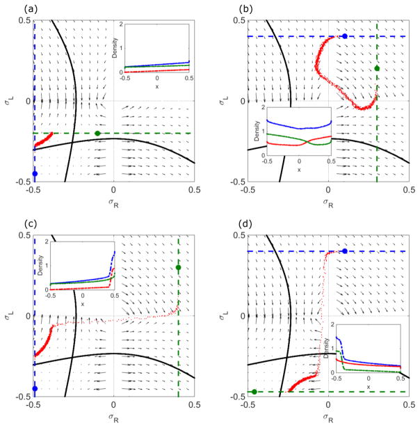
Example phase-plane trajectories and density profiles (inset) for general boundary conditions. Insets show ρR + ρL (blue), ρR (red), and ρL (green). Red dots are kMC simulation results. The blue dot indicates the left boundary condition and the green dot the right boundary condition. (a) The blue line is , and the green line is . (b) The blue line is , and the green line is . (c) The blue line is , and the green line is . (d) The blue line is , and the green line is . The switching rate is 0.1 s−1, bulk motor concentration c = 200 nM, and motor speed 5 μm s−1; other parameters are the reference values of Table I. Arrows indicate the vector field, which has the mathematical form of Eqs. (12) and (13).
FIG. 18.
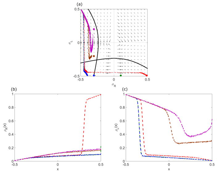
Example phase-plane trajectories and density profiles for general boundary conditions, illustrating how altering the right boundary condition changes the density profile. (a) Colored dots indicate the right boundary condition. Red curve satisfies all four boundary conditions; green, blue, and brown curves do not satisfy βR ; and the purple curve satisfies αR and βL. (b), (c) Corresponding density profiles on the R lane (b) and L lane (c). The switching rate is 0.1 s−1, bulk motor concentration c = 200 nM, and motor speed 5 μm s−1; other parameters are the reference values of Table I. Arrows in (a) indicate vector field, which has the mathematical form in (12) and (13).
The location of the boundary conditions in the phase plane determines the types of behavior that can occur. We will therefore consider which quadrant in the phase plane (upper right, upper left, lower left, lower right) contains the left ( ) and right ( ) boundary conditions.
All boundary conditions satisfied
This case is analogous to the LH phase in the symmetric phase diagram. It often occurs when the left boundary condition ( ) is in the upper left quadrant of the phase plane and the right boundary condition ( ) is in the lower right quadrant. A domain wall occurs either in the upper right or lower left quadrant.
No boundary conditions satisfied
This case is analogous to the M phase in the symmetric phase diagram. It often occurs when the left boundary condition is in the lower right quadrant and the right boundary condition is in the upper left quadrant. The density profile is independent of the boundary conditions.
Both lane minus-end boundary conditions satisfied
This case is analogous to the L phase in the symmetric phase diagram. It often occurs when the left boundary condition and the right boundary condition are in the lower left quadrant. The density profile follows a trajectory which obeys , and contains the correct number of sites [Fig. 17(a)].
Both lane plus-end boundary conditions satisfied
This case is analogous to the H phase in the symmetric phase diagram. It often occurs when the left boundary condition and the right boundary condition are in the upper right quadrant. The density profile follows a trajectory which obeys , and contains the correct number of sites [Fig. 17(b)].
Both lane minus-end and one plus-end boundary conditions satisfied
This case is analogous to a semi-LH phase. It can occur two ways, depending on whether lane L or R has its plus-end boundary condition satisfied. The L case often occurs when the left boundary condition is in the upper left quadrant and the right boundary condition is in the lower left quadrant. This phase occurs when the right boundary point moves from the lower right quadrant (where all boundary conditions can be satisfied) to the lower left quadrant. The domain wall of the R lane moves beyond , so that the right boundary condition for the R lane is not satisfied.
The R case is symmetric with the L case. It occurs when the left boundary condition is in the lower left quadrant and the right boundary condition is in the lower right quadrant. This phase occurs when the left boundary point moves from the the upper left quadrant (where all boundary conditions can be satisfied) to the lower left quadrant. The domain wall of the L lane moves beyond , so that the left boundary condition for the L lane is not satisfied.
Left or right boundary conditions satisfied
This case is analogous to a semi-LH phase. First, we consider when the left boundary condition is satisfied. This often occurs when both the left and right boundary conditions are in the upper left quadrant. This case can be treated as moving the right boundary condition from the lower left quadrant to the upper left quadrant. Once the right boundary condition passes the σL = 0 line, the flow cannot reach the right boundary condition, even with a domain wall. Therefore, the density profile is dominated by the left boundary condition only.
The case in which the right boundary condition is satisfied is symmetric. This often occurs when both boundary conditions are in the lower right quadrant. This case can be treated as moving the left boundary condition from the lower left quadrant to the lower right quadrant. Once the right boundary condition passes the σR = 0 line, the flow cannot reach the left boundary condition, even with a domain wall. Therefore, the density profile is dominated by the right boundary condition only.
Only one minus-end boundary condition satisfied
This case is analogous to a semi-LH phase. The case in which the right lane minus-end boundary condition αR is satisfied often occurs when the left boundary condition is in the lower left quadrant and the right boundary condition is located in the upper left quadrant. This case can be treated as moving the left boundary condition from the upper left quadrant to the lower left quadrant. Once the domain wall position in the left lane is less than , the left boundary condition of the left lane is not satisfied. Therefore, the density profile is dominated by the R lane minus-end boundary condition only.
The case in which the left-lane minus-end boundary condition αL is satisfied is symmetric. This often occurs when the left boundary condition is in the lower right quadrant and the right boundary condition is in the lower left quadrant. This case can be treated as moving the right boundary condition from the lower right quadrant to the lower left quadrant. Once the domain wall position in the right lane is greater than , the right boundary condition of the right lane is not satisfied. Therefore, the density profile is dominated by the L lane minus-end boundary condition only.
Both lane plus-end and one minus-end boundary conditions satisfied
This case is analogous to a semi-LH phase. The case in which all but αL are satisfied often occurs when the left boundary condition is in the upper left quadrant and the right boundary condition is in the upper right quadrant. This case can be treated as moving the right boundary condition from the lower right quadrant to the upper right quadrant. Once the domain wall position in the left lane is greater than , the right boundary condition of the left lane is not satisfied.
The case in which all but αR are satisfied is symmetric. This case often occurs when the left boundary condition is in the upper right quadrant and the right boundary is in the lower right quadrant. This case can be treated as moving the left boundary condition from the upper left quadrant to the upper right quadrant. Once the domain wall position in the right lane is less than , the left boundary condition of the right lane is not satisfied.
Both boundary conditions on one lane satisfied
The case in which the R lane boundary conditions are satisfied often occurs when the left boundary condition is in the lower left quadrant and the right boundary condition is in the upper right quadrant. The density profile follows a trajectory which obeys , and contains the correct number of sites [Fig. 17(c)].
The case in which the L lane boundary conditions are satisfied is symmetric. This case often occurs when the left boundary condition is in the upper right quadrant and the right boundary condition is in the lower left quadrant. The density profile follows a trajectory which obeys , and contains the correct number of sites [Fig. 17(d)].
Only one plus-end boundary condition satisfied
First, we consider when the R lane plus-end boundary condition is satisfied. This case often occurs when the left boundary condition is in the upper right quadrant and the right boundary condition is in the upper left quadrant. This case can be treated as moving the right boundary condition from the upper right quadrant to the upper left quadrant. Once the right boundary condition crosses σR = 0, the L lane plus-end boundary condition is not satisfied.
The case when the L lane plus-end boundary condition is satisfied is symmetric. This case often occurs when the left boundary condition is in the lower right quadrant and the right boundary condition is in the upper right quadrant. This case can be treated as moving the left boundary condition from the upper right quadrant to the lower right quadrant. Once the right boundary condition crosses σL = 0, the R lane plus-end boundary condition cannot be satisfied.
VII. CONCLUSION
We have studied a model of the TASEP on two antiparallel lanes with Langmuir kinetics and lane switching (Fig. 1). We define the model and derive the mean field continuum equations and the total binding constraint, as well as the kinetic Monte Carlo simulation rules, in Sec. II. In Table I, we list the reference parameter set measured or estimated from the BTS experiments [16] and our previous work [37].
Since the steady-state mean field equations are nonlinear and strongly coupled (for sufficiently high switching rate), we study their solutions in the density-density phase plane (Sec. III). We find an analytical solution in the phase plane and an expansion to determine position-dependent approximate solutions. Studying the phase-space flow and fixed points of the model (Fig. 2) gives intuition for the phases and how they change with parameters. In particular, both the number and location of the phase-plane fixed points (Fig. 3) change with switching rate: for sufficiently high switching rate, two additional fixed points appear, leading to qualitative changes in the behavior of the model. This allows a new multiphase coexistence low-density–high-density–low-density–high-density (LHLH) phase to appear. In the mean field model, we can calculate exactly the critical switching rates at which these changes occur. In addition, phase-plane analysis allows us to determine domain wall positions using the finite-size constraint (Fig. 4).
We then use the phase-plane analysis to determine the nonlinear phases that can occur for the case of symmetric boundary conditions (Sec. IV). The fixed points divide the lanes’ central density into four regions (Fig. 5) with different flow properties. These determine the phases that can occur. For low switching rate, the low-density (L), high-density (H), low-density–high-density coexistence (LH), and Meissner (M) phases previously studied by PFF for the single-lane case [13] occur (Fig. 6). For high switching rate, the LHLH phase appears (Fig. 7). We also determine which boundary conditions are satisfied in different phases (Fig. 8).
The analysis of the phase-space flows and fixed points allows us to determine the phase diagram for the biophysically relevant case of symmetric boundary conditions (Sec. V). Figure 9 illustrates the phase diagrams for low and high switching rates. We then discuss the calculation of the boundaries of each phase, particularly using backward integration from the lanes’ center to determine the LH phase boundaries (Fig. 10), its changes with motor speed (Fig. 11), and the LHLH phase boundaries (Figs. 12 and 13). A similar method can be used to determine whether there is a local maximum or minimum at the lanes’ center (Fig. 14). Additionally, we discuss an alternate method for determining approximate phase boundaries of the LH phase using an analytic approximation to the density profile (Fig. 15) and the total binding constraint. The approximate phase boundaries computed in this way are close to those determined from the phase-plane analysis (Fig. 16).
Finally, we considered the general case of asymmetric boundary conditions (Sec. VI). There are 10 cases corresponding to different possibilities for which boundary conditions are satisfied; we show some examples in Fig. 17. Changes in the location of the boundary point in the phase plane cause predictable changes (Fig. 18).
For our model of a TASEP with two antiparallel lanes and binding and switching kinetics, the phase-plane analysis we describe is useful because the analytic solution to the mean field steady-state equations allows us to determine the trajectories and fixed points. This approach may be useful in the future for the study of other multilane TASEP models. Because motors can regulate microtubule length and other biochemical reactions [15–18], this method can be used to predict how experimental parameters might alter biochemical activity through alterations in motor density distributions. In particular, our ability to predict the spatial distribution of motor accumulation (particularly in the LH and LHLH phases) in an antiparallel overlap might be important for antiparallel overlap length regulation during mitosis [16]. In the future, it might be of interest to consider how the model we consider would change if the two lanes have different motor properties (in binding kinetics, motor speed, or switching rate), or if motor properties change spatially along a lane. Either of these two cases could occur due to tubulin post-translational modifications, which can differentially alter motor interactions with MTs carrying modifications [56].
Acknowledgments
We thank R. Blackwell, M. Glaser, and L. Hough for useful discussions. This work was supported by NSF Grants No. DMR-0847685 and No. DMR-1551095 and NIH Grant No. K25GM110486 to M.D.B., fellowship to H.-S.K. provided by matching funds from the NIH/CU Biophysics Training Program, and facilities of the Soft Materials Research Center under NSF MRSEC Grant No. DMR-1420736.
Contributor Information
Hui-Shun Kuan, Department of Chemistry and Biochemistry, University of Colorado, Boulder, Colorado 80309, USA.
Meredith D. Betterton, Department of Physics, University of Colorado, Boulder, Colorado 80302, USA
References
- 1.Bray D. Cell Movements: From Molecules to Motility. Garland Science; New York: 2000. [Google Scholar]
- 2.Kolomeisky AB. Motor Proteins and Molecular Motors. CRC Press; Boca Raton, FL: 2015. [Google Scholar]
- 3.Chowdhury D. Biophys J. 2013;104:2331. doi: 10.1016/j.bpj.2013.04.042. [DOI] [PMC free article] [PubMed] [Google Scholar]
- 4.Derrida B, Evans MR. In: Nonequilibrium Statistical Mechanics in One Dimension. Privman V, editor. Cambridge University Press; Cambridge, UK: 1997. pp. 277–304. [Google Scholar]
- 5.Helbing D. Rev Mod Phys. 2001;73:1067. [Google Scholar]
- 6.Krug J. Phys Rev Lett. 1991;67:1882. doi: 10.1103/PhysRevLett.67.1882. [DOI] [PubMed] [Google Scholar]
- 7.Schmittmann B, Zia RKP. Statistical Mechanics of Driven Diffusive Systems. Academic; London: 1995. [Google Scholar]
- 8.Chou T, Mallick K, Zia RKP. Rep Prog Phys. 2011;74:116601. [Google Scholar]
- 9.Derrida B, Evans MR, Hakim V, Pasquier V. J Phys A: Math Gen. 1993;26:1493. [Google Scholar]
- 10.Kolomeisky AB, Schütz GM, Kolomeisky EB, Straley JP. J Phys A: Math Gen. 1998;31:6911. [Google Scholar]
- 11.More precisely, there is a possibility for a localized domain wall to appear when the inward current and outward currents are equal. However, the domain wall can appear at any point. Thus, the average density profile becomes a line instead of the high-density–low-density coexistence phase.
- 12.Parmeggiani A, Franosch T, Frey E. Phys Rev Lett. 2003;90:086601. doi: 10.1103/PhysRevLett.90.086601. [DOI] [PubMed] [Google Scholar]
- 13.Parmeggiani A, Franosch T, Frey E. Phys Rev E. 2004;70:046101. doi: 10.1103/PhysRevE.70.046101. [DOI] [PubMed] [Google Scholar]
- 14.Leduc C, Padberg-Gehle K, Varga V, Helbing D, Diez S, Howard J. Proc Natl Acad Sci USA. 2012;109:6100. doi: 10.1073/pnas.1107281109. [DOI] [PMC free article] [PubMed] [Google Scholar]
- 15.Varga V, Leduc C, Bormuth V, Diez S, Howard J. Cell. 2009;138:1174. doi: 10.1016/j.cell.2009.07.032. [DOI] [PubMed] [Google Scholar]
- 16.Bieling P, Telley IA, Surrey T. Cell. 2010;142:420. doi: 10.1016/j.cell.2010.06.033. [DOI] [PubMed] [Google Scholar]
- 17.Goshima G, Wollman R, Stuurman N, Scholey JM, Vale RD. Curr Biol. 2005;15:1979. doi: 10.1016/j.cub.2005.09.054. [DOI] [PubMed] [Google Scholar]
- 18.Walczak CE, Mitchison TJ, Desai A. Cell. 1996;84:37. doi: 10.1016/s0092-8674(00)80991-5. [DOI] [PubMed] [Google Scholar]
- 19.Gupta ML, Carvalho P, Roof DM, Pellman D. Nat Cell Biol. 2006;8:913. doi: 10.1038/ncb1457. [DOI] [PubMed] [Google Scholar]
- 20.Varga V, Helenius J, Tanaka K, Hyman AA, Tanaka TU, Howard J. Nat Cell Biol. 2006;8:957. doi: 10.1038/ncb1462. [DOI] [PubMed] [Google Scholar]
- 21.Hough LE, Schwabe A, Glaser MA, McIntosh JR, Betterton MD. Biophys J. 2009;96:3050. doi: 10.1016/j.bpj.2009.01.017. [DOI] [PMC free article] [PubMed] [Google Scholar]
- 22.Reese L, Melbinger A, Frey E. Biophys J. 2011;101:2190. doi: 10.1016/j.bpj.2011.09.009. [DOI] [PMC free article] [PubMed] [Google Scholar]
- 23.Govindan BS, Gopalakrishnan M, Chowdhury D. Europhys Lett. 2008;83:40006. [Google Scholar]
- 24.Johann D, Erlenkämper C, Kruse K. Phys Rev Lett. 2012;108:258103. doi: 10.1103/PhysRevLett.108.258103. [DOI] [PubMed] [Google Scholar]
- 25.Melbinger A, Reese L, Frey E. Phys Rev Lett. 2012;108:258104. doi: 10.1103/PhysRevLett.108.258104. [DOI] [PubMed] [Google Scholar]
- 26.Reese L, Melbinger A, Frey E. Interface Focus. 2014;4:20140031. doi: 10.1098/rsfs.2014.0031. [DOI] [PMC free article] [PubMed] [Google Scholar]
- 27.Tischer C, ten Wolde PR, Dogterom M. Biophys J. 2010;99:726. doi: 10.1016/j.bpj.2010.05.026. [DOI] [PMC free article] [PubMed] [Google Scholar]
- 28.Kuan H-S, Betterton MD. Phys Biol. 2013;10:036004. doi: 10.1088/1478-3975/10/3/036004. [DOI] [PMC free article] [PubMed] [Google Scholar]
- 29.Glunčić M, Maghelli N, Krull A, Krstić V, Ramunno-Johnson D, Pavin N, Tolić IM. Phys Rev Lett. 2015;114:078103. doi: 10.1103/PhysRevLett.114.078103. [DOI] [PubMed] [Google Scholar]
- 30.Kurasawa Y, Earnshaw WC, Mochizuki Y, Dohmae N, Todokoro K. EMBO J. 2004;23:3237. doi: 10.1038/sj.emboj.7600347. [DOI] [PMC free article] [PubMed] [Google Scholar]
- 31.Zhu C, Jiang W. Proc Natl Acad Sci USA. 2005;102:343. doi: 10.1073/pnas.0408438102. [DOI] [PMC free article] [PubMed] [Google Scholar]
- 32.Khmelinskii A, Lawrence C, Roostalu J, Schiebel E. J Cell Biol. 2007;177:981. doi: 10.1083/jcb.200702145. [DOI] [PMC free article] [PubMed] [Google Scholar]
- 33.Fededa JP, Gerlich DW. Nat Cell Biol. 2012;14:440. doi: 10.1038/ncb2482. [DOI] [PubMed] [Google Scholar]
- 34.Subramanian R, Ti SC, Tan L, Darst SA, Kapoor TM. Cell. 2013;154:377. doi: 10.1016/j.cell.2013.06.021. [DOI] [PMC free article] [PubMed] [Google Scholar]
- 35.Bringmann H, Skiniotis G, Spilker A, Kandels-Lewis S, Vernos I, Surrey T. Science. 2004;303:1519. doi: 10.1126/science.1094838. [DOI] [PubMed] [Google Scholar]
- 36.Castoldi M, Vernos I. Mol Biol Cell. 2006;17:1451. doi: 10.1091/mbc.E05-04-0271. [DOI] [PMC free article] [PubMed] [Google Scholar]
- 37.Kuan HS, Betterton MD. Biophys J. 2016;110:2034. doi: 10.1016/j.bpj.2016.03.039. [DOI] [PMC free article] [PubMed] [Google Scholar]
- 38.Pronina E, Kolomeisky AB. J Phys A: Math Gen. 2004;37:9907. [Google Scholar]
- 39.Xiao S, Liu M, Cai JJ. Phys Lett A. 2009;374:8. [Google Scholar]
- 40.Gupta AK, Dhiman I. Phys Rev E. 2014;89:022131. doi: 10.1103/PhysRevE.89.022131. [DOI] [PubMed] [Google Scholar]
- 41.Levine E, Willmann RD. J Phys A: Math Gen. 2004;37:3333. [Google Scholar]
- 42.Chai Y, Klumpp S, Müller MJI, Lipowsky R. Phys Rev E. 2009;80:041928. doi: 10.1103/PhysRevE.80.041928. [DOI] [PubMed] [Google Scholar]
- 43.Ashwin P, Lin C, Steinberg G. Phys Rev E. 2010;82:051907. doi: 10.1103/PhysRevE.82.051907. [DOI] [PubMed] [Google Scholar]
- 44.Reichenbach T, Franosch T, Frey E. Phys Rev Lett. 2006;97:050603. doi: 10.1103/PhysRevLett.97.050603. [DOI] [PubMed] [Google Scholar]
- 45.Juhász R. Phys Rev E. 2007;76:021117. doi: 10.1103/PhysRevE.76.021117. [DOI] [PubMed] [Google Scholar]
- 46.Nowak SA, Fok PW, Chou T. Phys Rev E. 2007;76:031135. doi: 10.1103/PhysRevE.76.031135. [DOI] [PubMed] [Google Scholar]
- 47.Pierobon P, Mobilia M, Kouyos R, Frey E. Phys Rev E. 2006;74:031906. doi: 10.1103/PhysRevE.74.031906. [DOI] [PubMed] [Google Scholar]
- 48.Yadav V, Singh R, Mukherji S. J Stat Mech. 2012:P04004. [Google Scholar]
- 49.Whitham G. Linear and Nonlinear Waves. Wiley; New York: 1974. [Google Scholar]
- 50.Popkov V, Rákos A, Willmann RD, Kolomeisky AB, Schütz GM. Phys Rev E. 2003;67:066117. doi: 10.1103/PhysRevE.67.066117. [DOI] [PubMed] [Google Scholar]
- 51.This is analogous to the standard hyperbola equation . The curve intersects the x axis at (±ar, 0). These reduce to only one intersection when r = 0.
- 52.Because the nondimensionalization depends on the motor speed, the connection between the phase-space effective velocity and the number of sites also depends on the motor speed.
- 53.The reason why we mention region II is for two reasons: first, it is typically not possible to jump to region I because of the matching condition σ(xw − ε) = −σ(xw + ε). To jump from the upper left quadrant to the lower left quadrant, σR should be the same. However, the region which is above the transition line and in the upper left quadrant might have higher σR value than the highest possible σR value in region I. Second, if jumping to regions III and IV, the trajectory cannot be completed with the correct total number of sites.
- 54.We note that the H phase has a local maximum or minimum due to the transition line. However, there is no local maximum and minimum due to the transition line in the LH phase because the boundary of the local maximum and minimum due to the transition line in the LH phase is outside of the phase boundary. In other words, this case only occurs when the domain wall position is outside of the lane.
- 55.Note that the boundary condition 1 − ρ(xr) is due to the domain wall matching condition.
- 56.Janke C, Chloë Bulinski J. Nat Rev Mol Cell Biol. 2011;12:773. doi: 10.1038/nrm3227. [DOI] [PubMed] [Google Scholar]


