Variable selection in a flexible parametric mixture cure model with interval‐censored data

Abstract

In standard survival analysis, it is generally assumed that every individual will experience someday the event of interest. However, this is not always the case, as some individuals may not be susceptible to this event. Also, in medical studies, it is frequent that patients come to scheduled interviews and that the time to the event is only known to occur between two visits. That is, the data are interval‐censored with a cure fraction. Variable selection in such a setting is of outstanding interest. Covariates impacting the survival are not necessarily the same as those impacting the probability to experience the event. The objective of this paper is to develop a parametric but flexible statistical model to analyze data that are interval‐censored and include a fraction of cured individuals when the number of potential covariates may be large. We use the parametric mixture cure model with an accelerated failure time regression model for the survival, along with the extended generalized gamma for the error term. To overcome the issue of non‐stable and non‐continuous variable selection procedures, we extend the adaptive LASSO to our model. By means of simulation studies, we show good performance of our method and discuss the behavior of estimates with varying cure and censoring proportion. Lastly, our proposed method is illustrated with a real dataset studying the time until conversion to mild cognitive impairment, a possible precursor of Alzheimer's disease. © 2015 The Authors. Statistics in Medicine Published by John Wiley & Sons Ltd.

1. Introduction

Alzheimer's disease is the most common cause of dementia. Recently, scientists have begun to use the term mild cognitive impairment (MCI) when an individual has difficulty remembering things or thinking clearly, but the symptoms are not severe enough to warrant a diagnosis of Alzheimer's disease. Recent research has shown that individuals with MCI have an increased risk of developing Alzheimer's disease. However, the conversion from MCI to Alzheimer's disease is not automatic, and consequently, a diagnosis of MCI does not always mean that the person will go on to develop Alzheimer's disease. In the management of at risk populations (i.e. elderly), it is therefore important to study the time to MCI conversion and to identify risk factors associated with it. Several studies were performed within this respect 1, 2, 3. In particular, we consider here a study 4 conducted from 1988 to 2008, which included 241 healthy elderly people (average age of 72 years) and presents several interesting features. Because participants were followed at regular interviews, the endpoint of interest in this study, the time to MCI conversion, is only known to occur between two successive visits. That is, all the observed data are interval‐censored. Participants who do not experience conversion at their last follow‐up date are right‐censored. Also, it is known that even in this at‐risk population, some individuals will never experience conversion 5; therefore, a fraction of the population is ‘immune’ to the event or ‘cured’, as opposed to ‘susceptible’ or ‘uncured’. It is interesting to identify which covariate impacts the probability of being susceptible or not, the time until the conversion or both. We, thus, need a method that allows such variable selection and analysis. Up to now, these data have been analyzed without variable selection and without accounting for a possible cure fraction but dealing with the interval‐censored nature of the data.

Most statistical softwares propose methods for right‐censored data, but few of them allow data to be interval‐censored 6. In a non‐parametric setting, the Kaplan–Meier estimator is no longer available as, in most cases, the events can no longer be ordered. To overcome this, the Turnbull non‐parametric survival estimator was proposed 7, and only recently, a generalization to allow for continuous covariates was proposed 8. Regression models have also been studied under that type of censoring 9, 10, 11, 12, 13, 14. However, all these methods usually make use of complex algorithms or methods, such as expectation–maximization (EM) algorithm 15, self‐consistency algorithm 7, iterative convex minorant algorithm11, or B‐spline smoothing techniques 12. Conversely, assuming a specific distribution for the event times makes the analysis much simpler in the presence of interval‐censoring.

When a fraction of the population is not susceptible, the survival distribution is improper, leading the survival function to level off at a value different from zero. In this case, estimation of the proportion of immune individuals is of primary importance. In the past decades, numerous authors have proposed alternatives to standard survival techniques to take a cure fraction into account. Pioneers in that field were 16 and 17. They supposed the global population could be seen as a mixture of cured and susceptible individuals, leading to the mixture cure model. An alternative is the promotion time model 18, 19, which assumes an upper bound for the cumulative hazard and, hence, is also called the bounded cumulative hazard model. It was developed to maintain the assumption of proportional hazards and is based on a biological interpretation. In a mixture cure model, the incidence, that is, the cure probability, is often modeled parametrically, usually via a logistic regression model, or more rarely via a logit or a probit model. Only very few attempts to model this part of the model non‐parametrically have been proposed. Regarding the latency part, that is, modeling the impact of covariates on the time to event of susceptible individuals, both parametric and semi‐parametric models have been proposed. Semi‐parametric models do not specify any distribution function in the latency part 20, 21, 22, 23, 24. These models, however, have a disadvantage in that they rely on the time‐consuming EM algorithm for inference. Therefore, fully parametric mixture cure models, in which the latency is often modeled via a Cox PH model, in which the baseline hazard is defined parametrically 25, can be a good alternative. Another choice for the latency part can be the accelerated failure time (AFT) model, for example, when the hypothesis of proportional hazards is not met 26. Besides, as Sir David Cox stated 27, ‘accelerated life models are in many ways more appealing because of their quite direct physical interpretation’. In a parametric AFT model, a specific distribution is assumed for the error‐term. To avoid strong assumptions with regard to this specification, the extended generalized gamma (EGG) has been proposed as a flexible choice 28, 29. This distribution includes, as special cases, the normal and Weibull distributions, both widely used in survival analysis.

The mixture cure model also allows a direct interpretation of the effect of covariates on the cure probability and on the survival distribution for susceptible individuals, separately. Interestingly, these two sets of covariates may not necessarily be the same, and the number of potential covariates to be included in each component of the model can be large. Variable selection is thus needed so that the final model possesses good predictability and can easily be interpreted. Classical variable selection methods, like the well‐known best subset or stepwise selection, suffer from some serious drawbacks. For example, the computational load increases with an increasing number of variable in the model, and the process is discrete and non‐stable, as it either enters or deletes a covariate from the model. Several other drawbacks are described by Fan, 2001 30 and Harell, 2001 31. On the contrary, shrinkage methods, such as the LASSO 32 and adaptive LASSO 33, are continuous processes: the general idea is to shrink some coefficients towards zero. This allows simultaneous variable selection and coefficient estimation. Moreover, newly proposed algorithms, such as the least angle regression (LARS) algorithm 34, the coordinate descent 35, and the unified algorithm with quadratic approximation 30, allow results to be obtained in an efficient way.

To the best of our knowledge, no work in the literature dealing with a cure fraction and interval‐censoring implements such a variable selection approach. Dealing with right‐censoring only, the adaptive LASSO procedure was extended to a Cox mixture cure model 36. The authors use the fact that a mixture cure model, in which a Cox proportional hazard is assumed in the latency, can be estimated iteratively in two parts: the Cox model and the logistic regression. In this context, the use of existing adaptive LASSO procedure for the Cox model and for the logistic regression in the incidence is straightforward. However, such a split in parametric models is not feasible, so that existing methods can not be applied directly. Therefore, we believe that the extension of the adaptive LASSO in this case can really be convenient if, for example, one wants to use a specific distribution.

In this paper, we account for a fraction of immune individuals in the global population by assuming a mixture cure model, allowing to distinguish effects of covariates on the probability of experiencing the event and on the survival times for susceptibles. To cope with a possible departure of proportional hazards and to ease interpretation of the results, we assume an AFT regression model for the latency part. The EGG distribution is used for the error term, and the maximum likelihood function can be derived while taking interval‐censoring into account. This distribution has the advantage of being very flexible while avoiding the use of the EM algorithm. And last but no least, we extend the adaptive LASSO procedure to our mixture cure model to perform a continuous variable selection for each component of the model.

The paper is divided as follows: in Section 2, we describe the model, as well as the estimation method. Section 3 presents our extension of the adaptive LASSO to the presence of a cure fraction. We investigate the finite sample properties of the method via a simulation study in Section 4. Lastly, we present results of the application of the method to the aforementioned Alzheimer's disease database in Section 5, and we end with a conclusion. We also provide an appendix with more simulation results.

2. Model and estimation method

2.1. Extended generalized gamma accelerated failure time model for uncensored data

Consider n independent subjects, and let T ₁,…,T _n represent their event times. We assume the following transformed location‐scale model,

$$\log \left(T\right)=\mu (\mathit{\beta },\mathit{X})+\mathrm{\sigma ϵ}.$$

The location μ is parametrically defined through parameters β = (β ₀,β ₁,...,β _m)^T and an m‐vector of covariates X. As stated in 29, the scale σ can also depend on covariates, but we will assume a constant form for more simplicity. ϵ is an error term with probability density function f _ϵ and survival distribution S _ϵ. Assuming that μ(β,X) = X ^T β leads to the classical AFT model:

$$\log \left(T\right)={\mathit{X}}^T\mathit{\beta }+\mathrm{\sigma ϵ}.$$

Making the assumption that the error term ϵ is independent of the covariates X, the conditional survival distribution of T = t, S(t|x), is given by:

$$S\left(t\right|\mathit{X}=\mathit{x})=S_{ϵ}\left(v_{\mathit{\beta },\sigma }(t,\mathit{X})\right),$$ (1)

where $v_{\mathit{\beta },\sigma }(t,\mathit{X})=\frac{\log \left(t\right)-{\mathit{X}}^T\mathit{\beta }}{\sigma }$. The probability density function and survival distributions of ϵ are given by the following:

$$f_{ϵ}(v;q)=\left\{\begin{array}{cc}\frac{\left|q\right|}{\mathrm{\Gamma }\left(q^{-2}\right)}{\left(q^{-2}\right)}^{q^{-2}}\exp \left(q^{-2}\right(\mathrm{qv}-e^{\mathrm{qv}}\left)\right)& \text{if}q\ne 0\\ \\ \\ \\ \frac{1}{{\left(2\pi \right)}^{1/2}}\exp (-v^2/2)& \text{if}q=0\\ \end{array}\right.$$ (2)

and

$$S_{ϵ}(v;q)=\left\{\begin{array}{cc}1-I(q^{-2}{e}^{\mathrm{qv}},q^{-2})& \text{if}q>0\\ I(q^{-2}{e}^{\mathrm{qv}},q^{-2})& \text{if}q<0\\ \underset{v}{\overset{\infty }{\int }}\frac{1}{\sqrt{2\pi }}{e}^{-x^2/2}\mathrm{dx}& \text{if}q=0,\\ \end{array}\right.$$ (3)

where I(·,k) is the incomplete gamma integral, that is, $I(·,k)=\frac{1}{\mathrm{\Gamma }\left(k\right)}\underset{0}{\overset{·}{\int }}{x}^{k-1}{e}^{-x}\mathrm{dx}$ 37. The resulting conditional distribution of T is called the EGG distribution. It covers a wide class of distributions and is negatively skewed if q > 0 and positively skewed if q < 0. It includes, as special cases, extensively used distributions in survival analysis, that is, the log normal distribution (q = 0), the Weibull distribution (q = 1), and the inverse Weibull (q =− 1). Originally, the EGG was introduced by 38. It was later re‐parameterized to avoid, among others, boundary problems for the normal distribution. For more information, we refer to 37 and 39.

2.2. Logistic extended generalized gamma accelerated failure time model with interval‐censored data and a cure fraction

In the presence of interval censoring, we do not observe t ₁,…,t _n. Rather, we observe l _i and r _i such that t _i∈[l _i,r _i[for i = 1,…,n. Note that right‐censored observations are also covered if we allow r _i=∞. We also assume independent censoring conditional on the covariates. The contribution to the likelihood of each observation is S(l _i) − S(r _i) for an interval censored observation and S(l _i) for a right‐censored one. We define the censoring indicator to be δ _i, with δ _i=1 if the observation i is interval‐censored and δ _i=0 if it is right‐censored.

In the mixture cure model, we assume that the population is a mixture of susceptible and cured individuals, and we model separately the probability of being susceptible (the incidence) and the time‐to‐event for the susceptibles (the latency). First, denote by Y the variable such that y _i=1 if individual i will experience the event (susceptible) and 0 otherwise (cured). Because of censoring, the variable Y is only partially observed. The conditional probability to develop the event is modeled by a logistic regression:

$$p\left(\mathit{z}\right)=P(Y=1|\mathit{Z}=\mathit{z})=\frac{\exp \left({\mathit{z}}^T\mathit{\gamma }\right)}{1+\exp \left({\mathit{z}}^T\mathit{\gamma }\right)},$$

where Z is an s‐vector of covariates, not necessarily the same as those of X, and γ = (γ ₀,γ ₁,…,γ _s)^T is the corresponding vector of coefficients.

Second, the time‐to‐event for a susceptible individual is modeled with the EGG‐AFT model. Denote by S _u(·|x) the survival distribution for the uncured individuals, given by (1) and (3). The conditional survival distribution for the global population is given by

$$S_G\left(t\right|\mathit{x},\mathit{z})=p(\mathit{z}\left)S_u\right(t\left|\mathit{x}\right)+1-p\left(\mathit{z}\right).$$

All interval censored observations are susceptible, and this occurs with probability p; their contribution to the likelihood is therefore p(z)(S _u(l _i|x) − S _u(r _i|x)). On the other hand, right‐censored observations are either susceptible (with probability p) or actually cured (with probability 1 − p); their contribution to the likelihood is then p(z)S _u(l _i|x) + (1 − p(z)).

Writing η = (q,β ^T,σ,γ ^T)^T, the log‐likelihood function of the model is given by the following:

$$l_n\left(\mathit{\eta }\right)=\sum _{i=1}^n{\delta }_i\left[\log \left(p\right(z_i\left)\right(S_u\left(l_i\right|x_i)-S_u(r_i\left|x_i\right)\left)\right)\right]+(1-{\delta }_i)\left[\log \left(p\right(z_i\left)S_u\right(l_i\left|x_i\right)+(1-p(z_i\left)\right))\right].$$

Note that, according to Theorem 3 in 40, see also 41, our EEG‐AFT mixture cure model is identifiable. The likelihood function can be maximized using standard methods (e.g. Newton–Raphson) to obtain maximum likelihood estimates (MLEs) $\widehat{\mathit{\eta }}={(\widehat{q},{\widehat{\mathit{\beta }}}^T,\widehat{\sigma },{\widehat{\mathit{\gamma }}}^T)}^T$. Theoretical large‐sample properties of MLE's follow, such as consistency and unbiasedness. Also, the Hessian matrix provides an estimate of the variance–covariance matrix of $\widehat{\mathit{\eta }}$. Inference for latency and incidence parts is straightforward. In particular, a likelihood ratio test can be used to detect departure from a particular distribution included in the EGG, for example, the Weibull or the log normal distributions 37, 42. This way, a simpler model can always be reached when appropriate. For tests of the form H ₀:q = q ₀ versus H ₁:q ≠ q ₀, the likelihood ratio statistic is

$$\mathrm{\Lambda }=2\left(l_n\right({\widehat{\eta }}_0)-l_n(\widehat{\eta }\left)\right),$$

where ${\widehat{\eta }}_0$ is the MLE assuming q = q ₀. For finite q, the distribution of Λ under the null hypothesis asymptotically follows a chi‐square distribution with one degree of freedom.

3. Variable Selection

3.1. The adaptive LASSO

Consider first the case of no cure fraction, that is, a classical EGG‐AFT model with parameter η = (q,β ^T,σ)^T. Hereafter, we assume that the covariates are standardized. In this setting, penalized regression methods have been widely used and are based on a penalized log‐likelihood of the form:

$$-l_n\left(\mathit{\eta }\right)+\mathrm{n\lambda }\sum _{j=1}^m{p}_j\left(\right|{\beta }_j\left|\right),$$ (4)

where l _n(η) is the log‐likelihood function. In the second term of (4), λ represents the penalty term (the tuning parameter), controlling for the amount of shrinkage of the estimates. If it is equal to zero, then minimizing (4) leads to the usual unpenalized MLE; otherwise, the coefficients are shrunk towards zero. The function p _j(|·|) is the penalty function and can take several forms (e.g., the LASSO penalty 32, SCAD penalty 30, or ridge penalty 43). The adaptive LASSO penalty 33 is given by

$$p_j\left(\right|{\beta }_j\left|\right)=\left|{\beta }_j\right|w_j,$$

with $w={(w_1,\dots ,w_m)}^T$ being a known weight vector. The adaptive LASSO is, as the LASSO, a convex optimization problem with l ₁‐norm, and any algorithm used to solve a LASSO problem can be easily adapted to the adaptive LASSO case 33, for example, the LARS algorithm 34. Unlike the LASSO, the adaptive LASSO possesses the oracle property, as long as the weights w _j are data‐dependent and chosen wisely 33. We follow the proposal of Zhang, 2007 44 to take $w_j=1/\left|{\widehat{\beta }}_j\right|$, where ${\widehat{\beta }}_j$ is the unpenalized MLE, reflecting somehow the importance of corresponding covariates. Of course, any other consistent estimator can be chosen for ${\widehat{\beta }}_j$, see 33 for guidance when, for example, there is collinearity issues.

The LARS algorithm was originally aimed at solving penalized least square problems. Nevertheless, any likelihood function can be expressed in an asymptotic least square equivalent, so that use of LARS algorithm is possible. Following 45, using Taylor expansion, l _n(η) can be approximated by

$$l_n\left(\widehat{\eta }\right)+\frac{1}{2}{(\mathit{\eta }-\widehat{\eta })}^T\ddot{l_n}\left(\widehat{\eta }\right)(\mathit{\eta }-\widehat{\eta }),$$

where $\widehat{\mathit{\eta }}$ is an unpenalized consistent estimator and ${\ddot{l}}_n\left(\widehat{\eta }\right)$ represents the matrix of second derivatives of the log‐likelihood at $\widehat{\eta }$. The following equation is the least square approximation (LSA) of the log‐likelihood l _n(η):

$$Q(\mathit{\eta },\widehat{\eta })={(\mathit{\eta }-\widehat{\eta })}^T{\ddot{l}}_n\left(\widehat{\eta }\right)(\mathit{\eta }-\widehat{\eta }).$$ (5)

The minimizer of $-Q(\mathit{\eta },\widehat{\eta })$ is different from the estimates obtained by minimizing the minus log‐likelihood; henceforth, the maximizer of (5) is called the LSA estimator 45.

3.2. The adaptive LASSO in the presence of cured individuals

In the presence of cured individuals, η = (q,β ^T,σ,γ ^T)^T and the variables impacting the probability of being cured may not necessarily be the same as those impacting the survival distribution of the susceptible people. Therefore, we propose to penalize both the incidence and the latency part, allowing a different penalty term in each part. This leads to the following minimization criterion:

$$-Q(\mathit{\eta },\widehat{\eta })+n{\lambda }_{\beta }\sum _{j=1}^m\frac{\left|{\beta }_j\right|}{\left|{\widehat{\beta }}_j\right|}+n{\lambda }_{\gamma }\sum _{j=1}^s\frac{\left|{\gamma }_j\right|}{\left|{\widehat{\gamma }}_j\right|},$$

where s is the number of variables in the incidence part, λ _β is the tuning parameter for the β's, and λ _γ is the tuning parameter for the γ's. Again, we assume that all covariates are standardized.

To solve this optimization problem with the LSA estimator and the LARS algorithm, one can proceed iteratively in several steps. We optimize first with respect to the β's, holding every other parameter fixed, then do the same for the γ's. This way, we can easily obtain adaptive LASSO solutions, with two different penalty terms. We have the following algorithm:

• Step 1. Obtain the unpenalized MLE $\widehat{\mathit{\eta }}={(\widehat{q},{\widehat{\mathit{\beta }}}^T,\widehat{\sigma },{\widehat{\mathit{\gamma }}}^T)}^T$ by maximizing l(η).

• Step 2. Set $\mathit{\eta }={(\widehat{q},{\mathit{\beta }}^T,\widehat{\sigma },{\widehat{\mathit{\gamma }}}^T)}^T$, that is, every parameter other than β are fixed. Minimize $-Q(\mathit{\eta },\widehat{\mathit{\eta }})+n{\lambda }_{\beta }\sum _{j=1}^m\frac{\left|{\beta }_j\right|}{\left|{\widehat{\beta }}_j\right|}$ to obtain adaptive LASSO estimate $\tilde{\beta }$.

• Step 3. Set $\mathit{\eta }={(\widehat{q},{\tilde{\beta }}^T,\widehat{\sigma },{\mathit{\gamma }}^T)}^T$, that is, every parameter other than γ are fixed. Minimize $-Q(\mathit{\eta },\widehat{\mathit{\eta }})+n{\lambda }_{\gamma }\sum _{j=1}^m\frac{\left|{\gamma }_j\right|}{\left|{\widehat{\gamma }}_j\right|}$ to obtain adaptive LASSO estimate $\tilde{\gamma }$.

• Step 4. Set $\mathit{\eta }={(q,{\tilde{\beta }}^T,\sigma ,{\tilde{\gamma }}^T)}^T$, that is, every parameter other than q and σ are fixed. Maximize the unpenalized likelihood l(η) with respect to q and σ. We then have $\tilde{\mathit{\eta }}=(\widehat{q},\tilde{\mathit{\beta }},\widehat{\sigma },\tilde{\mathit{\gamma }})$.

• Step 5. Repeat steps 2 to 4 until convergence.

The extra tuning parameter λ do not lead to any identifiability issues of the parameters of interest η. However, during our simulation studies, some numerical instabilities (divergence of the algorithm or incoherent estimates) were observed. In such case, the algorithm was rerun, starting from different initial values, a few times.

3.3. Tuning parameter selection and variance estimation

The choice of the optimal penalty $\widehat{\lambda }=({\widehat{\lambda }}_{\beta },{\widehat{\lambda }}_{\gamma })$ is of crucial importance and is done via a BIC selection criterion 45. First, for fixed λ _β and λ _γ, let ${\tilde{\beta }}_{{\lambda }_{\beta }}$ and ${\tilde{\gamma }}_{{\lambda }_{\gamma }}$ be the adaptive LASSO estimates with λ _β and λ _γ, respectively. We minimize

$$\mathrm{BIC}\left(\mathit{\lambda }\right)=-Q({\tilde{\eta }}_{\lambda },\widehat{\eta })+\log \left(n\right)d{f}_{\lambda },$$

where ${\tilde{\eta }}_{\lambda }={\left(\widehat{q},{\tilde{\beta }}_{{\lambda }_{\beta }}^T,\widehat{\sigma },{\tilde{\gamma }}_{{\lambda }_{\gamma }}^T\right)}^T$ and d f _λ is the number of non‐zero coefficients in ${\tilde{\eta }}_{\lambda }$. We then take

$$\widehat{\lambda }=({\widehat{\lambda }}_{\beta },{\widehat{\lambda }}_{\gamma })=\arg \underset{({\lambda }_{\beta },{\lambda }_{\gamma })}{\min }\mathrm{BIC}\left(\right({\lambda }_{\beta },{\lambda }_{\gamma }\left)\right).$$

The minimization can be done via a grid search among selected values of λ _β and λ _γ and we take the combination leading to the smallest BIC. This procedure allows ${\widehat{\lambda }}_{\gamma }$ to be different from ${\widehat{\lambda }}_{\beta }$; therefore, a different amount of shrinkage in the latency part and in the incidence part can be reached.

Standard errors for adaptive LASSO estimates are calculated based on a ridge regression approximation and on the sandwich formula for computing the covariance matrix of the estimates 30, 32, 33.

Denote H the matrix of second derivatives of the log‐likelihood at $\tilde{\mathit{\eta }}=(\widehat{q},\tilde{\mathit{\beta }},\widehat{\sigma },\tilde{\mathit{\gamma }})$. Define

$$A=\mathrm{diag}\left(1,1,\frac{{\lambda }_{\beta }}{{\tilde{\beta }}_1^2},\cdots ,\frac{{\lambda }_{\beta }}{{\tilde{\beta }}_m^2},1,1,\frac{{\lambda }_{\gamma }}{{\tilde{\gamma }}_1^2},\cdots ,\frac{{\lambda }_{\gamma }}{{\tilde{\gamma }}_s^2}\right).$$

Also, define

$$D=\mathrm{diag}\left(1,1,\frac{𝟙({\tilde{\beta }}_1\ne 0){\lambda }_{\beta }}{{\tilde{\beta }}_1^2},\cdots ,\frac{𝟙({\tilde{\beta }}_m\ne 0){\lambda }_{\beta }}{{\tilde{\beta }}_m^2},1,1,\frac{𝟙({\tilde{\gamma }}_1\ne 0){\lambda }_{\gamma }}{{\tilde{\gamma }}_1^2},\cdots ,\frac{𝟙({\tilde{\gamma }}_s\ne 0){\lambda }_{\gamma }}{{\tilde{\gamma }}_s^2}\right).$$

Then, the sandwich formula gives the following estimated covariance matrix:

$$\mathrm{cov}\left(\widehat{\eta }\right)={\left(H+A\right)}^{-1}\left(H+D\right)H^{-1}\left(H+D\right){\left(H+A\right)}^{-1}.$$

The estimated variance of a coefficient set to zero is equal to zero. More details about this equation can be found in 46.

4. Simulation studies

The first objective of the simulation study is to investigate the behavior of our method and to discuss the impact of the amount of cured and right‐censored observations on the results. Secondly, we study the performance of the likelihood ratio test to detect whether the true underlying distribution is either log‐normal or Weibull. Finally, we evaluate the adaptive LASSO procedure described previously, both in terms of estimation and variable selection. We use an adaptation of LSA R code from 45 to obtain estimates.

4.1. Simulations setting

Data are generated from the EGG‐AFT mixture cure model. We consider three different sets of parameter value to reach three different levels of cure and right‐censoring as shown in Table 1.

Table 1.

Parameter values for three levels of cure proportion and right‐censoring.

	Scenario 1	Scenario 2	Scenario 3
Cure proportion	20%	30%	40%
Right‐Censoring	40%	40%	60%
q	0	0,5	1
γ 0	2	1	0,85
γ 1	−1	−0,2	−0,85
K	14	14	12

As stated in Section 2.1, the scale σ may depend on covariates as well. Here, we simply allow for one covariate. For all three scenarios, event times for susceptible individuals are generated to follow an EGG‐AFT distribution with the following:

$$\begin{array}{cc}\log \left(T\right|\mathit{X})& ={\beta }_0+{\beta }_1{X}_1+{\beta }_2{X}_2+{\beta }_3{X}_3+\exp ({\alpha }_0+{\alpha }_1{X}_1)ϵ\\ =4.1-0.2X_1+0.5X_2-0.5X_3+\exp (-2+0.5X_1)ϵ,\end{array}$$ (6)

where X ₁∼ Bern(0.5), $X_2\sim \mathcal{N}(0,0.16)$, and $X_3\sim \mathcal{N}(0,0.25)$, and ϵ has probability density function (2) with parameter q.

For the incidence part, the cure variable Y|Z∼ Bern(p(Z)) and

$$p\left(Z\right)=\frac{\exp ({\gamma }_0+{\gamma }_1{Z}_1+0.2Z_2-0.4Z_3)}{1+\exp ({\gamma }_0+{\gamma }_1{Z}_1+0.2Z_2-0.4Z_3)},$$ (7)

with Z ₁=X ₁, $Z_2\sim \mathcal{N}(0,0.4)$, and $Z_3\sim \mathcal{N}(0,0.5)$. Values for q, γ ₀ and γ ₁ are given in Table 1 for each scenario.

To simulate intervals in which T _i lies, i = 1,⋯,n, we follow the idea of Chen et al., 2013 29. For each i, generate V _i∼U[0,25], the first visit. Also, fix a maximum number of visits, say K. Then, if T _i<V _i, set L _i=0, R _i=V _i. Else, if T _i>V _i+4K, the observation is right‐censored; set L _i=V _i+4K, R _i=∞. Otherwise, there exists k _i=1,2,3,⋯,K such that $V_i+4(k_i-1)\le T_i<V_i+4k_i$; in this case, set L _i=V _i+4(k _i−1) and R _i=V _i+4k _i. For each scenario, the value of K is given in Table 1. We simulate 2000 datasets of sizes n = 200, n = 300, and n = 500 for each scenario.

4.2. Simulations results

First, we analyze the datasets with our EGG‐AFT mixture cure model, without considering any variable selection. For comparison purposes, we also analyze the data without considering a cure fraction with a classical EGG‐AFT model. Tables 2, 3, and 4 show the results for n = 200, n = 300, and n = 500, respectively. For any sample size, the bias and MSE for the latency part, that is, the $\widehat{\beta }$'s, are low. However, for the smallest sample sizes (n = 200), the bias and MSE in the incidence part, that is, the $\widehat{\gamma }$'s, can be large, especially if the cure proportion is low compared with the right‐censoring rate. Table 2 shows large bias for the first scenario, where the cure proportion is 20% and the right‐censoring rate is 40%. These bias and MSE are decreasing with the sample size. Obviously, we need enough information, that is, enough cured individuals, in order to discriminate between cured and susceptible and, thus, to be able to perform accurate estimation in the incidence part. Globally, for a fixed right‐censored proportion, if the cure fraction increases, the MSE in incidence decreases. The opposite for a fixed cure proportion: the more the right‐censoring, the higher the MSE.

Table 2.

Results of 2000 simulations.

	Sample size : n = 200
	(20% Cure, 40% RC)		(30% Cure, 40% RC)		(40% Cure, 60% RC)
	Bias	MSE	Bias	MSE	Bias	MSE
	EGG‐AFT mixture cure model
q	−0,023	0,107	0,010	0,098	0,214	0,811
β 0	−0,001	0,001	−0,000	0,001	0,003	0,002
β 1	−0,000	0,001	−0,000	0,002	0,004	0,003
β 2	−0,001	0,002	0,003	0,002	0,004	0,005
β 3	0,000	0,001	−0,001	0,002	−0,001	0,003
α 0	−0,049	0,016	−0,053	0,022	−0,135	0,123
α 1	0,014	0,025	0,007	0,026	0,013	0,045
γ 0	0,320	5,286	0,051	0,105	0,063	0,158
γ 1	−0,209	1,668	−0,020	0,170	−0,047	0,226
γ 2	0,066	7,085	0,002	0,246	0,020	0,284
γ 3	−0,073	1,357	−0,016	0,171	−0,014	0,169
	Likelihood ratio test
True value of q	q = 0		q = 0.5		q = 1
Cov. H0 ≡ q = 0	6,15%		41,85%		74,95%
Cov. H0 ≡ q = 1	93,25%		39,30%		9,35%
	EGG‐AFT model without cure
q	−1,577	2,622	−2,210	5,038	−2,315	5,675
β 0	−0,068	0,005	−0,068	0,006	−0,057	0,008
β 1	0,023	0,003	−0,029	0,004	0,147	0,034
β 2	−0,002	0,003	0,002	0,005	0,006	0,010
β 3	−0,000	0,002	−0,003	0,003	−0,006	0,007
α 0	0,118	0,038	0,512	0,295	0,785	0,656
α 1	0,243	0,096	0,024	0,050	0,226	0,118

RC, right‐censored; MSE, mean squared error; EGG‐AFT, extended generalized gamma accelarated failure time.

Bias and MSE of the EGG‐AFT mixture cure model in the upper part of the Table; rejection percentage of the likelihood ratio test in the middle; bias and MSE of the EGG‐AFT model in the lower part.

Table 3.

Results of 2000 simulations.

	Sample size : n = 300
	(20% Cure, 40% RC)		(30% Cure, 40% RC)		(40% Cure, 60% RC)
	Bias	MSE	Bias	MSE	Bias	MSE
	EGG‐AFT mixture cure model
q	−0,048	0,096	−0,013	0,077	0,050	0,210
β 0	−0,002	0,000	−0,001	0,001	0,002	0,001
β 1	−0,000	0,001	−0,000	0,001	0,001	0,003
β 2	0,003	0,006	0,007	0,009	0,004	0,016
β 3	−0,003	0,003	−0,003	0,004	−0,005	0,008
α 0	−0,025	0,012	−0,029	0,016	−0,058	0,054
α 1	0,011	0,019	0,006	0,019	0,008	0,034
γ 0	0,398	2,435	0,052	0,104	0,124	0,518
γ 1	−0,298	2,111	−0,031	0,148	−0,100	0,492
γ 2	0,024	0,028	0,006	0,008	0,014	0,012
γ 3	−0,054	1,007	−0,034	0,433	−0,059	0,650
	Likelihood ratio test
True value of q	q = 0		q = 0.5		q = 1
Cov. H0 ≡ q = 0	6,50%		48,40%		79,70%
Cov. H0 ≡ q = 1	98,30%		55,00%		7,60%
	EGG‐AFT model without cure
q	−1,514	2,375	−2,125	4,604	−2,195	5,010
β 0	−0,066	0,005	−0,063	0,005	−0,044	0,005
β 1	0,028	0,002	−0,024	0,003	0,161	0,035
β 2	0,001	0,002	0,004	0,003	0,007	0,006
β 3	0,000	0,001	−0,003	0,002	−0,005	0,004
α 0	0,142	0,035	0,549	0,321	0,822	0,702
α 1	0,241	0,083	0,020	0,033	0,220	0,092

RC, right‐censored; MSE, mean squared error; EGG‐AFT, extended generalized gamma accelarated failure time.

Bias and MSE of the EGG‐AFT mixture cure model in the upper part of the Table; rejection percentage of the likelihood ratio test in the middle; bias and MSE of the EGG‐AFT model in the lower part.

Table 4.

Results of 2000 simulations.

	Sample size : n = 500
	(20% Cure, 40% RC)		(30% Cure, 40% RC)		(40% Cure, 60% RC)
	Bias	MSE	Bias	MSE	Bias	MSE
	EGG‐AFT mixture cure model
q	−0,025	0,050	−0,006	0,036	0,045	0,089
β 0	−0,001	0,000	−0,001	0,000	0,002	0,001
β 1	−0,001	0,001	0,001	0,001	0,001	0,001
β 2	0,001	0,004	0,004	0,005	0,005	0,008
β 3	0,000	0,002	−0,002	0,002	0,000	0,004
α 0	−0,016	0,007	−0,016	0,009	−0,040	0,026
α 1	0,003	0,011	0,007	0,011	0,002	0,017
γ 0	0,122	0,397	0,022	0,050	0,030	0,085
γ 1	−0,081	0,385	−0,002	0,073	−0,020	0,105
γ 2	0,009	0,007	0,004	0,004	0,006	0,004
γ 3	−0,025	0,399	−0,007	0,237	0,016	0,268
	Likelihood ratio test
True value of q	q = 0		q = 0.5		q = 1
H0 ≡ q = 0	5,75%		70,95%		95,95%
H0 ≡ q = 1	100%		78,10%		6,95%
	EGG‐AFT model without cure
q	−1,474	2,218	−1,974	3,943	−2,474	6,167
β 0	−0,063	0,004	−0,063	0,004	−0,063	0,004
β 1	0,028	0,002	0,028	0,002	0,028	0,002
β 2	0,000	0,001	0,000	0,001	0,000	0,001
β 3	0,000	0,001	0,000	0,001	0,000	0,001
α 0	0,170	0,038	0,170	0,038	0,170	0,038
α 1	0,222	0,064	0,222	0,064	0,222	0,064

RC, right‐censored; MSE, mean squared error; EGG‐AFT, extended generalized gamma accelarated failure time.

Bias and MSE of the EGG‐AFT mixture cure model in the upper part of the Table; rejection percentage of the likelihood ratio test in the middle; bias and MSE of the EGG‐AFT model in the lower part.

Regarding likelihood ratio tests, the first null hypothesis is H ₀≡q = 0, that is the survival times of the susceptibles follow a log normal distribution; and the second one is H ₀≡q = 1, i.e. the survival times of the susceptibles follow a Weibull distribution. The α level of the test is fixed to 5%. In all cases, we report the proportion of times the null hypotheses are rejected. This is the observed power (level) of the test when H ₁ (H ₀) is true. It can be seen that in all cases, when H ₀ is true, the observed level is close to 5%. When the true parameter q is equal to 0.5, i.e. in between the log‐normal and the Weibull distribution, the observed power is less than 50% for small sample sizes, revealing the difficulty to discriminate between these distributions. But as the sample size increases, this power increases toward 100%, showing strong evidence against any two of these distributions.

Concerning the analysis with an EGG‐AFT model when no cure fraction is taken into account (lower part of Tables 2, 3 and 4), the bias are larger than when using the EGG‐AFT mixture cure model, especially for parameters q and α. More results about the impact of cured and the right‐censored proportion can be found in the appendix.

4.3. Simulation results: adaptive LASSO

We assess the performance of the adaptive LASSO pertaining to variable selection and estimation. Firstly, we simulated data as described in Section 4.1, and we added 10 standard normal variables in both latency and incidence parts, whose coefficients are truly zero. Tables 5, 6, and 7 show the results for n = 200, n = 300, and n = 500 for all three scenarios. The upper part shows bias and MSE for the truly non‐zero coefficients, and the lower part gives the average number of correct (resp., incorrect) zero's, that is, the average number of times the adaptive LASSO sets a coefficient to zero when it truly is zero (resp., non‐zero). In the simulations, the optimal tuning parameter λ was chosen via the BIC‐type selection criterion from Section 3.3. Globally, those results reflect the same trend as the previous analysis, that is, low bias and MSE except for small sample size (n = 200) and increasing bias and MSE when, for a fixed right‐censored proportion, the cure proportion decreases.

Table 5.

Results of 2000 simulations, with adaptive LASSO.

	Sample size : n = 200
	(20% Cure, 40% RC)		(30% Cure, 40% RC)		(40% Cure, 60% RC)
Parameter	Bias	MSE	Bias	MSE	Bias	MSE
q	0,007	0,207	0,109	0,271	0,007	0,504
β 0	0,000	0,001	0,002	0,001	−0,009	0,003
β 1	0,016	0,002	0,020	0,003	0,031	0,008
β 2	−0,011	0,002	−0,012	0,003	−0,010	0,006
β 3	0,009	0,001	0,009	0,002	0,003	0,005
α 0	−0,139	0,041	−0,184	0,079	−0,217	0,156
α 1	0,071	0,047	0,086	0,056	0,129	0,127
γ 0	0,874	5,767	0,176	0,216	0,312	0,498
γ 1	−0,562	5,272	0,002	0,153	0,009	0,525
γ 2	−0,138	0,415	−0,182	0,059	−0,185	0,125
γ 3	0,274	0,472	0,332	0,173	0,325	0,189
	Average correct/incorrect number of zero's
	Latency
Correct	9,202		9,283		8,685
Incorrect	0,006		0,010		0,086
	Incidence
Correct	9,176		9,805		9,707
Incorrect	1,966		2,633		2,138

RC, right‐censored; MSE, mean squared error.

Table 6.

Results of 2000 simulations, with adaptive LASSO.

	Sample size : n = 300
	(20% Cure, 40% RC)		(30% Cure, 40% RC)		(40% Cure, 60% RC)
Parametere	Biais	MSE	Biais	MSE	Biais	MSE
q	−0,031	0,099	0,080	0,109	0,178	0,276
β 0	−0,002	0,001	0,003	0,001	0,001	0,001
β 1	0,008	0,001	0,013	0,002	0,023	0,004
β 2	−0,007	0,001	−0,007	0,002	−0,010	0,003
β 3	0,006	0,001	0,004	0,001	0,004	0,002
α 0	−0,077	0,016	−0,112	0,031	−0,190	0,096
α 1	0,034	0,020	0,046	0,025	0,076	0,049
γ 0	0,310	0,379	0,104	0,100	0,140	0,169
γ 1	−0,200	0,486	0,047	0,087	0,051	0,255
γ 2	−0,175	0,073	−0,183	0,049	−0,180	0,050
γ 3	0,304	0,180	0,324	0,157	0,334	0,158
	Average correct/incorrect number of zero's
	Latency
Correct	9,646		9,640		9,306
Incorrect	0,000		0,001		0,019
	Incidence
Correct	9,624		9,858		9,859
Incorrect	1,921		2,601		2,034

RC, right‐censored; MSE, mean squared error.

Table 7.

Results of 2000 simulations, with adaptive LASSO.

	Sample size : n = 500
	(20% Cure, 40% RC)		(30% Cure, 40% RC)		(40% Cure, 60% RC)
Parameter	Bias	MSE	Bias	MSE	Bias	MSE
q	−0,017	0,045	0,029	0,042	0,178	0,152
β 0	−0,001	0,000	0,001	0,000	0,006	0,001
β 1	0,004	0,001	0,007	0,001	0,016	0,002
β 2	−0,005	0,001	−0,004	0,001	−0,004	0,002
β 3	0,004	0,000	0,003	0,001	0,002	0,001
α 0	−0,043	0,007	−0,056	0,011	−0,133	0,048
α 1	0,019	0,011	0,025	0,012	0,038	0,020
γ 0	0,152	0,148	0,051	0,045	0,059	0,067
γ 1	−0,091	0,201	0,086	0,053	0,055	0,117
γ 2	−0,182	0,053	−0,178	0,047	−0,189	0,043
γ 3	0,306	0,152	0,309	0,140	0,315	0,142
	Average correct/incorrect number of zero's
	Latency
Correct	9,859		9,834		9,705
Incorrect	0,000		0,000		0,002
	Incidence
Correct	9,845		9,896		9,909
Incorrect	1,862		2,540		1,872

RC, right‐censored; MSE, mean squared error.

Compared to the analysis without variable selection, for non‐zero coefficients, we detect larger bias and MSE in incidence. Indeed, the coefficients are shrunk to zero and this implies that the estimates are biased.

For n = 500, we see that our method performs well for both coefficient estimation and variable selection. The average number of correct zero's is very close to the optimal value of 10, in both latency and incidence parts. The average number of incorrect zero's is very close to the optimal value of 0 in the latency part and higher in the incidence part. This is explained by the fact that, in the logistic regression (7), some covariates (here, Z ₂ and Z ₃) do not have an impact on the cure probability. So, the adaptive LASSO procedure interestingly sets these coefficients to zero. As a consequence, the bias for ${\widehat{\gamma }}_2$ and ${\widehat{\gamma }}_3$ is slightly larger. The effect of cured proportion and right‐censoring rate, concerning variable selection, follows the same trend as analyzed before: the number of correct zero slightly decreases when there is more right‐censoring.

Secondly, we assess the performances of our method on the basis of the second scenario, where there is 30% cured individuals and 40% right‐censored individuals, by adding 25 covariates whose coefficients are truly zero, in each part of the model. Table 8 gives results of 2000 replications for n = 500. These results can be compared with the second column of Table 7. Bias and MSE are slightly larger when there are more zero covariates, but conclusions about selected variables stay the same.

Table 8.

Results of 2000 simulations, with adaptive LASSO, for n = 500 and 25 covariates with zero coefficients.

	(30% Cure, 40% RC)
Parameter	Bias	MSE
q	0,114	0,082
β 0	0,004	0,000
β 1	0,012	0,001
β 2	−0,008	0,001
β 3	0,006	0,001
α 0	−0,132	0,030
α 1	0,066	0,018
γ 0	0,125	0,073
γ 1	0,045	0,070
γ 2	−0,187	0,043
γ 3	0,337	0,146
	Average correct/incorrect
	number of zero's Latency
Correct	24,540
Incorrect	0,000
	Incidence
Correct	24,813
Incorrect	2,539

RC, right‐censored; MSE, mean squared error.

Thirdly and lastly, we investigate the issue of correlated variables. Indeed, in presence of strong correlation, it is well known that the LASSO, or adaptive LASSO, may choose only one of the two correlated variables. To see the effect of small correlation on adaptive LASSO, we slightly modified the second scenario by adding a correlation structure between covariates. More specifically, X ₂,X ₃, X ₄, and X ₅ are generated though a multivariate normal distribution with covariance matrix V:

$$V=\left(\begin{array}{llll}1& \rho & {\rho }^2& {\rho }^3\\ \rho & 1& \rho & {\rho }^2\\ {\rho }^2& \rho & 1& \rho \\ {\rho }^3& {\rho }^2& \rho & 1\end{array}\right),$$ (8)

where ρ∈[0,1] is chosen to reach a different level of correlation between the variables. The same generation process is used for Z ₂,Z ₃, Z ₄, and Z ₅. Results of the 2000 replications are given in Table 9 for different values of ρ, and can be compared with the second column of Table 7. We see that the correlation has practically no effect on the latency part. In the incidence part, we see that the number of incorrect zero's is lower for negative values of ρ, slightly improving the variable selection. In this setting, we do not observe any issues related to correlation.

Table 9.

Result of 2000 simulations, with adaptive LASSO for n = 500.

	ρ = 0.5		ρ = 0.75		ρ =− 0.75		ρ =− 0.3
Parameter	Bias	MSE	Bias	MSE	Bias	MSE	Bias	MSE
q	0,036	0,036	0,033	0,033	0,052	0,057	0,042	0,050
β 0	0,001	0,000	0,001	0,000	0,002	0,001	0,001	0,000
β 1	0,008	0,001	0,007	0,001	0,010	0,001	0,009	0,001
β 2	−0,002	0,000	−0,003	0,000	−0,000	0,000	−0,001	0,000
β 3	0,002	0,000	0,003	0,000	0,001	0,000	0,001	0,000
α 0	−0,060	0,011	−0,054	0,010	−0,081	0,017	−0,071	0,014
α 1	0,028	0,011	0,027	0,011	0,038	0,015	0,034	0,014
γ 0	0,050	0,041	0,044	0,034	0,062	0,047	0,056	0,043
γ 1	0,086	0,051	0,103	0,048	0,082	0,055	0,087	0,053
γ 2	−0,177	0,038	−0,185	0,041	−0,080	0,043	−0,130	0,034
γ 3	0,237	0,090	0,284	0,110	0,095	0,073	0,116	0,052
	Average correct/incorrect number of zero's
	Latency
Correct	9,843		9,852		9,817		9,839
Incorrect	0,000		0,000		0,000		0,000
	Incidence
Correct	9,866		9,838		9,729		9,818
Incorrect	2,155		2,345		1,745		1,736

MSE, mean squared error.

Each column represents a different value of ρ in the correlation matrix V. The case where ρ = 0 is given in the second column of Table 7.

Overall, the adaptive LASSO performs satisfactorily for estimation as well as for variable selection, as it includes variables that truly have an impact on the model.

5. Application on real data : Oxford Project To Investigate Memory and Aging

We apply our approach to a dataset related to a study on Alzheimer's disease 4. The main objective of that study was to identify a set of cognitive scores that predict the probability of conversion from healthy to MCI stage in elderly subjects. MCI often represents the pre‐dementia stage of a neuro‐degenerative disorder, including Alzheimer's disease, vascular dementia, or other dementia syndromes, and hence, early detection of its onset is of great relevance for patients, carers, and government. For that study, a cohort of 241 normal elderly volunteers was followed for up to 20 years with regular assessments of their cognitive abilities using the Cambridge Cognitive Examination (CAMCOG). Among them, 91 converted to MCI (37.8%), and the other 150 (62.2%) were right‐censored. The CAMCOG score ranges from 0 to 107 with high scores indicating higher abilities. It is comprised of sub‐tests including orientation, comprehension, expression, recent memory, remote memory, learning, abstract thinking, perception, praxis, attention, and calculation. Criteria for diagnosis of MCI and control were carried out according to international guidelines. For more details see 4. To summarize, conversion to MCI was determined by a neuropsychologist at each visit, which took place in average every year and a half. The data are clearly interval‐censored because conversion actually occurred between visits, and the exact date was not known.

Considering interval‐censoring only, these data were previously analyzed by 4, using a semi‐parametric AFT model. In that analysis, baseline CAMCOG sub‐tests along with other baseline covariates such as age, years of total education, gender, and presence or absence of Apolipoprotein E4 (ApoE4; a gene known to increase the risk to develop Alzheimer's disease 47) were used as potential predictors of the probability of conversion from healthy to MCI. They identified three significant covariates. Two of them with a positive impact on time to MCI‐conversion: expression and learning scores at baseline, and one with a negative impact: age at baseline. However, they did not use a specific model to acknowledge that a proportion of patients will never convert to MCI. This is why we propose to analyze the data with our method, which considers both interval censoring and a cure proportion. Figure 1 shows the Turnbull 7 nonparametric survival estimator, taking interval‐censoring into account. The curve shows a plateau with only one event after more or less 12.5 years, revealing the possibility that a fraction of the population will never experience the event.

Figure 1.

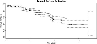
Turnbull survival curve, taking interval‐censoring into account.

In our analysis, 12 potential prognostic factors were included in the model, both in the latency and in the incidence part : Mini‐Mental State Examination (MMSE), expression, remote memory, learning, attention, praxis, abstract thinking, perception, ApoE4 status, gender, age, and years of total education, resulting in a total of 26 parameters. We used the EGG‐AFT cure mixture model to obtain unpenalized maximum likelihood estimates and the adaptive LASSO procedure described in Section 3 to perform variable selection.

Table 10 shows the adaptive LASSO estimate, the standard error estimated using formula from Section (3.3), and the exponentiated estimates. This allows a direct interpretation of the impact of covariates, in terms of acceleration or deceleration of the time to the event in latency and in terms of increase or decrease in odds for the incidence.

Table 10.

MCI results: adaptive LASSO estimates, standard errors, and exponentiated estimates.

	Parameter	aLASSO	SD	Exp(Estimate)
Latency	Intercept (Lat.)	2,628	0,155
	MMSE	—	—
	Expression	0,321	0,077	1,38
	Remote	—	—
	Learning	—	—
	Attention	−0,057	0,043	0,94
	Praxis	—	—
	Abstract thinking	0,086	0,034	1,09
	Perception	0,182	0,052	1,20
	ApoE4	−0,092	0,025	0,91
	Gender	−0,061	0,022	0,94
	Age (5y.)	−0,321	0,144	0,73
	Total education	0,152	0,163	1,16
Incidence	Intercept (Inc.)	2,657	0,985
	MMSE	−2,250	0,802	0,11
	Expression	—	—
	Remote	—	—
	Learning	−0,969	0,425	0,38
	Attention	—	—
	Praxis	−1,302	0,564	0,27
	Abstract thinking	0,483	0,456	1,62
	Perception	—	—
	ApoE	−0,556	0,264	0,57
	Gender	—	—
	Age (5y.)	—	—
	Total education	2,285	2,081	9,83

MCI, mild cognitive impairment; MMSE, Mini‐Mental State Examination; ApoE E4, Apolipoprotein E4.

Last column gives the increase in time‐to‐the‐event (for the latency) and odds ratio (for incidence).

Focusing on susceptible people (the latency part), there are three variables increasing the expected duration, thus, having a positive impact on the survival, by at least 15%: Expression (38%), Perception (20%) and Education (16%). On the other hand, only the age shortens the duration by at least 15%: When age increases by 5 years, the expected time until conversion is shorten by 27%. For comparison, without considering cure, the perception score was not significant, whereas the learning score was significant, with a positive impact on the survival. However, we see that learning still has a positive impact, but in the incidence part, reducing the risk to be susceptible. Three other variables have a positive impact on the probability to be susceptible: MMSE (−89%), praxis (−73%), ApoE4 status (−43%). At the opposite, the abstract thinking (62%) and the total years of education (883%) have here a highly negative impact and significantly increases the odds ratio.

With these results, we estimated the average cure proportion in the whole sample to 20%. Analyzing these data taking a cure fraction into account leads to more information: first, the positive impact of the learning variable is now due to the fact that it reduces the probability to convert to MCI. Second, we now consider other variables that have an impact: those impacting the probability to experience the disease.

6. Conclusion and Discussion

In this article, we consider the AFT model in a context where data are interval censored and where a fraction of the population is not susceptible or cured from the event of interest. In survival analysis, the Cox proportional hazards model is widely used, provided that the proportional hazards assumption is met. Typically, in these cases, survival curves do not cross with each other. In the presence of a cure fraction, even if the survival distribution for susceptibles truly comes from a PH model, curves can cross with each other 21. To our knowledge, there is no method to distinguish crossing hazards that are due to the presence of cure from crossing hazards that are due to a true non‐proportionality in the latency. Using an AFT model circumvents this issue in addition of providing a straightforward interpretation of the results.

Parametric models are often criticized because a departure from the true underlying distribution can have substantial consequences. Nonetheless, in the presence of interval‐censoring and cure, it is very difficult to develop simple yet efficient estimation procedures without imposing parametric restrictions. This is why a flexible distribution, capable of capturing a lot of characteristics, is an excellent compromise in this context.

Although widely used in the context of dimension reduction, when the number of covariates exceeds the number of observations, shrinkage methods are also useful in our context. Indeed, the number of covariates may be large, as a set of covariates can be included twice, that is, in both parts of the model. This is why we believe that such shrinkage methods should be extended to the mixture cure model.

Different aspects were highlighted from the simulation studies. First, using a mixture cure model, when a cure fraction is truly present, reduces the bias in the latency part. Second, if sample size is small and if there are not enough cured individuals compared with the right‐censoring proportion, then the bias and MSE in the incidence part can be large. Thus, there is a trade‐off between the gain in bias in the latency and the instability of estimates in the incidence. It is clear that if not enough cured individuals are present in the database, the model will not be able to discriminate between the susceptible and cured ones. Also, making use of the mixture cure model results in a different interpretation. Covariates can have an impact on the survival, on the cure probability, or on both. This leads to even more information about the event of interest.

In conclusion, our model and variable selection procedure offers flexibility as well as an easy way to interpret the results. Even more flexibility can be reached, and other variable selection procedures deserve more attention in parametric cure mixture models. Those are subject to future work.

Supporting information

Supporting Info Item

Scolas, S. , El Ghouch, A. , Legrand, C. , and Oulhaj, A. (2016) Variable selection in a flexible parametric mixture cure model with interval‐censored data. Statist. Med., 35: 1210–1225. doi: 10.1002/sim.6767.

References

- 1. Collie A, Maruff P, Shafiq‐Antonacci R, Smith M, Hallup M, Schofield PR, Masters CL, Currie J. Memory decline in healthy older people: implications for identifying mild cognitive impairment. Neurology 2001; 56(11):1533–1538. [DOI] [PubMed] [Google Scholar]
- 2. De Jager C, Blackwell AD, Budge MM, Sahakian BJ. Predicting cognitive decline in healthy older adults. American Journal of Geriatric Psychiatry 2005; 13(8):735–740. [DOI] [PubMed] [Google Scholar]
- 3. Weaver Cargin J, Collie A, Masters C, Maruff P. The nature of cognitive complaints in healthy older adults with and without objective memory decline. Journal of Clinical and Experimental Neuropsychology 2008; 30(2):245–257. [DOI] [PubMed] [Google Scholar]
- 4. Oulhaj A, Wilcock GK, Smith AD, de Jager CA. Predicting the time of conversion to MCI in the elderly: role of verbal expression and learning. Neurology 2009; 73(18):1436–1442. [DOI] [PMC free article] [PubMed] [Google Scholar]
- 5. Petersen RC, Doody R, Kurz A, Mohs RC, Morris JC, Rabins PV, Ritchie K, Rossor M, Thal L, Winblad B. Current concepts in mild cognitive impairment. Archives of Neurology 2001; 58(12):1985–1992. [DOI] [PubMed] [Google Scholar]
- 6. Gomez G, Calle ML, Oller R, Langohr K. Tutorial on methods for interval‐censored data and their implementation in R. Statistical Modelling 2009; 9(4):259–297. [Google Scholar]
- 7. Turnbull BW. The empirical distribution function with arbitrarily grouped, censored and truncated data. Journal of the Royal Statistical Society. Series B (Methodological) 1976; 38(3):290–295. [Google Scholar]
- 8. Dehghan M, Duchesne T. A generalization of turnbull's estimator for nonparametric estimation of the conditional survival function with interval‐censored data. Lifetime Data Analysis 2011; 17(2):234–255. [DOI] [PubMed] [Google Scholar]
- 9. Finkelstein DM, Wolfe RA. A Semiparametric Model for Regression Analysis of Failure Time Data. Biometrics 1985; 41(4):933–945. [PubMed] [Google Scholar]
- 10. Rabinowitz D, Tsiatis A, Aragon J. Regression with interval‐censored data. Biometrika 1995; 82(3):501–513. [Google Scholar]
- 11. Pan W. Extending the iterative convex minorant algorithm to the cox model for interval‐censored data. Journal of Computational and Graphical Statistics 1999; 8(1):109–120. [Google Scholar]
- 12. Komárek A, Lesaffre E, Hilton JF. Accelerated failure time model for arbitrarily censored data with smoothed error distribution. Journal of Computational and Graphical Statistics 2005; 14(3):726–745. [Google Scholar]
- 13. Sun J. The Statistical Analysis of Interval‐Censored Failure Time Data, Statistics for Biology and Health Springer: New York, 2006. [Google Scholar]
- 14. Chen D, Sun J, Peace K. Interval‐Censored Time‐to‐Event Data: Methods and Applications. Chapman & Hall/CRC: London, 2012. [Google Scholar]
- 15. Dempster AP, Laird NM, Rubin DB. Maximum likelihood from incomplete data via the EM algorithm. Journal of the Royal Statistical Society Series B (Methodological) 1977; 39(1):1–38. [Google Scholar]
- 16. Boag J. Maximum likelihood estimates of the proportion of patients cured by cancer therapy. Journal of the Royal Statistical Society. Series B (Methodological) 1949; 11(1):15–53. [Google Scholar]
- 17. Berkson J, Gage R. Survival curve for cancer patients following treatment. Journal of the American Statistical Association 1952; 47(259):501–515. [Google Scholar]
- 18. Tsodikov A. A proportional hazards model taking account of long‐term survivors. Biometrics 1998; 54(4):1508–1516. [PubMed] [Google Scholar]
- 19. Tsodikov A, Ibrahim J, Yakovlev A. Estimating cure rates from survival data: an alternative to two‐component mixture models. Journal of the American Statistical Association 2003; 98: 1063–1078. [DOI] [PMC free article] [PubMed] [Google Scholar]
- 20. Taylor JMG. Semiparametric estimation in failure time mixture models estimation. Biometrics 1995; 51(3):899–907. [PubMed] [Google Scholar]
- 21. Sy JP, Taylor JMG, Way DNA, Francisco SS. Estimation in a Cox proportional hazard cure model. Biometrics 2000; 56(1):227–236. [DOI] [PubMed] [Google Scholar]
- 22. Peng Y, Dear KBG. A nonparametric mixture model for cure rate estimation. Biometrics 2000; 56(1):237–243. [DOI] [PubMed] [Google Scholar]
- 23. Li CS, Taylor JMG. A semi‐parametric accelerated failure time cure model. Statistics in Medicine 2002; 21(21):3235–3247. [DOI] [PubMed] [Google Scholar]
- 24. Zhang J, Peng Y. A new estimation method for the semiparametric accelerated failure time mixture cure model. Statistics in Medicine 2007; 26: 3157–3171. [DOI] [PubMed] [Google Scholar]
- 25. Farewell VT. The combined effect of breast cancer risk factors. Cancer 1977; 40(2):931–936. [DOI] [PubMed] [Google Scholar]
- 26. Wei L. The accelerated failure time model: a useful alternative to the Cox regression model in survival analysis. Statistics in Medicine 1992; 11: 1971–1879. [DOI] [PubMed] [Google Scholar]
- 27. Reid N. A conversation with sir david cox. Statistical Science 1994. 08; 9(3):439–455. [Google Scholar]
- 28. Yamaguchi K. Accelerated failure‐time regression models with a regression model of surviving fraction: an application to the analysis of “permanent employment”? in Japan. Journal of the American Statistical Association 1992; 87(418):284–292. [Google Scholar]
- 29. Chen C‐H, Tsay Y, Wu Y, Horng C. Logistic AFT location‐scale mixture regression models with nonsusceptibility for left‐truncated and general interval‐censored data. Statistics in Medicine 2013; 32(24):4285–4305. [DOI] [PubMed] [Google Scholar]
- 30. Fan J, Li R. Variable selection via nonconcave penalized likelihood and its oracle properties. Journal of the American Statistical Association 2001; 96(456):1348–1360. [Google Scholar]
- 31. Harrell F. Regression Modeling Strategies: With Applications to Linear Models, Logistic Regression, and Survival Analysis, Graduate Texts in Mathematics Springer: New‐York, 2001. [Google Scholar]
- 32. Tibshirani R. Regression shrinkage and selection via the lasso. Journal of the Royal Statistical Society. Series B(Methodological) 1996; 58(1):267–288. [Google Scholar]
- 33. Zou H. The adaptive lasso and its oracle properties. Journal of the American Statistical Association 2006; 101(476):1418–1429. [Google Scholar]
- 34. Efron B, Hastie T. Least angle regression. The Annals of Statistics 2004; 32(2):407–499. [Google Scholar]
- 35. Friedman J, Hastie T. Pathwise coordinate optimization. The Annals of Applied Statistics 2007; 1(2):302–332. [Google Scholar]
- 36. Liu X, Peng Y, Tu D, Liang H. Variable selection in semiparametric cure models based on penalized likelihood, with application to breast cancer clinical trials. Statistics in Medicine 2012; 31(24):2882– 2891. [DOI] [PubMed] [Google Scholar]
- 37. Lawless JF. Inference in the generalized gamma and log gamma distributions. Technometrics 1980; 22(3):409–419. [Google Scholar]
- 38. Stacy E. A generalization of the gamma distribution. The Annals of Mathematical Statistics 1962; 33(3):1187–192. [Google Scholar]
- 39. Prentice RL. A log gamma model and its maximum likelihood estimation. Biometrika 1974; 61(3):539–544. [Google Scholar]
- 40. Li CS, Taylor JMG, Sy JP. Identifiability of cure models. Statistics & Probability Letters 2001; 54(4):389–395. [Google Scholar]
- 41. Hanin L, Huang LS. Identifiability of cure models revisited. Journal of Multivariate Analysis 2014; 130: 261–274. [Google Scholar]
- 42. Peng Y, Dear KBG, Denham JW. A generalized F mixture model for cure rate estimation. Statistics in Medicine 1998; 17: 813–830. [DOI] [PubMed] [Google Scholar]
- 43. Hoerl AE, Kennard RW. Ridge regression: applications to nonorthogonal problems. Technometrics 1970; 12: 69–82. [Google Scholar]
- 44. Zhang HH, Lu W. Adaptive lasso for Cox's proportional hazards model. Biometrika 2007; 94(3):691–703. [Google Scholar]
- 45. Wang H, Leng C. Unified LASSO estimation by least squares approximation. Journal of the American Statistical Association 2007; 102(479):1039–1048. [Google Scholar]
- 46. Lu W, Zhang HH. Variable Selection for Linear Transformation Models via Penalized Marginal Likelihood, Institute of Statistics Mimeo Series 2580 North Carolina State University: Rayleigh, 2006. [Google Scholar]
- 47. Corder E, Saunders AM, Strittmatter WJ, Schmechel DE, Gaskell PC, Small GW, Roses AD, Haines JL, Pericak‐Vance MA. Gene dose of apolipoprotein e type 4 allele and the risk of Alzheimer's disease in late onset families. Science 1993; 261: 921–923. [DOI] [PubMed] [Google Scholar]
Associated Data
This section collects any data citations, data availability statements, or supplementary materials included in this article.
Supplementary Materials