MR fingerprinting with simultaneous B1 estimation

Abstract

Purpose

MR fingerprinting (MRF) can be used for quantitative estimation of physical parameters in MRI. Here, we extend the method to incorporate B1 estimation.

Methods

The acquisition is based on steady state free precession MR fingerprinting with a Cartesian trajectory. To increase the sensitivity to the B1 profile, abrupt changes in flip angle were introduced in the sequence. Slice profile and B1 effects were included in the dictionary and the results from two‐ and three‐dimensional (3D) acquisitions were compared. Acceleration was demonstrated using retrospective undersampling in the phase encode directions of 3D data exploiting redundancy between MRF frames at the edges of k‐space.

Results

Without B1 estimation, T2 and B1 were inaccurate by more than 20%. Abrupt changes in flip angle improved B1 maps. T1 and T2 values obtained with the new MRF methods agree with classical spin echo measurements and are independent of the B1 field profile. When using view sharing reconstruction, results remained accurate (error <10%) when sampling under 10% of k‐space from the 3D data.

Conclusion

The methods demonstrated here can successfully measure T1, T2, and B1. Errors due to slice profile can be substantially reduced by including its effect in the dictionary or acquiring data in 3D. Magn Reson Med 76:1127–1135, 2016. © 2015 The Authors Magnetic Resonance in Medicine published by Wiley Periodicals, Inc. on behalf of International Society for Magnetic Resonance in Medicine. This is an open access article under the terms of the Creative Commons Attribution‐NonCommercial‐NoDerivs License, which permits use and distribution in any medium, provided the original work is properly cited, the use is non‐commercial and no modifications or adaptations are made.

INTRODUCTION

Physical properties of tissue contributing to MRI signal are significantly modified by disease. Quantitative changes in longitudinal (T1) and transverse (T2) relaxation times in discrete brain regions have been described in a host of different pathologies 1. However, reproducibility for quantitative MRI measurements has proved a challenge and requires lengthy scan times to obtain parameters sequentially. Consequently, quantitative parameters are rarely acquired, and most evaluations of MRI images are based on visual inspection without quantitative evaluation of underlying values of T1 and T2.

Recently, a new approach of estimating multiple parameters at once, called MR fingerprinting (MRF), has been proposed 2. This method has the potential to be used for quantitative MRI routinely in both clinical and preclinical environments, enabling new tools for research and diagnosis. MR fingerprinting is based on the response of tissues to repeated acquisition sequences without attaining the steady state. Voxel‐wise responses are compared with a dictionary of simulated responses calculated from particular parameters (including, but not limited to, T1 and T2) and voxels are assigned the parameters from the best match to produce multiparametric maps.

To date, MRF has been performed with fast gradient echo sequences based on steady state free precession (SSFP). For fully rewound sequences, the simulations for the fingerprint database must include an estimate of the voxel‐wise frequency inhomogeneity for the correct signal evolution 2. Estimates of frequency offsets are not required for gradient‐spoiled sequences 3. MRF methods have also been demonstrated in preclinical scanning of rodents 4. To apply the technique of MRF in small animals, where less B0 homogeneity is usually achieved, a gradient‐spoiled approach has been used.

Due to data redundancy between frames, MRF is well‐suited to acceleration by means of undersampling. When undersampling with a pseudorandom scheme, acquisitions are affected by noise‐like aliasing. The MRF technique has been shown to be remarkably robust to aliasing 2. This characteristic can be used to achieve alias‐free maps in short times. However, anti‐aliasing the MRI images before MRF pattern recognition is also possible 5, 6. Here, we tested a reconstruction method with a simple anti‐aliasing technique, sharing the edges of k‐space between neighboring MRF frames before comparing signal evolution traces with the fingerprint database.

Current MRF methods, both in the clinical and preclinical environment, have been demonstrated assuming a perfectly rectangular slice profile and homogeneous excitation. However, these assumptions are violated in most practical MRI experiments. Indeed, it has been shown that different pulse shapes used for slice selection produce different T2 values 4. In addition, inhomogeneous radiofrequency excitation profiles are a common problem in both preclinical and clinical high‐field scanners.

We have extended the MRF approach by including a parameter for B1 in the signal evolution dictionary. In addition, we have implemented a three‐dimensional (3D) acquisition and tested a new anti‐aliasing strategy applied before pattern recognition. The 3D acquisition has the advantage of broader coverage (particularly important for whole brain imaging) and the considerable reduction of slice profile effects. As well as B1 estimation, we incorporated slice profile correction into the MRF reconstruction algorithm. All of these advances are demonstrated in a rodent head using a small‐bore scanner.

METHODS

MRF Acquisition

Our scheme builds on SSFP MRF as recently reported 3. Briefly, an inversion pulse is applied before a train of fast imaging with steady state precession readouts with variable flip angles and repetition time delays. These rapid changes prevent a steady state from being achieved, but rather lead to signal variations dependent on local magnetic properties and the applied B1 field. Phase encoding is applied before each readout and rewound afterward so that each train of readouts has the same phase encoding value and the whole sequence is repeated for each phase encoding step. In our implementation, we used a train of 1000 frames taking 10 s to acquire a single k‐line for all frames. To allow for return to equilibrium, we inserted a delay of 5 s before repeating the acquisition with a different level of phase encoding.

To increase the sensitivity to different B1 values, we changed the final part of the sequence from the original MRF approach as shown in Figure 1. By using abrupt changes of the nominal excitation flip angle, our scheme introduces oscillations of signal the frequency of which is proportional to the obtained flip angle (Fig. 2), and independent from T2. This phenomenon has been previously described to perform B1 mapping using SSFP sequences 7. We used alternating blocks of 15 pulses of flip angle 90° followed by 15 pulses of flip angle 0° to exploit the oscillatory behavior of the signal to resolve the B1 field.

Figure 1.

SSFP MRF schemes. A: the TR pattern used in all acquisitions. B: The FA pattern from the original SSFP MRF paper. C: The modified FA pattern demonstrated here, including abrupt changes in flip angle to increase the sensitivity to the B1 field.

Figure 2.

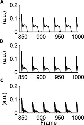
Simulation of the signal obtained with our novel MRF scheme (T1 = 160 ms T2 = 44 ms) at the end of the MRF train, in correspondence with abrupt changes in flip‐angle. Flip angle changes between blocks of 45° and 0° (A), between 90° and 0°(B), between 135° and 0°(C).

Phantom Experiments

Two different phantoms were used, one to investigate 2D MRF and another to assess the accuracy of the measurements across partitions of a 3D acquisition. First, we investigated 2D MRF. We imaged agarose gel samples with different T1s and T2s. We used a Bruker BioSpec 47/40 system (Bruker Inc., Ettlingen, Germany) equipped with 400 mT/m gradients and a 12 cm diameter quadrature birdcage coil used as a transceiver. We used sinc pulse of 2 ms for excitation. Each signal acquisition was preceded by an adiabatic inversion pulse (15 ms hyperbolic secant). MRF acquisitions were performed at the magnet isocenter on a single slice (3 mm slice thickness; field of view 7 cm; 64 × 64 matrix yielding 1.1 mm resolution with 50 kHz receiver bandwidth).

To assess 3D MRF acquisitions, we used a matrix of 64 × 64 × 64 for 0.5 mm isotropic resolution of a uniform gel with a T1 of 640 ms and a T2 of 74 ms. We measured the average value obtained in a region of interest through the slice direction (z). We compared the following methods: the original MRF method (with no B1 in the dictionary); the original MRF scheme including B1 in the dictionary; our new method with abrupt changes in flip angle; and classical methods (described below).

Brain Experiments

A formalin‐fixed Lister‐hooded adult rat brain was imaged using a 35‐mm‐diameter linear birdcage coil for both signal transmission and reception. For 2D MRF, we tried three different excitation pulse shapes: sinc, hermite, and gauss each of 2 ms and bandwidth factors 6.21, 5.40, and 2.74, respectively. Each slice had 0.5 mm thickness with a matrix of 64 × 64. For 3D acquisitions, we used a 64 × 64 × 64 matrix with 0.5 mm isotropic resolution (a 2 ms sinc excitation pulse as above was used).

As in the phantom acquisitions, each signal acquisition was preceded by an adiabatic inversion pulse (hyperbolic secant, length 15 ms, bandwidth factor 77.86). The receiver bandwidth was 50 kHz in each case.

Undersampling and Anti‐aliasing

The scan time for the fully sampled 3D acquisition was 17 h 4 min (10 s MRF train + 5 s recovery time) × (64 × 64) phase encoding steps. To test our acceleration strategy, we retrospectively undersampled the 3D acquisition of the ex vivo rat brain. Our undersampling scheme consisted of a binary mask in the phase encode directions (k_y‐k_z plane) as shown in Figure 3. Nonlinear sampling based on a Gaussian distribution around the k‐space center was used with a uniform angular distribution. The Gaussian function had a standard deviation of 45% of the full k_y and k_z axes. Masks were created independently for each image frame. This could be implemented readily on a scanner by acquiring a list of pre‐planned k‐lines varying for each frame.

Figure 3.

A: The undersampling scheme used for our accelerated 3D acquisitions acquiring 9% of k‐space. k‐Space was retrospectively undersampled in the phase encode directions ky and kz. B: The sampling density of k‐space with our undersampling method. C: The values corresponding to the k‐space location (32, 15, 15) for all frames when zero‐filling. D: k‐space data for the same location as (C) when using our view‐sharing method, applying a nearest‐neighbor interpolation through time.

We tested three different approaches for reconstructing the data. First, zero‐filling of the unsampled points was used. Second, zero‐filling was combined with density‐correction for the sampled regions. Here, the correction was obtained using the inverse of the sampling probability density function used for generating the k‐space masks. Finally, we implemented a view‐sharing strategy where unacquired k‐space points were borrowed from the nearest frame with an acquired point at that location. As a result of our sampling density, points closer to the center, containing most of the contrast information, were acquired with higher temporal resolution. On the other hand, the edges of k‐space, changing less during the MRF signal evolution, were acquired at lower temporal resolution.

To test our undersampling strategy we prepared multiparametric MRF maps using data from the fully sampled k‐space. We compared maps obtained from 18%, 9%, and 5% of k‐space to values found using the full dataset. Values were measured in the whole brain and muscle tissue, which were automatically masked using thresholding. The thresholding criterion was of a T1 between 0 and 1 s, which included all brain and muscle for our formalin‐fixed sample.

To perform a time‐matched comparison of our view sharing technique, we compared the use of only 8% of k‐space for all frames with fully acquiring only the first 80 frames of the MRF sequence. We compared root mean square errors relative with full sampling. For this experiment, aimed at evaluating the efficiency of the acquisition only, we excluded B1 from the dictionary.

MRF Reconstruction

Signal simulations were performed using extended phase graphs 8, including gradient de‐phasing as well as radiofrequency pulses and signal evolution. The pattern recognition reconstruction was implemented following 2. All code for simulation and pattern recognition was written in Matlab (Mathworks, Natick, MA). The dictionary contained values of T1 ranging from 80 ms to 1000 ms in steps of 20 ms, and from 1 to 2.5 s in steps of 50 ms. Values of T2 ranged from 10 ms to 100 ms in steps of 2 ms and from 105 ms to 250 ms in steps of 5 ms. B1 was modelled by a flip‐angle factor, a linear factor equal to the obtained flip angle divided by the desired flip angle. Values for this parameter were simulated from 50 to 150% in 2% increments.

Comparison with Classical Estimation of T1, T2, and B1

The quantitative maps using each scheme were compared with standard estimation of T1, T2 and B1 using manufacturer‐provided sequences. T1 and T2 were estimated using spin‐echo sequences with the same field of view (FOV) and matrix as the MRF acquisitions. The MRF scan times were compared with scan times from the manufacturer‐provided T1+T2 RARE relaxometry sequence, with unchanged sequence parameters [multiecho spin echo; echo time (TE): 11, 33, 55, 77, 99 ms; repetition time (TR) 200, 400, 800, 1500, 3000, 4500 ms; number of excitations (NEX), 1] on the same geometry. For more accuracy, in our classical measurements we increased the number of sampled points and averages and used single echoes rather than multiecho to reduce the impact of system imperfections. However, for comparison of the time taken we used the acquisition time of the unmodified sequence. T1 was estimated with a spin echo sequence with variable TR (TR: 10,000, 3000, 1500, 800, 400, 200 ms; TE: 11 ms; receiver bandwidth 48 kHz, 3 NEX). T2 was estimated with single‐echo spin‐echo acquisitions with variable TE (TR: 2500 ms; TE: 12, 36, 48, 60, 84, 108, 216, 324, 500 ms; receiver bandwidth 60 kHz, 1 NEX). The B1 field was estimated using the double‐angle method 7. Two gradient echo images were acquired with a flip angle of 45° and 90° on with the same FOV of the MRF acquisitions (TR/TE 15,000/2.9 ms, excitation with sinc pulse of 2 ms duration, receiver bandwidth 78 kHz, 1 NEX).

Slice Profile Correction for 2D MRF

Due to slice profile imperfections, the flip angle seen by spins varies across the slice and includes some contribution from spins outside the slice. To account for these effects in the MRF dictionary, a novel correction method was developed. The Shinnar‐Le Roux algorithm 15 was used to create a slice profile of 128 partitions based on the pulse waveforms used by the scanner. The extended phase graph simulation was performed for the central flip angle of each of the 128 partitions producing an MRF train for each. The signal of each frame was summed over each partition to create a dictionary for each pulse waveform that takes account of the variability in flip angles experienced across the slice. We compared MRF maps derived from slice‐profile corrected and the original dictionaries.

RESULTS

Reconstruction time for the parametric maps (including B1) from each slice was less than 1 min. Figure 4 compares estimates of T1, T2, and B1 from our acquisitions with the original MRF train of delays and flip angles, our modified scheme and the standard spin echo method. Good agreement was seen between techniques for T1 with less than 5% discrepancy between methods. We found that the previously reported MRF sequences did not successfully resolve T2 and B1 effects with substantial errors in the estimation of both. Our new method, as a result of abrupt changes in flip angle, was able to better discriminate between these parameters. However, this 2D MRF acquisition did not provide a complete separation of T2 and B1 due to slice profile effects, and B1 maps systematically underestimated (>10%) the true values when using a 2D acquisition.

Figure 4.

Results comparing the original MRF scheme, our modified scheme with abrupt changes in flip angle (dFA) and the maps using classical methods (described in methods). The original scheme confounds T2 and B1 effects, while scheme 2 can, though here with 2D acquisitions a systematic underestimation of B1 is seen relative to the double angle method.

The effect of slice profiles on MRF results is clear in Figure 5 which shows MRF maps from the rat brain without slice profile correction for sinc, hermite, and gauss pulses with 3D MRF and spin echo methods for comparison. As in the phantom, MRF‐derived T1 measurements do not appear to be sensitive to the slice profile but the estimates for T2 and B1 vary considerably. Compared with 3D for sinc, hermite, and gauss shapes, T1 values differ by 3.8%, 3.8%, and 4.3%; T2 values differ by 6.5%, 17%, and 8.7%, and B1 differs by 8.4%, 6.7%, and 36% (RMS errors).

Figure 5.

Comparison between 2D MRF with different slice profiles, our 3D MRF acquisition, and classical methods. When performing 2D imaging, only using a sinc excitation agreed with the 3D acquisition, despite a constant negative bias in B1. 3D MRF slightly underestimated both T1 and T2 compared with spin echo measurements, but agreed well with double‐angle B1 measurements.

The discrepancies in the B1 estimation are considerably reduced when slice profiles are taken into account (Fig. 6). The corresponding discrepancies for T1 values are 3.8%, 3.8%, and 4.6%; for T2 24%, 14.9%, and 7.7% and B1 4.0%, 2.6%, and 5.3% for sinc, hermite, and gauss shapes, respectively (RMS compared with 3D).

Figure 6.

Comparison between MRF results for T2 and B1 with and without slice profile correction (labeled SLR). The 3D measurements are also reported for comparison.

Figure 7 shows profile plots of T1, T2, and B1 measured from a uniform phantom with the original MRF approach, MRF with correction for B1 with and without the abrupt flip angle changes in addition to the standard measurements. T1 measurement is accurate for MRF methods across the slice, where the spin‐echo measurement is inaccurate away from the center. Without modeling B1 in the dictionary, MRF overestimates the T1 value. For T2 and B1, results are similar to Figure 4 with confounded estimates unless abrupt flip angle changes are introduced into the scheme.

Figure 7.

Quantitative measurements on a uniform phantom plotted through the 3D slice direction. Classical estimates of T1 and T2 were biased due to imperfect B1. The original MRF scheme with no B1 estimate (in blue) presented a bias dependent on B1. The original scheme including B1 estimation (dotted green) could not discriminate between T2 and B1 effects. Our new MRF acquisition including abrupt changes in flip‐angle (black, labelled dFA) had no significant bias, and compared well with the expected values (magenta). At the edges of the slice, some T2 underestimation can be observed.

Figure 8 compares the different approaches to deal with undersampled data, and it can be seen that view‐sharing significantly outperforms the other methods. A comparison of the view‐sharing method on 8% kspace with a time‐matched acquisition fully acquiring just the first 80 MRF frames revealed that spatial undersampling has a high efficiency. A view sharing method using only 8% of k‐space gave lower errors (ΔT1 = 35 ms; ΔT2 = 4 ms; RMS compared with full) than a time‐matched comparison using only the first 80 elements of the MRF sequence (ΔT1= 450 ms; ΔT2= 50 ms; RMS compared with full).

Figure 8.

Quantitative T1 maps from an axial slice of our multiparametric 3D MRF acquisition, comparing fully sampled data with maps obtained acquiring only 8% of k‐space. Zero filling generates artifacts due to nonuniform sampling of k‐space; density correction of the zero‐filled data recovers the details in the image but results in a noisy map; sharing k‐space points between neighboring time frames reduces the noise.

Acquisitions using 18% of k‐space (3 h long) and 9% of k‐space (1.5 h long), generated quantitative maps (Fig. 9) within 10% error of the fully sampled case. All the undersampled MRF scans were faster than the manufacturer‐provided T1+T2 RARE relaxometry sequence on the same geometry (4.5 h). Further acceleration factors still generated acceptable results. MRF maps from only 5% of k‐space are shown in Supporting Figure S1, which is available online. This corresponds to an acquisition of approximately 50 min for the whole brain. For this acquisition, some areas of the B1 and T2 maps presented errors superior to 10%, mostly in remote areas of the head where B1 is changing more rapidly and in areas with low SNR (e.g., due to the inclusion of air in the ex vivo sample).

Figure 9.

Comparison of a full 3D dataset of a fixed rat brain with the maps reconstructed using only 18% of the data and 9% of the data. The undersampled sets agree well with the fully sampled dataset.

Values for mean error due to undersampling, as well as 5% and 95% percentiles are reported in Table 1. Undersampling the acquisitions did not significantly bias the T1, T2, and B1 estimates.

Table 1.

Error of Undersampled Acquisitions with Respect to Full, Calculated on a Mask Including the Brain and Muscle^a

Error (full ‐ undersampled), mean [5% percentile ; 95% percentile]
	T1(ms)	T2(ms)	B1
18% k‐space	−1.8 [−40; 40]	0.9 [−7; 4]	0.003 [−0.04; 0.03]
9% k‐space	−6 [−60; 60]	−1.9 [−11;5]	−0.003 [−0.06; 0.05]
5% k‐space	−11 [−100; 80]	−3.2 [−18; 9]	0.0008 [−0.09; 0.1]

^aData are expressed as mean error [5% percentile; 95% percentile].

DISCUSSION

We have shown that B1 estimation can be used in an MRF framework and that this acquisition can be extended to 3D. This is particularly important for the application of MRF to small‐bore preclinical scanners where small RF coils may have significant inhomogeneity. The inclusion of B1 effects will be of growing importance, as these are problematic for body imaging at both 3T and 7T 10, 11 and brain imaging at 7T 12.

Images in MRF scans can be reconstructed from undersampled k‐space, as the MRF reconstruction “sees through” aliasing 2. However, anti‐aliasing strategies may permit higher undersampling factors. Here we have successfully demonstrated a simple strategy to deal with undersampled k‐space acquisitions. In our scheme, non‐acquired k‐space points in one frame are “borrowed” from neighboring frames where these had been acquired. This concept, similar to keyhole imaging 13, is based on the fact that the image contrast is mainly in the center of k‐space, while the image details, which are unchanged between frames, are in the edges of k‐space. Therefore, the signal evolution is estimated well when only the central part of k‐space is updated in subsequent frames.

When doing slice selective imaging, different locations in the slice are excited with a different flip angle leading to partial volume effects. In MRF, partial volume effects have a different behavior with respect to conventional imaging 14. In conventional imaging, different sub‐voxel areas are averaged within a voxel, while MRF tends more toward the most represented sub‐voxel area, as it can be noted when using different pulses in Figure 5, where B1 is not homogeneous throughout the voxel. We demonstrated that the slice profile can be directly included in the simulation, performing independent calculations for single sub‐voxel areas using slice profiles derived from the Shinnar‐Le Roux algorithm 15. Residual errors in T2 are likely due to nonideal behavior of the RF transmission pipeline. To check this, we used actual flip angle imaging 16 to measure the mean flip angle in a uniform phantom achieved when different pulse shapes were used. The measured flip angles were found to be factors of 1.07 for sinc, 1.06 for hermite, and 0.96 for gauss pulses. Introducing these factors for flip angles into the dictionary reduced the errors but further investigation of imperfect RF transmission was beyond the scope of this study.

The adverse effects of slice distortion can be largely mitigated when selecting a large slab for 3D imaging, as in this case the slice profile problem becomes part of the B1 estimation. When estimating parameters through the slice, we saw unbiased results with our new method. However, we still observed underestimation of T2 in the outermost partitions. Future acquisitions with non‐selective pulses could offer a better solution for an extended coverage. Previous work in the context of radial k‐space acquisition found that 3D scans offer more possibility of undersampling the k‐space with respect to 2D slices 17. Another advantage of 3D imaging is its applicability to brain imaging cohort studies. Brain imaging methods to compare groups of subjects usually benefit from isotropic 3D acquisitions to meaningfully compare regions after image registration 18. In addition, whole‐brain coverage can be achieved in a single acquisition when using 3D MRF methods.

By accelerating the acquisition more than 10‐fold, our method is significantly faster than MRF protocols currently available for small animals 4. The undersampling technique described here can be used to significantly shorten scan times, and achieve acquisition durations suitable for in vivo imaging of rodents. Current techniques for voxel‐wise comparison of rodent brains include voxel‐based morphometry 19 and tensor‐based morphometry 20. However, both approaches are more concerned with image geometry rather than the signal levels seen, as a consistent wide‐spread approach for quantitative imaging between centers has not appeared to date in the literature. Fully quantitative, 3D acquisitions could be used in this context to obtain standardized multicenter data for analysis of different disease models and treatments.

The scan times obtained here, of the order of 1.5 h, can be used in the preclinical environment, however, they would be prohibitive in human studies. The efficiency of our method is limited when compared with the gold standard of human quantitative imaging featuring acceleration with compressed sensing and parallel imaging. The introduction of array coils, as well as more sophisticated anti‐aliasing strategies, could be used to further accelerate MRF acquisitions. Using iterative reconstruction such as compressed sensing is a promising strategy for anti‐aliasing the images before pattern recognition 5, 6. However, the large size of 4D datasets represents a challenge for iterative algorithms, and new strategies are needed to deal with the high computational demand. For instance, new compressed sensing algorithms based on fast, dedicated processing units of high‐performance graphics cards (GPUs) developed for cardiac MRI hold promise for reconstruction of large MRF datasets 17. In addition, fast algorithms such as split Bregman could be used to accelerate compressed sensing of large datasets 21, perhaps including spatiotemporal total variation constraints 22.

In the current implementation, we waited for full relaxation (5 × T1) between acquiring k‐space lines. However, this is not necessary to perform MRF. In the future, optimized MRF acquisitions could be used to further shorten scan times. In addition, non‐Cartesian methods have been demonstrated in the preclinical environment as well as for clinical scanners. Non‐Cartesian acquisitions yield better efficiency and anti‐aliasing of undersampled data with respect to Cartesian in several preclinical applications, e.g., Buonincontri et al 23. MR fingerprinting has already been demonstrated using arbitrary gradient waveforms, for instance derived from music to increase patient's comfort 24. Although the use of spiral trajectories has shown great speed benefits for MRF in clinical scanners, we are unaware of implementations of spiral MRF in small‐bore MRI scanners. The use of novel 3D non‐Cartesian strategies could further accelerate the acquisition bringing 3D, isotropic MRF methods into both preclinical and clinical applications. Direct reductions in scan time can also be achieved by reducing the number of frames 25.

Including the slice profile correction increased the computational burden of the dictionary creation proportionally to the number of partitions used. However, this correction had no impact on the pattern recognition algorithm, as the dictionary size remained unchanged. It took approximately a minute per slice to reconstruct the MRF data here, and this is a reasonable time frame. It is possible to include further parameters in the reconstruction though this is prohibitive as the reconstruction time will scale exponentially with the number of parameters. Reconstruction times and memory occupancy represent the largest current limitation of MRF. New methods to meaningfully compress the dictionary 26 and perform more sophisticated matching 27 are currently being studied. New reconstruction methods could permit the measurement of more parameters simultaneously, such as T2* and diffusion, enhancing the sensitivity of novel MRF techniques.

CONCLUSIONS

We have demonstrated a method for incorporating B1 estimation into MRF and extended the protocol to 3D imaging. Our methods greatly reduced problems seen with particular pulse shapes and B1 inhomogeneity, improving the accuracy of parameters estimated from MRF. We showed that view sharing between MRF frames produces accurate results acquiring less than 10% of the full dataset.

Supporting information

Supporting Figure S1. Performance of 3D MRF acquiring only 5% of k‐space per frame (50 min), compared with full acquisition (17 h). Some sparse areas of the T2 and B1 maps have errors between 10 and 20% compared with the full acquisition.

REFERENCES

- 1. Deoni SC. Quantitative relaxometry of the brain. Top magn reson imaging 2010;21:101–113. [DOI] [PMC free article] [PubMed] [Google Scholar]
- 2. Ma D, Gulani V, Seiberlich N, Liu K, Sunshine JL, Duerk JL, Griswold MA. Magnetic resonance fingerprinting. Nature 2013;495:187–192. [DOI] [PMC free article] [PubMed] [Google Scholar]
- 3. Jiang Y, Ma D, Seiberlich N, Gulani V, Griswold MA. MR fingerprinting using fast imaging with steady state precession (FISP) with spiral readout. Magn Reson Med 2015;74:1621–1631. [DOI] [PMC free article] [PubMed] [Google Scholar]
- 4. Gao Y, Chen Y, Ma D, et al. Preclinical MR fingerprinting (MRF) at 7 T: effective quantitative imaging for rodent disease models. NMR Biomed 2015;28:384–394. [DOI] [PMC free article] [PubMed] [Google Scholar]
- 5. Davies M, Puy G, Vandergheynst P, Wiaux Y. A compressed sensing framework for magnetic resonance fingerprinting. Siam J Imaging Sci 2014;7:2623–2656. [Google Scholar]
- 6. Wang Z, Zhang Q, Yuan J, Wang X. MRF denoising with adaptive filtering. 2014. arXiv:1401.0670.
- 7. Ganter C, Settles M, Dregely I, Santini F, Scheffler K, Bieri O. B1+‐mapping with the transient phase of unbalanced steady‐state free precession. Magn Reson Med 2013;70:1515–1523. [DOI] [PubMed] [Google Scholar]
- 8. Weigel M. Extended phase graphs: dephasing, RF pulses, and echoes ‐ pure and simple. J Magn Reson Imaging 2015;41:266–295. [DOI] [PubMed] [Google Scholar]
- 9. Cunningham CH, Pauly JM, Nayak KS. Saturated double‐angle method for rapid B1+ mapping. Magn Reson Med 2006;55:1326–1333. [DOI] [PubMed] [Google Scholar]
- 10. Vaughan JT, Snyder CJ, DelaBarre LJ, Bolan PJ, Tian J, Bolinger L, Adriany G, Andersen P, Strupp J, Ugurbil K. Whole‐body imaging at 7T: preliminary results. Magn Reson Med 2009;61:244–248. [DOI] [PMC free article] [PubMed] [Google Scholar]
- 11. Bernstein MA, Huston J III, Ward HA. Imaging artifacts at 3.0T. J Magn Reson Imaging 2006;24:735–746. [DOI] [PubMed] [Google Scholar]
- 12. Vaughan JT, Garwood M, Collins CM, et al. 7T vs. 4T: RF power, homogeneity, and signal‐to‐noise comparison in head images. Magn Reson Med 2001;46:24–30. [DOI] [PubMed] [Google Scholar]
- 13. van Vaals JJ, Brummer ME, Dixon WT, Tuithof HH, Engels H, Nelson RC, Gerety BM, Chezmar JL, den Boer JA. “Keyhole” method for accelerating imaging of contrast agent uptake. J Magn Reson Imaging 1993;3:671–675. [DOI] [PubMed] [Google Scholar]
- 14. Deshmane AV, Ma D, Jiang Y, Fisher E, Seiberlich N, Gulani V, Griswold M. Validation of tissue characterization in mixed voxels using MR fingerprinting. In Proceedings of the 22nd Annual Meeting of ISMRM, Milan, Italy, 2014. Abstract 0094.
- 15. Pauly J, Le Roux P, Nishimura D, Macovski A. Parameter relations for the Shinnar‐Le Roux selective excitation pulse design algorithm [NMR imaging]. IEEE Trans Med Imaging 1991;10:53–65. [DOI] [PubMed] [Google Scholar]
- 16. Yarnykh VL. Actual flip‐angle imaging in the pulsed steady state: a method for rapid three‐dimensional mapping of the transmitted radiofrequency field. Magn Reson Med 2007;57:192–200. [DOI] [PubMed] [Google Scholar]
- 17. Nam S, Akcakaya M, Basha T, Stehning C, Manning WJ, Tarokh V, Nezafat R. Compressed sensing reconstruction for whole‐heart imaging with 3D radial trajectories: a graphics processing unit implementation. Magn Reson Med 2013;69:91–102. [DOI] [PMC free article] [PubMed] [Google Scholar]
- 18. Ashburner J, Friston KJ. Voxel‐based morphometry‐‐the methods. Neuroimage 2000;11(Pt 1):805–821. [DOI] [PubMed] [Google Scholar]
- 19. Sawiak SJ, Wood NI, Williams GB, Morton AJ, Carpenter TA. Voxel‐based morphometry with templates and validation in a mouse model of Huntington's disease. Magn Reson Imaging 2013;31:1522–1531. [DOI] [PMC free article] [PubMed] [Google Scholar]
- 20. Kielar C, Sawiak SJ, Navarro Negredo P, Tse DH, Morton AJ. Tensor‐based morphometry and stereology reveal brain pathology in the complexin1 knockout mouse. PloS One 2012;7:e32636. [DOI] [PMC free article] [PubMed] [Google Scholar]
- 21. Goldstein T, Osher S. The Split Bregman Method for L1‐regularized problems. Siam J Imaging Sci 2009;2:323–343. [Google Scholar]
- 22. Montesinos P, Abascal JF, Cusso L, Vaquero JJ, Desco M. Application of the compressed sensing technique to self‐gated cardiac cine sequences in small animals. Magn Reson Med 2014;72:369–380. [DOI] [PubMed] [Google Scholar]
- 23. Buonincontri G, Methner C, Krieg T, Carpenter TA, Sawiak SJ. Functional assessment of the mouse heart by MRI with a 1‐min acquisition. NMR Biomed 2014;27:733–737. [DOI] [PubMed] [Google Scholar]
- 24. Ma D, Pierre EY, Jiang Y, Schluchter MD, Setsompop K, Gulani V, Griswold MA. Music‐based magnetic resonance fingerprinting to improve patient comfort during MRI examinations. Magn Reson Med 2016;75:2303–2314. [DOI] [PMC free article] [PubMed] [Google Scholar]
- 25. Hamilton JI, Wright KL, Jiang Y, Hernandez‐Garcia L, Ma D, Griswold M, Sieberlich N. Pulse sequence optimization for improved MRF scan efficiency. In Proceedings of the 23rd Annual Meeting of ISMRM, Toronto, Canada, 2015. Abstract 3386.
- 26. McGivney DF, Pierre E, Ma D, Jiang Y, Saybasili H, Gulani V, Griswold MA. SVD compression for magnetic resonance fingerprinting in the time domain. IEEE Trans Med Imaging 2014;33:2311–2322. [DOI] [PMC free article] [PubMed] [Google Scholar]
- 27. Cauley SF, Setsompop K, Ma D, Jiang Y, Ye H, Adalsteinsson E, Griswold MA, Wald LL. Fast group matching for MR fingerprinting reconstruction. Magn Reson Med 2015;74:523–528. [DOI] [PMC free article] [PubMed] [Google Scholar]
Associated Data
This section collects any data citations, data availability statements, or supplementary materials included in this article.
Supplementary Materials