Abstract
Recent work on both task-induced and resting-state functional magnetic resonance imaging (fMRI) data suggests that functional connectivity may fluctuate, rather than being stationary during an entire scan. Most dynamic studies are based on second-order statistics between fMRI time series or time courses derived from blind source separation, e.g., independent component analysis (ICA), to investigate changes of temporal interactions among brain regions. However, fluctuations related to spatial components over time are of interest as well. In this paper, we examine higher-order statistical dependence between pairs of spatial components, which we define as spatial functional network connectivity (sFNC), and changes of sFNC across a resting-state scan. We extract time-varying components from healthy controls and patients with schizophrenia to represent brain networks using independent vector analysis (IVA), which is an extension of ICA to multiple data sets and enables one to capture spatial variations. Based on mutual information among IVA components, we perform statistical analysis and Markov modeling to quantify the changes in spatial connectivity. Our experimental results suggest significantly more fluctuations in patient group and show that patients with schizophrenia have more variable patterns of spatial concordance primarily between frontoparietal, cerebellum and temporal lobe regions. This study extends upon earlier studies showing temporal connectivity differences in similar areas on average by providing evidence that the dynamic spatial interplay between these regions is also impacted by schizophrenia.
Keywords: dynamic spatial change, spatial functional network connectivity, independent vector analysis, fMRI, schizophrenia
1. Introduction
A very active research topic in functional magnetic resonance imaging (fMRI) studies has been study of functional connectivity—statistical interactions among brain regions during cognitive or sensorimotor tasks, or merely from spontaneous activity during rest. Dysconnectivity or abnormal connectivity has typically been considered a hallmark of various mental disorders, especially schizophrenia (Bullmore et al., 1997; Stephan et al., 2009). Schizophrenia is still one of the most complex and heterogeneous mental disorders that impairs multiple cognitive domains including memory, attention, language, and execution function (Danielyan and Nasrallah, 2009; van Os and Kapur, 2009). Previous neuroimaging studies have found both structural and functional abnormalities in temporal lobe, parietal cortex, and cerebellum regions for schizophrenia (Iritani, 2007). Also, evidence of dysconnectivity among a number of brain networks in schizophrenia has been reported (Meyer-Lindenberg et al., 2001; Jafri et al., 2008; Yu et al., 2011; Jones et al., 2012). Most connectivity studies use independent component analysis (ICA), a popular data-driven method, to reveal robust markers for schizophrenia biomarkers. ICA separates single-subject fMRI data into a set of maximally independent components and associated time courses (McKeown et al., 1998; Calhoun et al., 2001a). Spatial components represent temporally coherent brain networks, and functional connectivity among these networks—called functional network connectivity—is typically defined as the correlation or coherence between associated time courses (Jafri et al., 2008; Allen et al., 2011a). An advantage of using ICA-based methods for functional connectivity analysis is that no explicit prior knowledge about brain activity is required and the estimates are not biased due to selection of a seed region of interest. For multi-subject fMRI data, group ICA with temporal concatenation of data sets can be used to estimate spatial components for individual participants and thus enables group inferences (Calhoun et al., 2001b; Allen et al., 2011b; Calhoun and Adalı, 2012).
In most fMRI studies, functional connectivity is typically assumed to be stable during the entire scan. There is an increasing interest to develop approaches to examine dynamic changes in functional connectivity during the course of an experiment (Hutchison et al., 2013). For example, Sakoğlu et al. performed an ICA-based dynamic analysis on fMRI data acquired during both a resting state and an auditory oddball (AOD) task (Sakoğlu et al., 2010). A key motivation for such analysis is that connectivity dynamics can capture uncontrolled but reoccurring patterns of interactions among brain networks, which are not detectable through static connectivity analysis. It is especially important when the focus is intrinsic networks that are not necessarily task related, such as during resting state where diverse levels of attention and mind wandering are expected. Currently, only a few studies have focused on the dynamic changes in resting-state functional connectivity. For example, Chang et al. performed a time-frequency coherence analysis based on wavelet transformation and found resting-state connectivity fluctuations between posterior cingulate cortex (PCC) and the networks having negative correlation with PCC (Chang and Glover, 2010); Kang et al. introduced a variable parameter regression combined with the Kalman filtering approach for resting-state dynamic patterns among eight brain networks (Kang et al., 2011); sliding-window correlation analysis was also employed on resting state data using either seed- or ICA-based methods (Hutchison et al., 2012; Starck et al., 2012; Allen et al., 2012).
The studies described above mainly focus on evaluating dynamic changes in temporal patterns. On the other hand, fluctuations related to spatial components over time are of interest as well, though there has been little work on this topic. One recent study focused on spatial changes within a single network (default mode network) using a group ICA framework (Kiviniemi et al., 2011). Analogous to functional network connectivity, we previously proposed approaches to evaluate residual component dependencies, i.e., the statistical dependencies between spatial (as opposed to temporal) component pairs that remain after blind source separation (Ma et al., 2011a,b). Such approaches are promising, as it is well known that changes in temporal connectivity patterns imply changes in spatial patterns, as shown in group ICA studies (Calhoun et al., 2008). However, the group ICA approaches involve a group-level principal component analysis (PCA), which attempts to find a common signal space for all subjects and thus introduce an averaging effect over group (Esposito et al., 2005; Allen et al., 2011b). Therefore, changes in the patterns of the spatial components may not be optimally detected using the group ICA approach. In addition, such an approach does not capitalize on the entire data set at once, and in essence, breaks the connection between the blind source separation model and the results. Thus, it is important to work with a well adapted method to capture such changes.
Independent vector analysis (IVA) is a recent extension of ICA to multiple data sets. IVA concurrently extracts independent components by fully exploiting the statistical dependence among the data sets (Lee et al., 2008; Anderson et al., 2012). In IVA, the components from a single data set are assumed to be maximally independent of each other, as in group ICA method. In contrast to group ICA, IVA also maximizes the dependence between associated components from different data sets. These associated components are conceptually regrouped into so-called source component vectors (SCVs), which cannot be achieved by separate ICA of each data set during blind source separation. IVA has shown, in most cases, superior performance in capturing variability in spatial components across individuals and groups (Dea et al., 2011; Ma et al., 2013; Michael et al., 2013). We also noted that as group variability increases, the estimation of the IVA component shows less interference from other components than that estimated by the group ICA method (Ma et al., 2013).
In this paper, we define spatial functional network connectivity (sFNC) as high-order statistical dependence among the IVA components and examine changes of sFNC over time. We employ sliding-window approach to segment resting state fMRI data into overlapping time windows. Because IVA performs a joint separation of all time windows and subject data sets, our hypothesis is that the spatial variability will be fully captured. This is motivated by the absence of a reduction of the data to a common subspace—as needed in group ICA approaches—and is backed up with simulation results in (Dea et al., 2011; Ma et al., 2013). Hence, IVA is expected to perform much better with small records of data as it is fully taking the multivariate nature of all the available data and dependence across data sets when performing the decomposition. Based on the residual mutual information between spatial components derived from IVA decomposition, we perform statistical analysis and Markov modeling to quantify connectivity dynamics in spatial patterns.
2. Material and methods
2.1. Participants
Participants consisted of 10 healthy controls (HC, average age: 40 ± 11; range: 26–62; three females) and 10 patients with schizophrenia (SZ, average age: 44 ± 9; range: 25–54; two females). Patients all had chronic schizophrenia and symptoms were also assessed by positive and negative syndrome scale (PANSS). All participants were scanned during rest and they were instructed to relax with their eyes open and avoid falling into sleep. We perform two-sample t-tests on the age and IQ measure of subjects in the HC and SZ groups and note no significant group difference.
2.2. Image acquisition and preprocessing
A five-minute resting state scan was acquired on a Siemens 3T Allegra dedicated head scanner using single echo planar imaging with the following parameters: repetition time (TR) 1.5 s, echo time 27 ms, field of view 24 cm, 64 × 64 acquisition matrix, flip angle 70°, 3.75 × 3.75 × 4 mm3 voxel size, 4 mm slice thickness, 1 mm gap, 29 slices, and ascending acquisition.
SPM software package (http://www.fil.ion.ucl.ac.uk/spm/software/spm5/) was used for fMRI data preprocessing, including realignment with INRIalign (Freire et al., 2002), spatial normalization into the standard Montreal Neurological Institute (MNI) space, resampling to 3 × 3 × 3 mm3, resulting in 53 × 63 × 46 voxels, and smoothing with a 10 mm full width at half-maximum Gaussian kernel. In addition, to evaluate differences in motion artifacts between two groups, we performed χ2 tests on the six estimated realignment parameters at each time point and on the absolute sum of the first three parameters and three rotational parameters. We find that for all tests, two groups have no significant differences with respect to motion artifacts (p > 0.23). Therefore, we believe that motion artifacts appear to have little impact on our study.
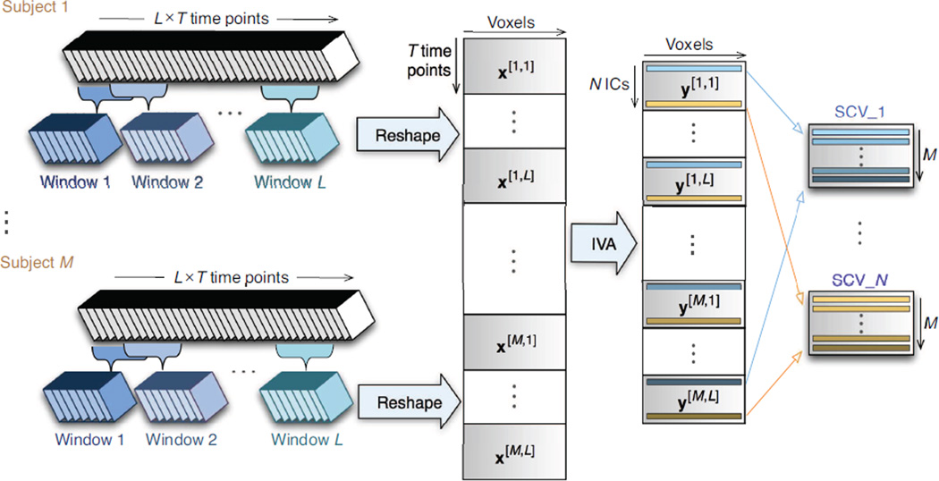
A sliding-window approach is used to segment resting state data. We first divide the original 200 time points for each subject into L = 7 time windows such that each contains T = 50 time points (window size = 75 s) and 50% of time points are overlapping between two sequential windows, as shown in Figure 1. Then the images within each time window are reshaped into a matrix (time points by voxel numbers), denoted by a vector x[m,l],m = 1, …, M, l = 1, …, L if we consider voxels are samples for each time point, where M = 20 is the total number of subjects. Therefore, we perform joint blind source separation on these ML data sets, each of size T × V (where V is the number of voxels).
Figure 1.
Illustration of sliding-window approach to construct data and IVA decomposition to obtain spatial components for dynamic connectivity analysis. ICs: independent components; SCV: source component vector.
2.3. Independent vector analysis
We apply IVA to achieve joint blind source separation and extract spatial components from multiple subjects and different time windows concurrently. We now formulate the IVA problem for the multi-subject, multi-window fMRI analysis. Suppose each data set from the mth subject at the lth window is formed by the linear mixtures of N independent sources,
where is the component vector whose element is the nth underlying component and A is a T-by-N mixing matrix with the nth column representing the time course associated with the nth component. To represent associated components across all subjects, the nth SCV is constructed by taking each nth component from all subjects and windows, i.e., , n = 1, …, N. The goal of IVA is then to find M × L demixing matrices W[m, l] and the corresponding component vector estimates, y[m, l] = W[m, l]x[m, l],m = 1, …, M, l = 1, …, L, such that the estimated SCVs, , n = 1, …, N, are maximally independent from each other, where and is the nth row of W[m, l]. IVA decomposition can be achieved by minimizing the mutual information among SCVs
where ℋ (·) is entropy, is the mutual information within the nth SCV, and C is a constant term that depends only on x[m, l],m = 1, …, M, l = 1, …, L. The term log |detW[m, l]| is due to the change of variables from x[m, l] to y[m, l]. By minimizing this IVA cost function, the dependence among components within each SCV, ℐ(yn), n = 1, …, N, is maximized concurrently.
In this work, we use an IVA implementation, namely IVA-GL, which has been incorporated in group ICA toolbox (GIFT, http://mialab.mrn.org/software). IVA-GL combines two IVA algorithms: IVA-G (Anderson et al., 2012), which exploits only second-order statistical information by multivariate Gaussian assumption and IVA-L (Lee et al., 2008), which utilizes a multivariate Laplace prior for SCV distribution. Thus, the components within each SCV are assumed to be second-order uncorrelated and only higher-order statistics are exploited in IVA-L. To take advantages of both algorithms, we initialize IVA-L with a solution from IVA-G to achieve IVA-GL decomposition. IVA-GL can yield more robust joint blind source separation than using either IVA-L or IVA-G alone (Anderson et al., 2012).
2.4. Functional connectivity measure
After estimating IVA components for the mth subject at the lth window, we quantify sFNC between these components by mutual information (MI). A normalized measure of MI is calculated as (Dionisio et al., 2004)
where and are two estimated spatial components derived from IVA decomposition for the mth subject at the lth window, and ℐ(·,·) is the pairwise MI between them, which we estimate by nonparametric kernel-based method (Peng et al., 2005). λ is in the range of [0, 1) and a value of zero means completely independent. Then the connectivity matrix for the mth subject at the lth time window is constructed using all , 1 ≤ i, ≠ j ≤ N.
2.5. Statistical analysis for connectivity dynamics
To examine connectivity dynamics, we calculate several statistical metrics. At each time window, two-sample t-test is performed to examine significant differences between the HC and SZ groups in the connectivity value between each possible pair of spatial components.
For each subject, we compute the standard deviation (STD) for each connectivity value across all time windows. For the ijth connectivity of the mth subject, the sample STD is
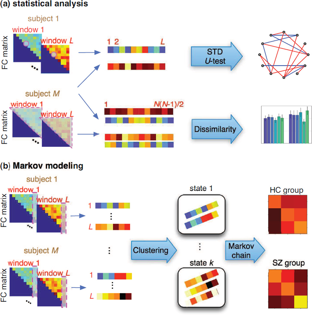
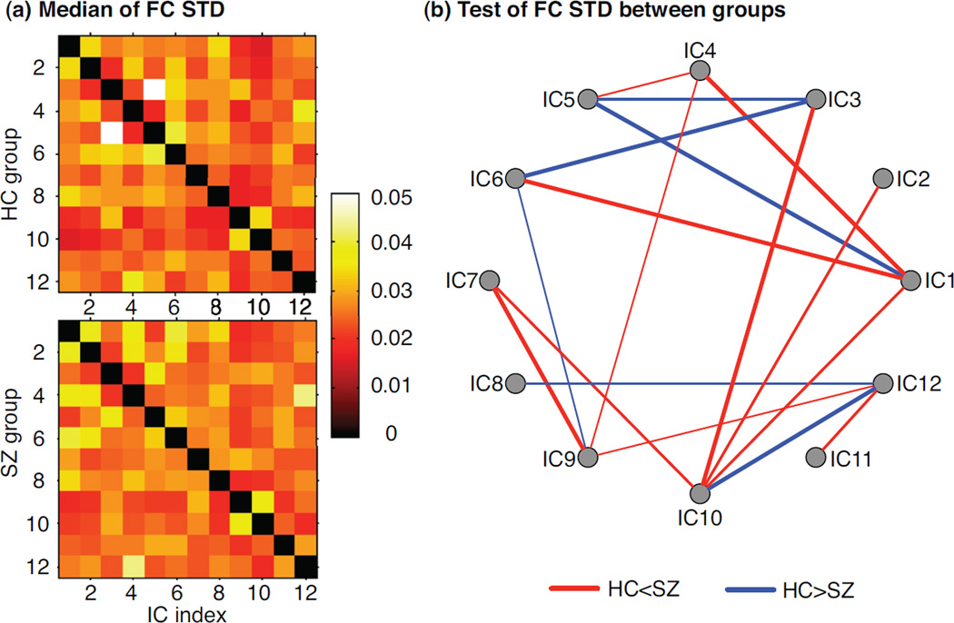
where is the sample mean across time windows. We also calculate the median of STD for all subjects within one population group, as shown in Figure 2(a). These metrics indicate the level of overall dynamics in spatial connectivity between a pair of brain networks. Between different populations, we identify the pairs of brain networks that present significant group differences in sFNC changes by using the Mann-Whitney U-test, a non-parametric hypothesis test for assessing the equality of the population medians of two independent samples (Mann and Whitney, 1947). Therefore, we test the null hypothesis that the HC and SZ groups have equal medians of connectivity STD over time, against the alternative that they do not.
Figure 2.
Flowchart for (a) statistical analysis and (b) Markov modeling analysis for spatial connectivity dynamics.
In addition, we construct a vector containing the connectivity values from all possible pairs of components for each subject and each window. For the mth subject at the lth window, this vector is with total of N(N − 1)/2 entries. For the mth subject, we calculate the Kullback-Leibler divergence (KLD) between this connectivity vectors from different time windows, DKL (q[m, i]||q[m, j])+DKL (q[m, j]||q[m, i]), 1 ≤ i ≠ j ≤ L, in order to quantify the fluctuations in connectivity distribution as a function of time. Similarly, we calculate sample correlation coefficient between connectivity vectors q[m, i] and q[m, j], 1 ≤ i ≠ j ≤ L from different time windows.
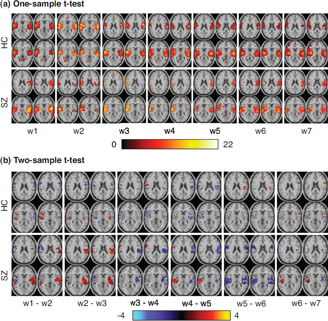
Besides sFNC dynamics, we also study changes in individual components for each group by performing one-sample t-tests across all windows and two-sample t-tests between two sequential windows. A statistical significance level of P < 0.05 is used for both tests and is corrected for false discovery rate (FDR) (Genovese et al., 2002). For each component within one group, MI between subsequent windows, , 1 ≤ i ≤ L − 1, n = 1, …, N, is also calculated to show the temporal variability of activated voxels in the spatial component. Then across time, we compute the STD of , 1 ≤ i ≤ L−1 for the nth component from the mth subject and compare between the HC and SZ groups.
2.6. Markov modeling
We also estimate a first-order Markov chain to examine connectivity dynamics. A clustering approach is adopted to learn the finite states in Markov chain of spatial connectivity. For each component, we have M × L observations, each with N − 1 connectivity values derived between this given component and all other components. We use these connectivity values as features and apply k-means clustering to group these observations into k clusters. Each cluster then represents a state in the Markov chain.
The number of clusters, k, can be determined by cluster validity indices, e.g., the elbow criterion, which is computed as the ratio between within-cluster dissimilarity to between-cluster dissimilarity. However, it yields a relative large cluster number when applied to the data set used in our study. However, we observed that some clusters contain a very small number of observations when using the cluster number determined by the elbow criterion. To avoid such a clustering solution, we use another index, i.e., silhouette (Rousseeuw and Kaufman, 1990), defined as
where for a clustering solution, dW(i) is the average dissimilarity of the ith observation with all other observations within the same cluster, and dB(i) is the lowest average dissimilarity between the ith observation and the observations in other clusters. We use correlation coefficient as the measure of similarity between different observations (thus, dissimilarity is 1−similarity). If c(i) is close to one, this observation is appropriately clustered; if c(i) is close to negative one, this observation might be assigned to a wrong cluster. We explore clustering solutions with different cluster numbers over a range (2 to 15 in our study) to find the number yielding the highest average silhouette.
After obtaining state labels for individual subjects at each time window, we estimate the transition matrix (TM) for each group by counting the state changes between two sequential time windows and using all subjects in each group. The procedure is shown in Figure 2(b).
2.7. Validation of results
For each pair of spatial components, we use a resampling technique (Jafri et al., 2008) to determine whether the average connectivity in the HC group is significantly different from that in the SZ group. We randomly relabel 4 of 10 patients with schizophrenia and 4 of 10 healthy controls. We re-compute the average MI difference between the two shuffled groups in order to build a null distribution. We then calculate a two-sample t-test to determine whether the result is significantly different from the average connectivity difference between the two actual groups.
In addition, we validate the results for sFNC dynamics by repeating the experiment on subsets of subjects to determine whether the same type of dynamic connectivity is presented. The analysis methods, including statistical analysis and Markov modeling analysis, are repeated 20 times. In each of the 20 trials, a number of patients and controls are randomly selected from the full set of subjects. In our experiment, 8 of 10 patients and 8 of 10 controls are chosen each time. For MI test and KLD in statistical analysis, the average value of 20 trials is obtained. For Markov modeling analysis, the occurrence of significant state transfer probability (≥ 0.3) in 20 trials is calculated.
3. Experimental results
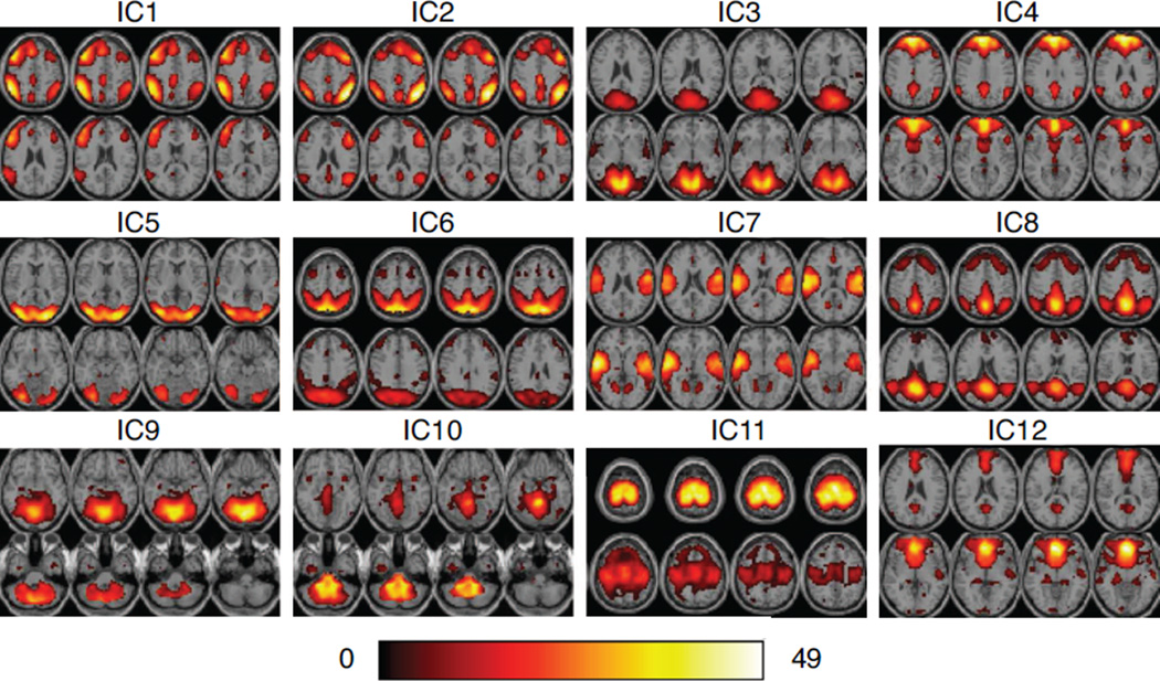
We apply our dynamic connectivity analysis method to the resting state fMRI data set and divide the 200 time points for each subject into 7 windows. Subject-level PCA is performed on individual subject data sets (total of 20 for two groups) to reduce data dimension from 50 to 30. IVA is run on the ensemble of 140 data sets. Since in real applications, both finite data sample size and non-unique decomposition solutions derived from the local optimal points of cost function will induce uncertainty into IVA estimation. Therefore, we perform IVA-GL algorithm 5 times with different initializations and evaluate the stability of IVA decompositions using ICASSO (Himberg et al., 2004), in which the obtained components from all runs are grouped into clusters based on the spatial correlation between them and a quality index for each cluster is calculated based on average inner- and inter- cluster similarities. For the following analysis, we use the estimated components from the most stable run, which is determined using the stability index introduced in our previous work (Ma et al., 2011a). After obtaining 30 reliable component estimates, we visually inspect the spatial maps and remove those components related to artifacts. Finally, total of 12 components of interest for each subject and each window are selected. One-sample t-maps, obtained using all subjects and all windows, of these 12 components are shown in Figure 3. We also note that the IVA-GL algorithm is computationally demanding, e.g., for our parameters and set-up, one run of IVA-GL algorithm requires more than 16 hours on an iMac with 3.5GHz Quad-core Intel Core i7 processor.
Figure 3.
One-sample t-maps for 12 components of interest derived from IVA decomposition, thresholded at P < 0.05 (corrected for multiple comparisons using false discovery rate). Test is performed across all subjects and time windows. Eight slices from each component are shown in the figure.
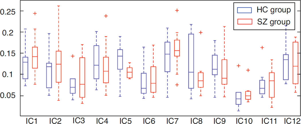
3.1. Changes in individual components
For each spatial component, we calculate MI values between two sequential windows and the STD of MI for each subject. The box plot of STD for two groups is shown in Figure 4. We find that some components exhibit greater temporal variability in spatial maps than others, e.g., IC5 in the HC group and IC7 for the SZ group. At each time window, we perform one-sample t-test for each component. Within a group, we also calculate two-sample t-test for each component between different time windows. One example to demonstrate the significant differences in individual spatial components at different time windows is IC7. As shown in Figure 5, this temporal lobe component from the SZ group varies significantly over time, not only the number and location of activated voxels but also the voxel values; while in the HC group, the voxels within superior temporal regions activate more consistently across time windows, although with variability in voxel values. Consequently, such changes in individual ICs may result in dynamic changes in sFNC.
Figure 4.
Box plot for standard deviation (over 6 time window differences) of mutual information between two sequential time windows for each component. For each box, central line is the median value, the edges represent the 25th and 75th percentiles, the whisker extends to the most extreme non-outlier value, and outliers are shown by “+”
Figure 5.
Changes in spatial maps of IC7 across time windows: (a) one-sample t-test for 10 healthy controls (upper) and 10 patients with schizophrenia (bottom) at each time window, to summarize group trend for each group (P < 0.05, corrected by FDR); (b) two-sample t-test between two sequential windows for healthy group (upper) and patient group (bottom) respectively (window i − window i+1, i = 1,. …, 6, and thresholded at P < 0.05, corrected).
3.2. Statistical analysis for dynamic connectivity
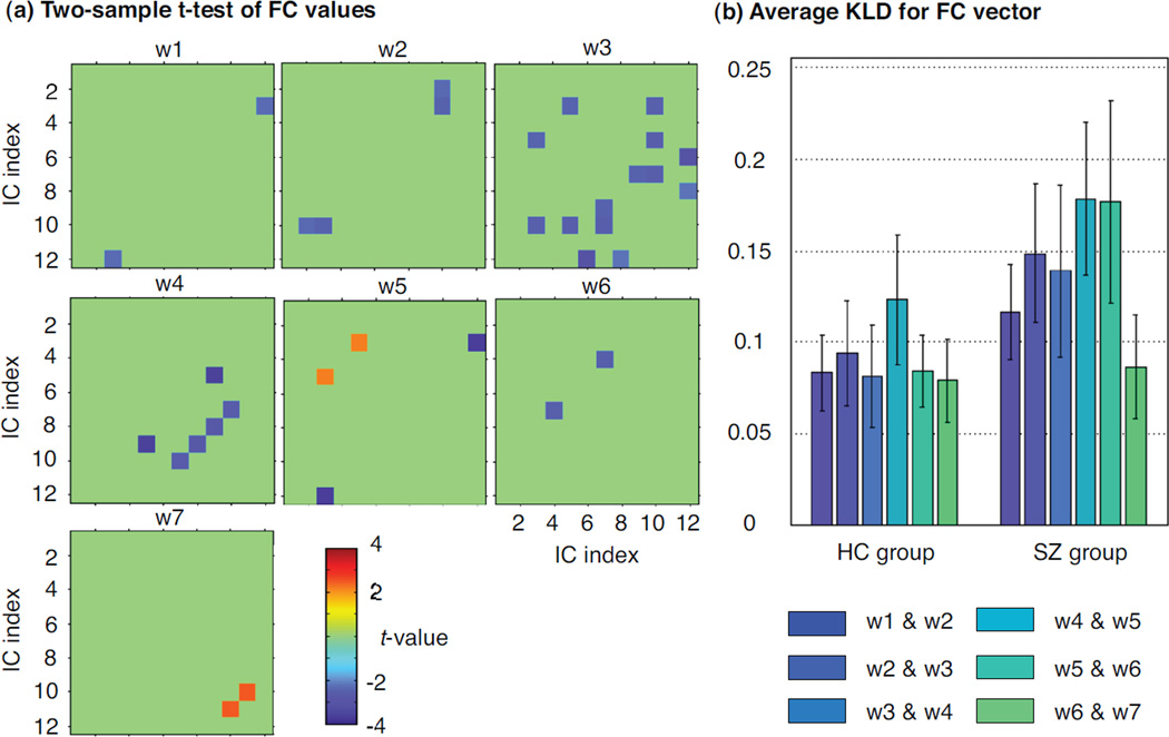
At each time window, we first perform two-sample t-test between two groups for each connectivity. We show the significant group differences in Figure 6(a) if the occurrence percentage of significance is greater than 0.7 in 20 trials of random subject selection. We also perform resampling for validation. All the group differences shown in Figure 6. (a) are significantly different from the shuffled data. Across all time windows, we find that the SZ group has a higher number of connections presenting significantly higher connectivity values than the HC group. The group difference is also indicated by the average KLD of connectivity vectors between two sequential time windows (Figure 6(b)). We find that the SZ group presents larger distance value than the HC group. We obtain similar trend for correlation coefficients between connectivity vectors, but differences between HC and SZ groups decreases.
Figure 6.
(a) Group comparison through a two-sample t-test on the connectivity values of the HC and SZ groups (P < 0.05; positive: HC > SZ; negative: HC < SZ). The significant t-values shown in the figure occur at least 14 out of 20 trials of random subject selection. (b) Average Kullback-Leibler divergence of connectivity vectors between sequential time windows across subjects within each group. Each vector at one time window for one subject contains 66 connectivity values between all possible pairs of 12 components.
For each subject, we also compute the STD for each connectivity over 7 time windows and the median of STD for all subjects within each group, as shown in Figure 7(a). Between different population groups, we perform the Mann-Whitney U-test to identify the pairs of components presenting significant group differences in connectivity STD values, as shown in Figure 7(b). As we observe in individual components, some pairs of components exhibit greater variability in connectivity than others and different pairs of components present significant connectivity dynamics for different groups. For example, the connectivity values between default mode network (DMN) and the orbitofrontal component (IC8 and IC12), and between two visual components (IC3 and IC5), change significantly across time in the HC group; while IC12 and IC9 (cerebellum), or IC7 (temporal lobe) and two cerebellum components (IC9 and IC10) in the SZ group show significant connectivity fluctuations when compared to those in the HC group.
Figure 7.
Statistical metrics to quantify connectivity dynamics: (a) the median of STD for each connection over 7 time windows within each group; (b) Mann-Whitney U-test of each connectivity STD between the HC and SZ groups (P < 0.1). The thicker the line, the more significant is the median value of connectivity changes over time.
3.3. Markov modeling of dynamic connectivity
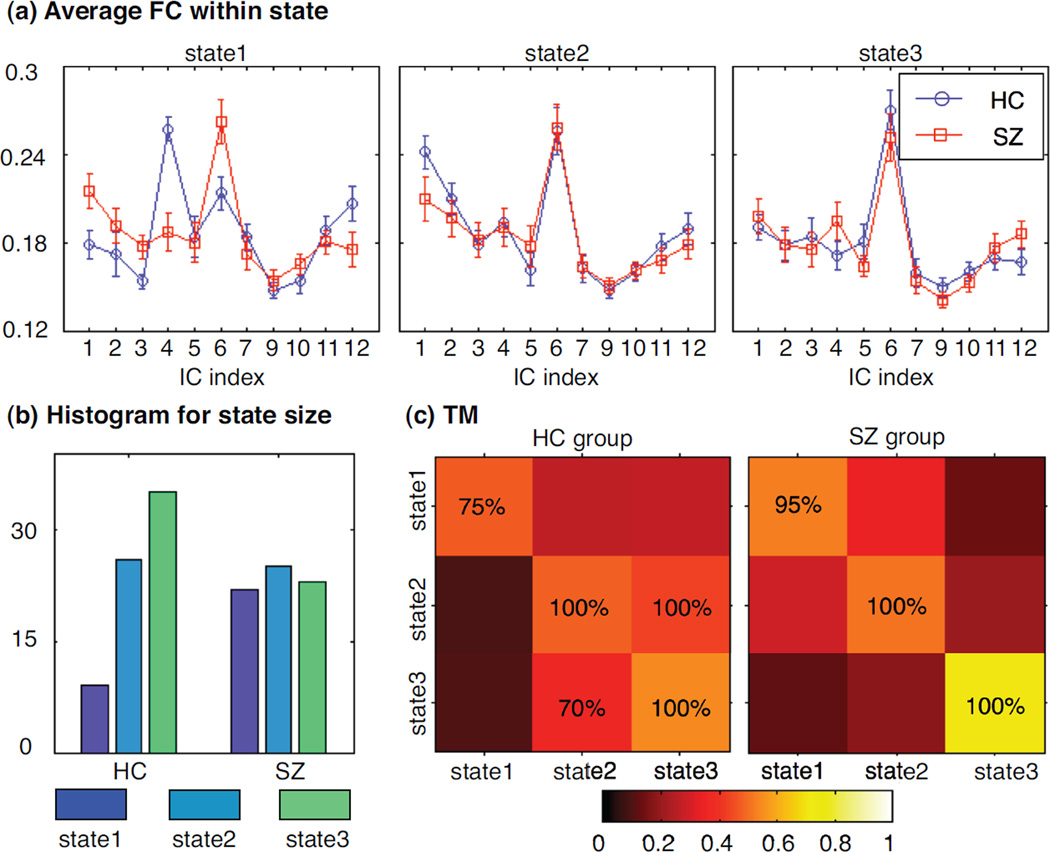
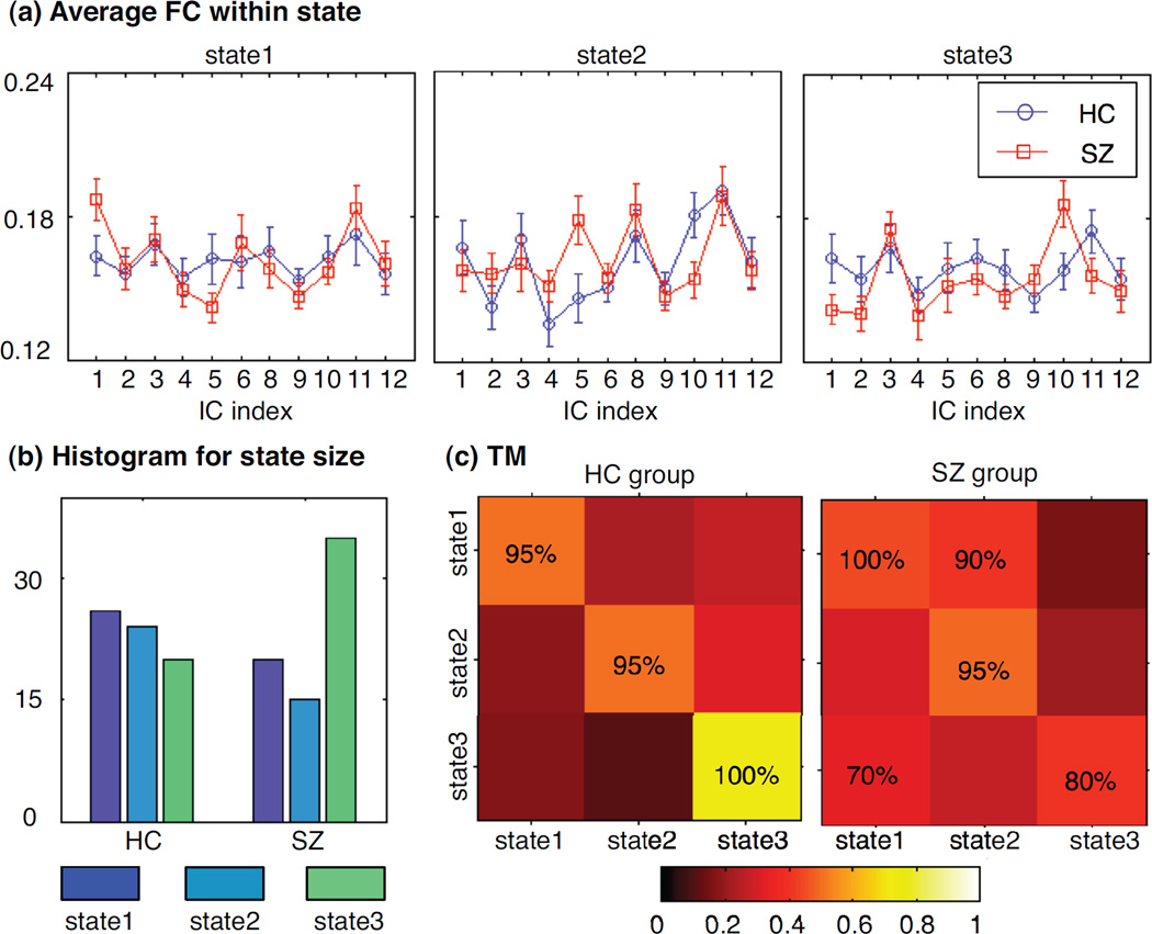
In Markov modeling analysis, we perform k-means clustering for each component to obtain finite states and use the connectivity values between this component and other components as features. Based on average silhouette, we explore the clustering solutions with different numbers of clusters by changing the number from 2 to 15. In our study, the final cluster number is determined as 3 to yield a relative high silhouette and an appropriate histogram of sample number within each cluster. We label each subject at each window by one state (its associated cluster) and then estimate a transition matrix for each group. The Markov modeling results for DMN component are shown in Figure 8. During resting state, DMN component in the HC group has a higher chance to change states; while in the SZ group, DMN component consistently prefers to stay in one state in 20 trials of random subject selection. The average MI within each state and the transition matrix for another component of interest, IC7, are shown in Figure 9. Unlike the DMN component, this temporal lobe component in the SZ group demonstrates more state changes and these state changes are associated with dynamics in the connectivity related to this network. The Markov modeling results further confirm the observations from Figure 7 that different pairs of components in two groups present significant fluctuations in spatial connectivity.
Figure 8.
One example for Markov modeling results: the connectivity between DMN component and all other 11 components, which shows more significant spatial changes over time in healthy control group: (a) average connectivity values within each state for two groups; (b) histogram for each state; (c) the transition matrix for each group, where color represents the transition probability value and the percentage value is the occurrence of significant transition probability in 20 trials of random subject selection. The number of states is determined by silhouette; for the connectivity between DMN and other components, 3 states give the best clustering solution.
Figure 9.
Another Example of Markov modeling results for connectivity between IC7 and other 11 components, which shows more significant spatial changes over time in SZ group. The color in the transition matrix represents the transition probability value and the percentage value is the occurrence of significant transition probability in 20 trials of random subject selection. For the connectivity between temporal lobe component (IC7) and other components, 3 states give the best clustering solution by using silhouette. As shown in Figure 5, this temporal lobe component in the SZ group presents significant changes in spatial maps over time, resulting in connectivity dynamics.
4. Discussion
In this paper, we examine dynamic connectivity changes among pairs of spatial components estimated from fMRI resting state data. Mutual information between components derived from IVA decomposition is used as the measure of spatial functional network connectivity in order to take higher-order statistics into account, instead of second-order correlation or coherence. Using sliding-window approach, statistical and Markov modeling analysis, we compare group variability in spatial connectivity between healthy controls and patients with schizophrenia. With real data, we note that the IVA estimates tend to be not as stable as group ICA results. This is due to the fact that the group ICA approaches involve a group-level PCA, which attempts to find a common signal space for all subjects where to perform the single ICA step and thus introduce an averaging effect over group. However, we perform a subject-level PCA to help with the robustness of the estimation results, although this step is not necessary. In our study, we evaluate the stability of IVA decompositions using ICASSO (Himberg et al., 2004) and use the results from the most stable run.
Using t-tests for individual components over time, we find that during resting state, some components of interest show more spatial fluctuations than others. More importantly, some components in the HC and SZ groups vary differently, e.g., the component including superior and middle temporal regions, which has shown significant group differences in several resting state fMRI studies (Calhoun et al., 2007; Sui et al., 2009). The change in individual components is supporting evidence of connectivity dynamics among these components. Indeed, we observe that some pairs of brain networks yield higher variability in connectivity across time windows than other pairs, and different pairs of brain networks present different connectivity dynamics in different groups. In the HC group, DMN-orbitofrontal, superior visual-inferior visual, parietal-visual, and cerebellum-orbitofrontal connections exhibit significant temporal fluctuations. The DMN-orbitofrontal dynamic connectivity in the HC group has also been found in an ICA-based study using temporal correlation and an AOD task fMRI data set (Sakoğlu et al., 2010). While for the SZ group, left frontal parietal (LFP)-median frontal, temporal-cerebellum, LFP-parietal, and cerebellum-LFP connections present significant fluctuations over time, which may imply weak connections among these regions and disease-related modulations in schizophrenia. In summary, the significant spatial changes in network connectivity in the SZ group mainly occur between frontoparietal, cerebellum and temporal regions. Dysconnectivity or abnormal connectivity has typically been hypothesized as the major pathophysiological mechanism of various mental disorders, especially schizophrenia (Bullmore et al., 1997; Stephan et al., 2009). A number of fMRI studies have studied the dysfunctional temporal, parietal and cerebellum regions and the associated functional connectivity, indicating that these brain networks may play vital roles in the pathophysiology of schizophrenia and other mental diseases (Meyer-Lindenberg et al., 2001; Jafri et al., 2008; Yu et al., 2011; Jones et al., 2012). For example, a resting state connectivity analysis found that most of the disrupted connections in the SZ group were related to the cerebellum and temporal lobe (Liang et al., 2006). Hence, our experimental results provide further support for these previous findings, suggesting focus on the activities of these brain networks and connectivity within/among them.
Through Markov modeling analysis, we confirm our observations from the statistical analysis. For example, the DMN component in the HC group presents a higher probability to transit among three states; while for the SZ group, the DMN component tends to be assigned to single states. For DMN connectivity, the third state seems to be a common state for both groups. While for the HC group, IC4 (anterior DMN) and DMN component present strong association in the first state. This association has been reported in several previous studies of resting-state functional connectivity in DMN (Greicius et al., 2003; Uddin et al., 2009). In the second state, the HC group shows high connectivity values between the frontal parietal components (IC1 and IC2) and DMN, indicating the relationship between the attention network and DMN. These trends are not strong in the SZ group. For temporal lobe connectivity, we find that the SZ group presents a higher probability to transit between states, consistent with the result of our statistical analysis that the temporal lobe component in the SZ group exhibits significantly varying connectivity when compared to the HC group. For the HC group, these three states of temporal lobe connectivity present a level of similarity, such as the relatively high connectivity values with IC3 and IC11. While for the SZ group, strong network coupling varies in different states. Similar trends also can be found in the Markov Modeling results of other networks’ connectivity, such as IC6 (parietal lobe) and IC10 (cerebellum regions).
In addition, we find that the SZ group presents more connectivity dynamics, indicated by the higher KLD value between connectivity vectors over time and more connections showing significantly high STD across time windows. This may provide complementary results to the previous findings that the diversity of static connectivity in the SZ group was increased on average over all brain regions (Bassett et al., 2011; Lynall et al., 2010). In addition, this result may provide support to our previous findings by using clustering and graph-theoretical analysis for spatial connectivity in the HC and SZ groups that patients with schizophrenia presented a tendency to involve more brain regions to perform a cognitive task, possibly as a means of functional compensation, to approach a disorganized, random structure (Ma et al., 2011b).
Other methods such as Bayesian method (Bhattacharya et al., 2006), dynamic causal modeling (Friston et al., 2003), or structural equation modeling (Büchel and Friston, 1997) can be used for dynamic connectivity analysis. However, these methods are all model-based and therefore are limited by the model complexity. They require assumptions for the model parameters and need to estimate these parameters, e.g., certain interaction parameters describing the relation among voxels or networks. On the contrary, the dynamic connectivity method developed here is data-driven and does not require those assumptions or prior knowledge for the temporal domain.
Several limitations pertaining to the methodology used in this paper suggest future work. First, we use mutual information between spatial components as the measure of connectivity. In our previous study (Ma et al., 2011a), we also perform connectivity analysis using temporal correlation between time courses and find similar results but with a certain level of difference. For example, the connectivity between artifact-related components we found by using spatial dependence is not retained when using temporal correlation. Therefore, combining these two measures of connectivity is desirable and may provide a comprehensive measurement of functional activity in the whole brain. One possible way is through back-reconstruction using components and time courses derived from IVA decomposition to obtain the time series for individual brain networks. Second, we examine spatial connectivity changes using a sliding-window approach with window size of 75 s. This window size is in the range of various window sizes used in several previous studies for dynamic connectivity analysis. For example, Sakoğlu et al. verified window size of 96 s (TR = 1.5 s) through a theoretical assessment and simulation study (Sakoğlu et al., 2010); Kiviniemi et al. used a window size of 60 time points (TR = 1.2 s, thus window size = 72 s) for an ICA-based dynamic connectivity study on individual subject level (Kiviniemi et al., 2011); in (Allen et al., 2012), dynamic connectivity is compared between different window sizes and a shorter window size of 44 s is found to provide ability to resolve dynamics, in agreement with the finding that variability in connectivity is reduced when assessed with longer time windows (> 60 s). In our future work, we intend to study connectivity dynamics using a wide range of window sizes (and with continuous windows as opposed to the few snapshots). Another issue in this study is that we only utilize a relatively small number of time windows due to the demanding running time of IVA-GL algorithm. Therefore, future work also includes developing more efficient ways to obtain and analyze a large number of highly overlapping windows, which may allow dynamic connectivity analysis in the frequency domain. To this end, we can employ a more effective IVA implementation using the decoupling method (Li and Zhang, 2007; Li and Adalı, 2010). IVA with Kotz type distribution prior (Anderson et al., 2013) is another option to achieve efficient and effective joint blind source separation. Furthermore, we will investigate the relationship between connectivity dynamics during resting state and features of patients with schizophrenia, for example, age and PANSS scores; we will examine task-induced connectivity fluctuations and include more subjects in our future work.
Supplementary Material
RESEARCH HIGHLIGHTS.
Dynamic changes of spatial connectivity among brain networks are examined
Higher-order dependence between spatial component pairs is taken into account
IVA is applied to extract time varying components and capture group variability
Statistical and Markov modeling analyses are proposed to quantify dynamic changes
Patients with schizophrenia show less stable patterns of spatial concordance
Acknowledgments
This work is supported by the NSF grants NSF-IIS 1017718 and NSF-CCF 1117056. We thank the research staff at the University of New Mexico and the Mind Research Network who collected, processed and shared the data. We appreciate the valuable advice given by the members of Machine Learning for Signal Processing Laboratory in University of Maryland, Baltimore County.
Footnotes
Publisher's Disclaimer: This is a PDF file of an unedited manuscript that has been accepted for publication. As a service to our customers we are providing this early version of the manuscript. The manuscript will undergo copyediting, typesetting, and review of the resulting proof before it is published in its final citable form. Please note that during the production process errors may be discovered which could affect the content, and all legal disclaimers that apply to the journal pertain.
References
- Allen EA, Damaraju E, Plis SM, Erhardt EB, Eichele T, Calhoun VD. Tracking whole-brain connectivity dynamics in the resting state. Cerebral Cortex. 2012 doi: 10.1093/cercor/bhs352. [DOI] [PMC free article] [PubMed] [Google Scholar]
- Allen EA, Erhardt EB, Damaraju E, Gruner W, Segall JM, Silva RF, Havlicek M, Rachakonda S, Fries J, Kalyanam R. A baseline for the multivariate comparison of resting-state networks. Frontiers in Systems Neuroscience. 2011a;5:2. doi: 10.3389/fnsys.2011.00002. [DOI] [PMC free article] [PubMed] [Google Scholar]
- Allen EA, Erhardt EB, Wei Y, Eichele T, Calhoun VD. Capturing inter-subject variability with group independent component analysis of fMRI data: a simulation study. Neuroimage. 2011b;59(4):4141–4159. doi: 10.1016/j.neuroimage.2011.10.010. [DOI] [PMC free article] [PubMed] [Google Scholar]
- Anderson M, Adalı T, Li X-L. Joint blind source separation with multivariate Gaussian model: algorithms and performance analysis. IEEE Transactions on Signal Processing. 2012;60(4):1672–1683. [Google Scholar]
- Anderson M, Fu G-S, Phlypo R, Adalı T. Independent vector analysis, the Kotz distribution, and performance bounds; Proceedings of IEEE International Conference on Acoustics Speech and Signal Processing (ICASSP’13); 2013. [Google Scholar]
- Baldassano C, Iordan MC, Beck DM, Fei-Fei L. Voxel-level functional connectivity using spatial regularization. Neuroimage. 2012;63(3):1099–1106. doi: 10.1016/j.neuroimage.2012.07.046. [DOI] [PMC free article] [PubMed] [Google Scholar]
- Bassett DS, Nelson BG, Mueller BA, Camchong J, Lim KO. Altered resting state complexity in schizophrenia. Neuroimage. 2011;59:2196–2207. doi: 10.1016/j.neuroimage.2011.10.002. [DOI] [PMC free article] [PubMed] [Google Scholar]
- Bhattacharya S, Ringo Ho MH, Purkayastha S. A Bayesian approach to modeling dynamic effective connectivity with fMRI data. Neuroimage. 2006;30(3):794–812. doi: 10.1016/j.neuroimage.2005.10.019. [DOI] [PubMed] [Google Scholar]
- Biswal B, Zerrin Yetkin F, Haughton VM, Hyde JS. Functional connectivity in the motor cortex of resting human brain using echo-planarMRI. Magnetic Resonance in Medicine. 1995;34(4):537–541. doi: 10.1002/mrm.1910340409. [DOI] [PubMed] [Google Scholar]
- Büuchel C, Friston KJ. Modulation of connectivity in visual pathways by attention: cortical interactions evaluated with structural equation modeling and fMRI. Cerebral Cortex. 1997;7(8):768–778. doi: 10.1093/cercor/7.8.768. [DOI] [PubMed] [Google Scholar]
- Bullmore ET, Frangou S, Murray RM. The dysplastic net hypothesis: an integration of developmental and dysconnectivity theories of schizophrenia. Schizophrenia Research. 1997;28(2):143–156. doi: 10.1016/s0920-9964(97)00114-x. [DOI] [PubMed] [Google Scholar]
- Calhoun V, Adali T, Pearlson G, Pekar J. Spatial and temporal independent component analysis of functional MRI data containing a pair of task-related waveforms. Human brain mapping. 2001a;13(1):43–53. doi: 10.1002/hbm.1024. [DOI] [PMC free article] [PubMed] [Google Scholar]
- Calhoun VD, Adalı T. Multi-subject independent component analysis of fMRI: A decade of intrinsic networks, default mode, and neurodiagnostic discovery. IEEE Reviews in Biomedical Engineering. 2012;5:60–73. doi: 10.1109/RBME.2012.2211076. [DOI] [PMC free article] [PubMed] [Google Scholar]
- Calhoun VD, Adalı T, Pearlson GD, Pekar JJ. A method for making group inferences from functional MRI data using independent component analysis. Human Brain Mapping. 2001b;14(3):140–151. doi: 10.1002/hbm.1048. [DOI] [PMC free article] [PubMed] [Google Scholar]
- Calhoun VD, Kiehl KA, Pearlson GD. Modulation of temporally coherent brain networks estimated using ICA at rest and during cognitive tasks. Human Brain Mapping. 2008;29(7):828–838. doi: 10.1002/hbm.20581. [DOI] [PMC free article] [PubMed] [Google Scholar]
- Calhoun VD, Maciejewski PK, Pearlson GD, Kiehl KA. Temporal lobe and “default” hemodynamic brain modes discriminate between schizophrenia and bipolar disorder. Human Brain Mapping. 2007;29(11):1265–1275. doi: 10.1002/hbm.20463. [DOI] [PMC free article] [PubMed] [Google Scholar]
- Chang C, Glover GH. Time-frequency dynamics of resting-state brain connectivity measured with fMRI. Neuroimage. 2010;50(1):81–98. doi: 10.1016/j.neuroimage.2009.12.011. [DOI] [PMC free article] [PubMed] [Google Scholar]
- Danielyan A, Nasrallah HA. Neurological Disorders in Schizophrenia. Psychiatric Clinics of North America. 2009;32(4):719–757. doi: 10.1016/j.psc.2009.08.004. [DOI] [PubMed] [Google Scholar]
- Dea JT, Anderson M, Allen EA, Calhoun VD, Adalı T. IVA for multi-subject fMRI analysis: a comparative study using a new simulation toolbox. Proceedings of IEEE International Workshop on Machine Learning for Signal Processing. 2011 [Google Scholar]
- Dionisio A, Menezes R, Mendes DA. Mutual information: ameasure of dependency for nonlinear time series. Physica A: Statistical Mechanics and its Applications. 2004;344(1):326–329. [Google Scholar]
- Esposito F, Scarabino T, Hyvärinen A, Himberg J, Formisano E, Comani S, Tedeschi G, Goebel R, Seifritz E, Di Salle F. Independent component analysis of fMRI group studies by self-organizing clustering. Neuroimage. 2005;25(1):193–205. doi: 10.1016/j.neuroimage.2004.10.042. [DOI] [PubMed] [Google Scholar]
- Freire L, Roche A, Mangin JF. What is the best similarity measure for motion correction in fMRI time series? IEEE Transactions on Medical Imaging. 2002;21(5):470–484. doi: 10.1109/TMI.2002.1009383. [DOI] [PubMed] [Google Scholar]
- Friston KJ, Harrison L, Penny W. Dynamic causal modelling. Neuroimage. 2003;19(4):1273–1302. doi: 10.1016/s1053-8119(03)00202-7. [DOI] [PubMed] [Google Scholar]
- Genovese CR, Lazar NA, Nichols T. Thresholding of statistical maps in functional neuroimaging using the false discovery rate. Neuroimage. 2002;15(4):870–878. doi: 10.1006/nimg.2001.1037. [DOI] [PubMed] [Google Scholar]
- Greicius MD, Krasnow B, Reiss AL, Menon V. Functional connectivity in the resting brain: a network analysis of the default mode hypothesis. Proceedings of the National Academy of Sciences. 2003;100(1):253–258. doi: 10.1073/pnas.0135058100. [DOI] [PMC free article] [PubMed] [Google Scholar]
- Himberg J, Hyvärinen A, Esposito F. Validating the independent components of neuroimaging time series via clustering and visualization. Neuroimage. 2004;22(3):1214–1222. doi: 10.1016/j.neuroimage.2004.03.027. [DOI] [PubMed] [Google Scholar]
- Hutchison RM, Womelsdorf T, Allen EA, Bandettini PA, Calhoun VD, Corbetta M, Penna SD, Duyn J, Glover G, Gonzalez-Castillo J, et al. Dynamic functional connectivity: Promises, issues, and interpretations. NeuroImage. 2013;80:360–378. doi: 10.1016/j.neuroimage.2013.05.079. [DOI] [PMC free article] [PubMed] [Google Scholar]
- Hutchison RM, Womelsdorf T, Gati JS, Everling S, Menon RS. Resting-state networks show dynamic functional connectivity in awake humans and anesthetized macaques. Human brain mapping. 2012;34(9):2154–2177. doi: 10.1002/hbm.22058. [DOI] [PMC free article] [PubMed] [Google Scholar]
- Iritani S. Neuropathology of schizophrenia: A mini review. Neuropathology. 2007;27(6):604–608. doi: 10.1111/j.1440-1789.2007.00798.x. [DOI] [PubMed] [Google Scholar]
- Jafri MJ, Pearlson GD, Stevens M, Calhoun VD. A method for functional network connectivity among spatially independent resting-state components in schizophrenia. NeuroImage. 2008;39(4):1666–1681. doi: 10.1016/j.neuroimage.2007.11.001. [DOI] [PMC free article] [PubMed] [Google Scholar]
- Jones DT, Vemuri P, Murphy MC, Gunter JL, Senjem ML, Machulda MM, Przybelski SA, Gregg BE, Kantarci K, Knopman DS, Boeve BF, Petersen RC, Jack CR., Jr Nonstationarity in the “resting brain’s” modular architecture. PloS one. 2012;7:e39731. doi: 10.1371/journal.pone.0039731. [DOI] [PMC free article] [PubMed] [Google Scholar]
- Kang J, Wang L, Yan C, Wang J, Liang X, He Y. Characterizing dynamic functional connectivity in the resting brain using variable parameter regression and Kalman filtering approaches. Neuroimage. 2011;56(3):1222–1234. doi: 10.1016/j.neuroimage.2011.03.033. [DOI] [PubMed] [Google Scholar]
- Kiviniemi V, Vire T, Remes J, Elseoud AA, Starck T, Tervonen O, Nikkinen J. A sliding time-window ICA reveals spatial variability of the default mode network in time. Brain Connectivity. 2011;1(4):339–347. doi: 10.1089/brain.2011.0036. [DOI] [PubMed] [Google Scholar]
- Lee JH, Lee TW, Jolesz FA, Yoo SS. Independent vector analysis (IVA): multivariate approach for fMRI group study. Neuroimage. 2008;40(1):86–109. doi: 10.1016/j.neuroimage.2007.11.019. [DOI] [PubMed] [Google Scholar]
- Li X-L, Adalı T. Independent component analysis by entropy bound minimization. IEEE Transactions on Signal Processing. 2010;58(10):5151–5164. [Google Scholar]
- Li X-L, Zhang X-D. Nonorthogonal joint diagonalization free of degenerate solution. IEEE Transactions on Signal Processing. 2007;55(5):1803–1814. [Google Scholar]
- Liang M, Zhou Y, Jiang T, Liu Z, Tian L, Liu H, Hao Y. Widespread functional disconnectivity in schizophrenia with resting-state functional magnetic resonance imaging. Neuroreport. 2006;17(2):209–213. doi: 10.1097/01.wnr.0000198434.06518.b8. [DOI] [PubMed] [Google Scholar]
- Lynall ME, Bassett DS, Kerwin R, McKenna PJ, Kitzbichler M, Muller U, Bullmore E. Functional connectivity and brain networks in schizophrenia. The Journal of Neuroscience. 2010;30(28):9477–9487. doi: 10.1523/JNEUROSCI.0333-10.2010. [DOI] [PMC free article] [PubMed] [Google Scholar]
- Ma S, Correa NM, Li X-L, Eichele T, Calhoun VD, Adalı T. Automatic identification of functional clusters in fMRI data using spatial dependence. IEEE Transactions on Biomedical Engineering. 2011a;58(12):3406–3417. doi: 10.1109/TBME.2011.2167149. [DOI] [PMC free article] [PubMed] [Google Scholar]
- Ma S, Eichele T, Correa NM, Calhoun VD, Adalı T. Hierarchical and graphical analysis of fMRI network connectivity in healthy and schizophrenic groups. Proceedings of IEEE International Symposium on Biomedical Imaging (ISBI’11) 2011b [Google Scholar]
- Ma S, Phlypo R, Calhoun VD, Adalı T. Capturing group variability using IVA: a simulation study and graph-theoretical analysis; Proceedings of IEEE International Conference on Acoustics Speech and Signal Processing (ICASSP’13); 2013. [Google Scholar]
- Mann HB, Whitney DR. On a test of whether one of two random variables is stochastically larger than the other. The annals of mathematical statistics. 1947;18(1):50–60. [Google Scholar]
- McKeown MJ, Makeig S, Brown GG, Jung TP, Kindermann SS, Bell AJ, Sejnowski TJ. Analysis of fMRI data by blind separation into independent spatial components. Human Brain Mapping. 1998;6:160–188. doi: 10.1002/(SICI)1097-0193(1998)6:3<160::AID-HBM5>3.0.CO;2-1. [DOI] [PMC free article] [PubMed] [Google Scholar]
- Meyer-Lindenberg A, Poline JB, Kohn PD, Holt JL, Egan MF, Weinberger DR, Berman KF. Evidence for abnormal cortical functional connectivity during working memory in schizophrenia. American Journal of Psychiatry. 2001;158(11):1809–1817. doi: 10.1176/appi.ajp.158.11.1809. [DOI] [PubMed] [Google Scholar]
- Michael AM, Miller R, Anderson M, Adalı T, Calhoun VD. Capturing inter-subject variability in fMRI networks: A performance evaluation of ICA and IVA. Seattle, WA: Organization for Human Brain Mapping; 2013. [Google Scholar]
- Peng H, Long F, Ding C. Feature selection based on mutual information criteria of max-dependency, max-relevance, and min-redundancy. IEEE Transactions on Pattern Analysis and Machine Intelligence. 2005;27(8):1226–1238. doi: 10.1109/TPAMI.2005.159. [DOI] [PubMed] [Google Scholar]
- Rousseeuw PJ, Kaufman L. Finding groups in data: an introduction to cluster analysis. John, John Wiley and Sons; 1990. [Google Scholar]
- Sakoğlu Ü, Pearlson GD, Kiehl KA, Wang YM, Michael AM, Calhoun VD. A method for evaluating dynamic functional network connectivity and task-modulation: application to schizophrenia. Magnetic Resonance Materials in Physics, Biology and Medicine. 2010;23(5):351–366. doi: 10.1007/s10334-010-0197-8. [DOI] [PMC free article] [PubMed] [Google Scholar]
- Starck T, Nikkinen J, Remes J, Rahko J, Moilanen I, Tervonen O, Kiviniemi V. Fluctuating connectivity between default mode sub-networks in ASDs. Human Brain Mapping. 2012 [Google Scholar]
- Stephan KE, Friston KJ, Frith CD. Dysconnection in schizophrenia: from abnormal synaptic plasticity to failures of self-monitoring. Schizophr. Bull. 2009;35:509–527. doi: 10.1093/schbul/sbn176. [DOI] [PMC free article] [PubMed] [Google Scholar]
- Sui J, Adalı T, Pearlson GD, Calhoun VD. An ICA-based method for the identification of optimal fMRI features and components using combined group-discriminative techniques. Neuroimage. 2009;46(1):73–86. doi: 10.1016/j.neuroimage.2009.01.026. [DOI] [PMC free article] [PubMed] [Google Scholar]
- Uddin LQ, Clare Kelly AM, Biswal BB, Xavier Castellanos F, Milham MP. Functional connectivity of default mode network components: correlation, anticorrelation, and causality. Human Brain Mapping. 2009;30(2):625–637. doi: 10.1002/hbm.20531. [DOI] [PMC free article] [PubMed] [Google Scholar]
- van Os J, Kapur S. Schizophrenia. Lancet. 2009;374(9690):635–645. doi: 10.1016/S0140-6736(09)60995-8. [DOI] [PubMed] [Google Scholar]
- Yu Q, Sui J, Rachakonda S, He H, Pearlson GD, Calhoun VD. Altered small-world brain networks in temporal lobe in patients with schizophrenia performing an auditory oddball task. Frontiers in Systems Neuroscience. 2011;5:7. doi: 10.3389/fnsys.2011.00007. [DOI] [PMC free article] [PubMed] [Google Scholar]
Associated Data
This section collects any data citations, data availability statements, or supplementary materials included in this article.


