

Abstract
Built environment factors constrain individual level behaviors and choices, and thus are receiving increasing attention to assess their influence on health. Traditional regression methods have been widely used to examine associations between built environment measures and health outcomes, where a fixed, pre-specified spatial scale (e.g., 1 mile buffer) is used to construct environment measures. However, the spatial scale for these associations remains largely unknown and misspecifying it introduces bias. We propose the use of distributed lag models (DLMs) to describe the association between built environment features and health as a function of distance from the locations of interest and circumvent a-priori selection of a spatial scale. Based on simulation studies, we demonstrate that traditional regression models produce associations biased away from the null when there is spatial correlation among the built environment features. Inference based on DLMs is robust under a range of scenarios of the built environment. We use this innovative application of DLMs to examine the association between the availability of convenience stores near California public schools, which may affect children’s dietary choices both through direct access to junk food and exposure to advertisement, and children’s body mass index z-scores (BMIz).
INTRODUCTION
Built environmental factors and community resources may be critically important determinants of disease because they directly constrain individual choices and behaviors.1,2 For example, environment attributes near or around schools, particularly the availability of commercial establishments offering “junk” food, are under scrutiny as possible contributors to the childhood obesity epidemic.3-7 Convenience stores are an example of establishments that sell high energy, low nutrition foods. The availability of convenience stores near schools may increase children’s junk food consumption, directly through purchasing on the way to and from school and indirectly through excess exposure to advertising,8,9 and affect children’s weight status.3,4
The spatial scale used to construct environmental measures is an important consideration in efforts to estimate associations between built environment factors and health.10 A common approach is to construct a buffer (i.e., a circular area) around locations of interest (e.g., schools) and count environment features (e.g., number of convenience stores) within the buffer. Studies that use buffers to measure environment attributes typically choose the buffer’s radius in an ad hoc manner, sometimes justifying the selected radius by distance travel time (e.g., children could walk ½ mile in 5-10 minutes11,12). However, the causally relevant distances within which environment features may affect health remain unknown,10 and empirical methods to determine them are understudied or do not perform well.13,14
Incorrect spatial scale selection when assessing environment-health associations can yield incorrect inferences15,16. For instance, consider data generated from the model Y = α + βX(A5) + ε, where β ≠ 0, X(A5) is an environmental measure constructed within a 5 mile buffer, while ε is a residual error. Not knowing the true buffer size, suppose we instead fit Y = θ0 + θ1X(A3) + ε′. If the environment measure computed from distance 3 to 5 miles from the locations, say X(A3−5), is correlated with X(A3), the estimated θ1 will suffer from omitted variable bias; the bias may be away from the null.
In this paper we (1) describe distributed lag models and show how they can be applied to investigate built environment-health associations; and, as a case study, (2) use distributed lag models to examine the association between the presence of convenience stores near schools and children’s body mass index z-scores (BMIz).
METHODS
Distributed Lag Models
Distributed lag models have a long history in economics;17,18 more recently they have been used in air pollution studies19-25 to examine how health outcomes may be affected by air pollution during prior periods (i.e., ‘lagged’ exposures). For built environment research, we define the lagged exposure as the environment feature between two radii, rl−1 and rl from study locations, l = 1, 2, … , L, where r0 = 0; e.g., the lagged exposure is the number of convenience stores within “ring”-shaped areas around schools.
Let Yi be a continuous outcome measured at location i, Xi(rl−1;rl), l = 1, 2, … , L, be an environment feature measured within a ring-shaped area26 around location i between radii rl−1 and rl.; and rL be the maximum distance around locations beyond which there is no association between the environment feature and the outcome. The distributed lag model is
| (1) |
where εi ~ N(0, τ2), β0 represents the intercept. The association of the environment feature measured between radii rl−1 and rl around the locations and the outcome is β (rl−1; rl); for instance, the difference in children’s BMIz per additional convenience store between radii rl−1 and rl (see Figure 1A). New insights can be gained from the distributed lag model coefficients by examining the magnitude and pattern (shape) of β(rl−1; rl) as a function of distance from locations of interest: we may be able to identify distances at which the built environment factor is strongly associated with the outcome and at which distance the association vanishes. Although indirectly, this allows us to identify the spatial scales for a given outcome-exposure association.
Figure 1.
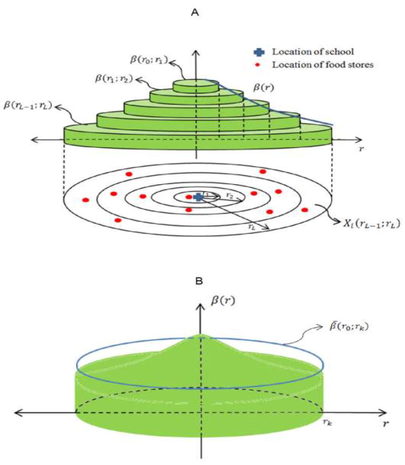
(A) Ring-shaped areas within which built environment features are ascertained and corresponding distributed lag coefficients. (B) Averaged coefficient associated with features within buffer of radius rk, β̄(0; rk); larger radius rk will result in smaller averaged coefficient because effect is averaged over a larger area.
Since the true associations between the outcome and built environment features within ring-shaped areas are likely similar in adjacent rings, we model the coefficients β(rl−1; rl as a smooth function of distance from the locations of interest using smoothing splines22,27 (see eAppendix for implementation details). While various ways for constraining the distributed lag coefficients have been proposed,23,25 we used a smoothing spline approach22 since knot selection is not required and relatively fewer assumptions are imposed. Smoothing splines are an attractive option for modeling the coefficients because: (1) we would not typically expect associations to change abruptly across distance; (2) they alleviate numerical/singularity problems that may arise when many locations have zero food stores between two given radii rl−1 and rl; and (3) they resolve issues regarding the choice of the number of rings because by controlling the degrees of freedom used for estimating the L lag coefficients. The number of lags L<n needs to be large enough to avoid coarser estimates (see simulation section), and can be chosen so that the ring width is small enough for practical purposes (e.g., one street block).
The units of the built environment feature captured by Xi(rl−1; rl) naturally impact the interpretation of β (rl−1; rl). In our application, we used the total number of convenience stores, however, other definitions could be used, such as the density of convenience stores per square mile. For density measures, the distributed lag coefficients can be readily calculated by transforming the parameters in (1): coefficients of the association between the count per unit area and outcome are equal to the coefficients in (1) weighed by the area of the ring, i.e., .
Estimation of distributed lag model parameters can be carried out using either a frequentist or a Bayesian approach in readily available software,28-30 and the smoothing parameter for the coefficients can be selected by representing the smooth function as mixed model or via generalized cross validation. We opted for the latter using a Bayesian approach (see eAppendix for details and sample R code) because this allows us to account for the uncertainty in the penalty parameters and easily derive the variance of estimated coefficients.
Connection between distributed lag models and Traditional Approaches
Traditional linear models, e.g., Yi = θ0 + θ1,rk Xi(0; rk) + εi, are the widespread approach to estimate the average association between built environment measures within a buffer of radius rk [i.e.,Xi(0; rk)] and health outcomes. Implicitly, traditional linear models assume that the outcome-environment association within distance rk is constant and no association beyond distance rk exists (e.g., Figure 3A). Our proposed distributed lag model allows us to relax both of these assumptions by allowing the coefficients to vary smoothly as a function of distance (e.g., Figure 3B). In addition, our model enables us to easily calculate the average buffer effect β̄ (0;rk) up to a given distance rk (e.g., the average difference in children’s BMIz per one additional convenient stores within a buffer of radius rk) by computing the average height of the solid shape depicted in Figure 1B, i.e.,
| (2) |
To see this, first consider the average buffer effect up to distance rk in the density scale. Because the association between distance rl−1 and rl in the density scale is , the sum of the area-weighted associations, , gives the total association within the buffer of radius rk. Division by the total area of the buffer, , yields the average association for the buffer area. In air pollution research, the simple sum of the distributed lag coefficients represents the overall health impact of a unit difference in exposure on the previous k days; in our case the distributed lag coefficients have to be weighted by the area of the rings to obtain an analogous interpretation.
Figure 3.
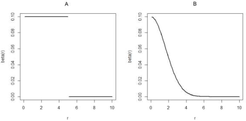
True function β(r) used in simulation studies to represent impact of built environment features as a function of distance, r, from study locations. (A) Step function: β(r) = 0.1 if r ≤ 5, 0 otherwise represents assumption that associations are constant within the a given buffer size (i.e. r ≤ 5), and are zero outside the buffer. (B) Curve: β(r) = 0.1fz (r)/f(0), where fz(r) is a normal density with mean 0 and standard deviation 5/3, represents the assumption that associations decay smoothly towards zero.
Differences in Distributed Lag Coefficients by Subject Characteristics
Distributed lag models can be expanded to allow the association between a health outcome and built environment features to vary by subject characteristics. Associations between features of the built environment and children’s BMIz might be different by age or grade, for instance, if school policies allow or disallow children to leave school during lunch periods depending on a child’s age. To investigate whether the distributed lag effects vary according to subjects characteristics, equation (1) could include interaction terms between Xi(rl−1; rl), l = 1,2, …, L, and a covariate Zi: i.e., θ (rl−1;rl) Xi (rl−1;rl)Zi. Interaction coefficients θ (rl−1; rl) have the usual interpretation, but the magnitude of the interaction can vary over distance from locations of interest.
Extensions of the model
Distributed lag models can be extended in several directions to examine different types of outcomes. Generalized linear distributed lag models can be used if the observed outcome Yi is binary or a count. In our motivating example, although our outcome is approximately normal, the assumption of constant variance, typical of linear models, does not hold. In this situation a weighted distributed lag model may be used, where the error terms εi are modeled as εi ~ N(0, τ2/wi) and wi is a known weight for the ith observation. Fitting a weighted distributed lag model is rather straightforward31: proceeding as in weighted least squares, the outcome Yi and all covariates are transformed as and , l = 1, 2, … , L, (and similarly for any additional predictors), and the distributed lag model in equation (1) is fitted to the transformed data. Interpretation of the regression coefficients remains unchanged. Multilevel models to account for clustering of subjects within larger units can also be implemented (see Data and Methods).
Simulations
We performed a simulation study to assess the distributed lag model’s ability to estimate coefficients as a function of distance, and to compare the traditional linear and distributed lag models in terms of inferences for the associations at pre-specified distances under various degrees of clustering in the built environment. Full details of the simulation settings are in the eAppendix. Briefly, we simulated 1000 datasets by first sampling food store locations from a spatial domain with various degrees of clustering (Figure 2), and sampling school locations at random from the same domain. We generated outcomes from linear model (1) under two assumptions for the true shape of the coefficients β as a function of distance: We used a step function [β(r) =0.1 if r ≤ 5, 0 otherwise] to mimic the assumption made by traditional linear models that effects are zero outside a specified buffer (Figure 3A); and a curve [ β(r) = 0.1 fz(r)/f(0), where fz(r) is a normal density with mean 0 and standard deviation 5/3] represent smoothly decreasing built environment effects with longer distances from locations of interest (Figure 3B). Distributed lag models (using with L = 100 and rL = 10) and traditional linear models using a-priori chosen distances rk = 2.5, 5, and 7.5 were fitted. The same distances were used to calculate average buffer effects β̄(0;rk) from distributed lag models using (2). Different sample sizes and values of model R2 were used.
Figure 2.
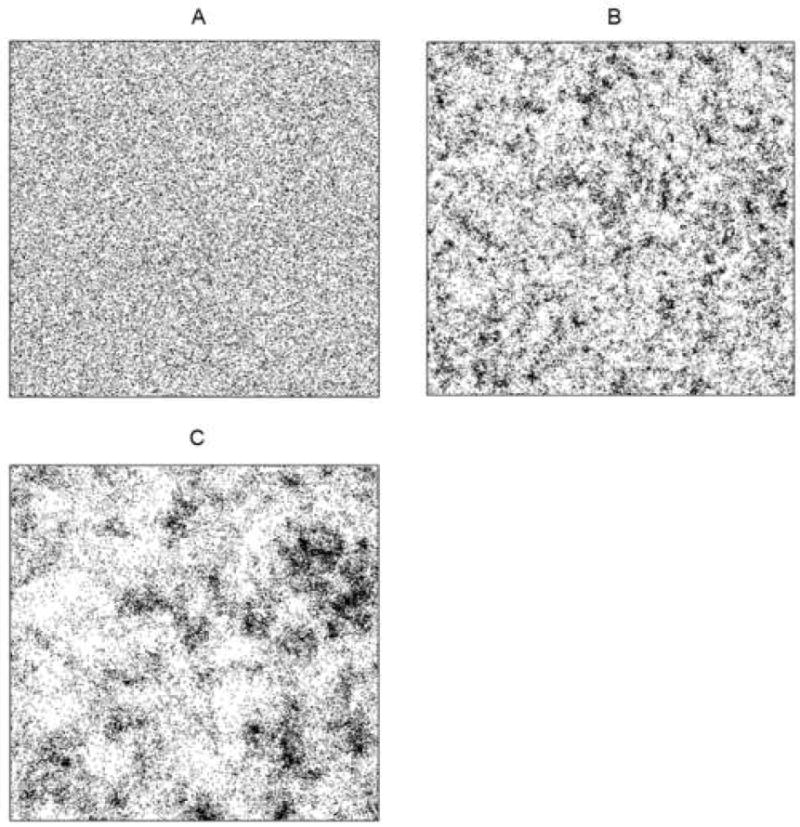
Spatial domains used in the simulation study depicting three assumed clustering settings for built environment features: locations of food stores are sampled from (A) a homogeneous Poisson point process (no clustering) and an inhomogeneous Poisson point process with intensity functions that leads to (B) a small amount of clustering (spatial range =5), (C) a large amount of clustering (spatial range = 20).
Children’s BMIz and Convenience Stores in California: Data and Methods
We used FitnessGram data for 5th and 7th grade children who attended public schools in California in 2009 to examine associations between availability of convenience stores near schools and children’s BMI z-scores (BMIz). FitnessGram data are publicly available from the California Department of Education (CDE) and include measures of children’s weight and height, grade (we used 5th and 7th), age (we categorized as 10, 11, 12, 13, and 14 or more), sex, and race/ethnicity (we used non-Hispanic White and Hispanic only). The analysis included only two of California’s most prevalent race/ethnicity groups because we were interested in illustrating how differences in distributed lag model coefficients across subgroups can be carried out. From the total eligible for analysis, N=730,060, we followed documented data cleaning procedures33 and sequentially excluded children missing: the identifier for the school they attended since they could not be linked to a school (CDE masks this to protect confidentiality of children who belong to subgroups of <10 children within the school), 7.6%; school characteristics, 3%; demographics (0.04%); or BMIz, 7.0%.
Participating in the FitnesGram test is required by the State of California, and as such, informed consent is not required. All personal identifiers are removed by the CDE prior to making the data available to researchers. The institutional review boards of the San Francisco State University and University of Michigan approved the study.
The locations of California convenience stores were purchased from a commercial source.34 Geocodes for schools and convenience stores were cross-referenced to obtain the number of stores between two radii rl−1 and rl, l= 1, … ,50, from each school with a maximum lag distance of r50 = 7 miles. We obtained other school characteristics from the CDE: the total enrollment, student racial composition, percentage of children participating in the free or reduced meal program, and, from the 2000 US Census, the percentage of adults with a bachelor’s degree or higher residing in the school’s census tract.
Due to the large number of students in the dataset, we created population subgroups defined simultaneously by sex, grade, age, and race/ethnicity. Children’s BMIz was averaged for each subgroup, reducing the dimension of the data without loss of information since all the available child-level covariates were categorical. We fitted weighed distributed lag models and weighed traditional linear models, using as the outcome the average BMIz among children of subgroup i in school j. We included random intercepts of schools in the traditional linear and distributed lag models to account for correlation within schools. Buffer associations were estimated for rk = 1/4, 1/2, 3/4, and 1 miles from schools. Since the role of school neighborhood characteristics (e.g., socioeconomic position) can act as confounders or mediators,35,36 in addition to crude models, we fitted models adjusted for student characteristics only, and models adjusted for student and school characteristics, and report all results as has been previously suggested.36
RESULTS
Simulation Results
We focus simulation results for the setting with n = 6,000 and R2 = 0.2, since it mimics the data in our motivating example, and on the comparison between the traditional linear models and the distributed lag model. Additional results, including how well the distributed lag model estimates the coefficient functions β(r) and can therefore be used to indirectly infer the spatial scale, are summarized in the eAppendix.
When the true β(r) is a step function (Figure 3A, top of Table 1), the traditional linear model provides valid inference only when there is no clustering in the food environment or when the correct buffer size, rk = 5, is specified; otherwise, the estimated associations are biased away from the null. When a smaller buffer size is chosen, rk = 2.5, bias occurs in the traditional linear models due to failure to adjust for the effects at longer lags, which, because of clustering in the environment, are correlated with both the outcome and the exposure measured within the smaller buffer size (i.e., omitted variable bias). When the selected buffer size was larger (e.g., rk = 7.5), bias in traditional linear model estimates was smaller; however standard errors of the estimated coefficients were underestimated yielding invalid inference (e.g., very low coverage). The distributed lag model provided good inference regardless of the spatial clustering in the environment, except when rk = 5 was selected as the pre-specified buffer size. This is because the distributed lag model cannot accurately estimate associations at the distance where the step occurs (see eFigure 2).
Table 1.
Simulation results for the averaged buffer effects up to distance rk = 2.5, 5, and 7.5 from the traditional linear model (TLM) and the fitted distributed lag model (DLM). True averaged effects are calculated using Equation (2) with values of β obtained from functions depicted in Figure 3. Larger values of rk result in smaller true buffer effects β̄(0;rk) because with larger distances contribution to the numerators in the sum become smaller (or zero after r=5), but the denominator still increases. Est. beta is the mean of estimates in 1000 datasets. Coverage rate is the percent of 95% confidence intervals (in TLM) or 95% credible intervals (in DLM) including the true association. SD(beta) is the standard deviation of 1000 estimates. Mean(SE) is the mean of 1000 standard error estimates.
| β(r) | Fitted model |
Spatial range in the built environment |
rk = 2.5 | rk = 5 | rk = 7.5 | |||||||||
|---|---|---|---|---|---|---|---|---|---|---|---|---|---|---|
|
| ||||||||||||||
| Est. beta |
Coverage rate |
SD* (beta) |
Mean* (SE) |
Est. beta |
Coverage rate |
SD* (beta) |
Mean* (SE) |
Est. beta |
Coverage rate |
SD* (beta) |
Mean* (SE) |
|||
| Step | True β̄ (0; rk) | 0.100 | - | 0.100 | - | 0.044 | - | |||||||
| TLM | Independence | 0.103 | 0.930 | 6.471 | 6.429 | 0.100 | 0.949 | 2.974 | 2.974 | 0.044 | 0.946 | 2.049 | 2.033 | |
| 5 | 0.241 | 0.000 | 8.538 | 8.145 | 0.100 | 0.939 | 2.738 | 2.718 | 0.051 | 0.034 | 1.619 | 1.527 | ||
| 20 | 0.304 | 0.000 | 9.745 | 8.842 | 0.100 | 0.953 | 2.545 | 2.553 | 0.047 | 0.351 | 1.351 | 1.266 | ||
| DLM | Independence | 0.100 | 0.952 | 5.806 | 5.758 | 0.097 | 0.790 | 3.019 | 2.976 | 0.044 | 0.946 | 1.948 | 1.920 | |
| 5 | 0.103 | 0.943 | 9.162 | 9.157 | 0.092 | 0.500 | 4.197 | 3.854 | 0.045 | 0.946 | 2.013 | 2.024 | ||
| 20 | 0.105 | 0.933 | 12.488 | 12.756 | 0.090 | 0.554 | 5.687 | 5.351 | 0.045 | 0.927 | 2.757 | 2.646 | ||
|
| ||||||||||||||
| Curve | True β̄ (0; rk) | 0.058 | - | 0.021 | - | 0.010 | - | |||||||
| TLM | Independence | 0.059 | 0.939 | 2.065 | 2.024 | 0.021 | 0.947 | 1.037 | 1.032 | 0.009 | 0.950 | 0.686 | 0.685 | |
| 5 | 0.074 | 0.000 | 2.070 | 2.061 | 0.024 | 0.064 | 0.793 | 0.722 | 0.011 | 0.012 | 0.459 | 0.407 | ||
| 20 | 0.078 | 0.000 | 2.049 | 2.037 | 0.022 | 0.464 | 0.655 | 0.607 | 0.010 | 0.175 | 0.356 | 0.302 | ||
| DLM | Independence | 0.058 | 0.938 | 1.868 | 1.859 | 0.021 | 0.950 | 0.956 | 0.950 | 0.010 | 0.947 | 0.635 | 0.627 | |
| 5 | 0.057 | 0.933 | 2.349 | 2.381 | 0.021 | 0.947 | 0.899 | 0.912 | 0.010 | 0.957 | 0.506 | 0.522 | ||
| 20 | 0.057 | 0.933 | 3.016 | 3.080 | 0.021 | 0.950 | 1.128 | 1.165 | 0.009 | 0.948 | 0.625 | 0.620 | ||
SD(beta) and Mean (SE) are multiplied by 1000 for readability
More realistically, when the true β(r) is a smooth function (Figure 3B, bottom of Table 1), we see the same pattern of bias in the traditional linear model estimates. In contrast, estimates from the distributed lag model exhibit correct inferences at all pre-specified radii. The distributed lag model performed better than the traditional linear model except in cases where the fitted traditional models coincide with data generating models assuming an unrealistic step function for the effects of the built environment over distance.
To further examine assumptions used by the fitted distributed lag models, we conducted additional simulations: we specified different numbers of lags, i.e., L = 25,50,200; and we assumed different maximum distance rL = 3,20. Using the smaller L = 25 resulted in smoother distributed lag coefficients because the distributed lag coefficients are estimated in wider ring shaped area and thus become coarser. A larger number of lags (L = 200) yielded similar results as L = 100, since constraining the effects via smoothing splines protects against singularity problems when the rings are too narrow. When the maximum distance was shorter than needed, rL = 3, we observed bias in the distributed lag coefficients when there is clustering of locations in the built environment. However, the amount of bias in estimates of the average buffer effect at rk = 2.5 was less than that from traditional linear models. Results were consistent to those with rL = 10 when the maximum distance used to fit the distributed lag models was equal to 20.
In additional simulations we examined the use of the deviance information criteria for model selection32 and the impact of modeling spatial correlation in the outcome. When data were generated assuming environmental effects follow a step function (Figure 3A), deviance information criteria selected the correct buffer size among traditional linear models and selected the traditional linear over the distributed lag model (eTable 2). However, in the more realistic scenario that assumes environmental effects decay smoothly with distance (Figure 3B), deviance information criteria selected a smaller buffer size than needed among traditional linear models. When power to detect environmental effects was high, deviance information criteria selected the distributed lag model; but, when power was low, it selected the traditional linear model about half of the time. However, because the traditional linear model with minimum deviance information criteria consistently produced biased estimates (eTable 2), even for cases where it selected the traditional linear model, it produced estimates with larger bias compared to distributed lag model estimates. Similar to using R2 for model selection in built environment applications14, deviance information criteria may not be a reliable tool to select either among traditional linear models or between distributed lag and traditional linear models, particularly if environmental factors have a low effect size and effects are hypothesized to decay smoothly with longer distances from study locations. Accounting for spatial patterning in the outcome did not attenuate the magnitude of bias in estimates for the traditional linear models (eTable 3) probably because the spatial structures in the covariates is not captured by the spatial structure of the outcome.
Convenience store availability and children’s BMI
There were 601,847 students in 5,745 California public schools included in the analyses. Of these, 49% were girls, 66% were Hispanics, and 52% were 7th graders. The overall mean (SD) for children’s BMIz was 0.78 (1.09), while the mean (SD) for the number of convenience stores within 1/4, 1/2, 3/4, and 1 miles around schools was, respectively, 0.18 (0.49), 0.74 (1.09), 1.61 (1.88), and 2.74 (2.87).
Figures 4A-4C show the estimated distributed lag coefficients for the convenience store-BMIz association within 7 miles from schools. The crude distributed lag coefficients indicate higher convenience store availability within approximately 1.5 miles from schools was associated with higher BMIz; the coefficients were the highest within shorter distances and became negligible with longer distances. After adjusting for student characteristics and holding the availability of convenience stores constant at all other distances, the BMIz difference associated with the presence of an additional convenience store ½ mile away from schools is 0.004 [95% credible interval (CI): 0.003, 0.006], but 0.000 (95% CI: -0.000,0.001) at 1.5 miles. Adjusting the models for school characteristics attenuated the associations, but the 95% CI continued to suggest associations for several distances less than 1 mile.
Figure 4.
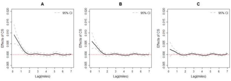
Estimated distributed lag coefficients quantifying association between availability of convenience stores up to 7 miles from schools and children’s BMIz: (A) crude; (B) with the adjustment of student characteristics, and (C) with the adjustment of both student and school’s characteristics. California 2009 Fitnessgram.
Table 2 compares the estimated average association between convenience stores up to 1/4, 1/2, 3/4, and 1 miles and children’s BMIz in the traditional linear and distributed lag models. In the crude analysis, the estimated average associations between the number of convenience stores up to 1/4, 1 /2, 3/4, or 1 miles were positive and had 95% CIs suggestive of associations for both the traditional linear and distributed lag models. In the results from the distributed lag model, BMIz was 0.009 (95% CI: [0.005; 0.013]) higher for each additional convenience store within 1/4 mile from schools. Adjusting for student characteristics alone, or for student and school characteristics, attenuated all coefficients. Overall, the coefficients from the traditional linear model tended to be larger (approximately 4 times larger or more) as may be expected given the bias observed in the simulations for these models in the presence of spatial correlation in the built environment.
Table 2.
Estimated associations between children’s BMIz and presence of one additional convenience store within buffer sizes ¼, ½, ¾, and 1 miles from schools, estimated with the traditional linear models (TLMs) and distributed lag models (DLMs). California 2009 Fitnessgram data.
| Model | Specified distance (rk) | TLMs | DLMs | ||
|---|---|---|---|---|---|
|
| |||||
| θ̂1,rk | 95% CI | β̄̂(0; rk) | 95% CI | ||
| Crude | 1/4 mile | 0.112 | [0.095; 0.129] | 0.009 | [0.005; 0.013] |
| 1/2 mile | 0.083 | [0.075; 0.090] | 0.008 | [0.005; 0.010] | |
| 3/4 mile | 0.056 | [0.052; 0.061] | 0.006 | [0.005; 0.008] | |
| 1 mile | 0.039 | [0.037; 0.042] | 0.005 | [0.004; 0.007] | |
|
| |||||
| Adjusted student characteristics | 1/4 mile | 0.059 | [0.044; 0.072] | 0.006 | [0.003; 0.009] |
| 1/2 mile | 0.043 | [0.037; 0.049] | 0.005 | [0.003; 0.007] | |
| 3/4 mile | 0.030 | [0.026; 0.033] | 0.004 | [0.003; 0.006] | |
| 1 mile | 0.020 | [0.018; 0.022] | 0.003 | [0.002; 0.005] | |
|
| |||||
| Adjusted student characteristics + school characteristics | 1/4 mile | 0.017 | [0.006; 0.028] | 0.002 | [-0.001; 0.005] |
| 1/2 mile | 0.013 | [0.008; 0.018] | 0.002 | [0.000; 0.004] | |
| 3/4 mile | 0.009 | [0.006; 0.013] | 0.002 | [0.000; 0.003] | |
| 1 mile | 0.006 | [0.004; 0.008] | 0.001 | [0.000; 0.002] | |
We investigated whether associations differed by grade (5th grade vs. 7th grade children), sex (girls vs. boys), and race/ethnicity (non-Hispanic Whites vs. Hispanics). We hypothesized that this would be the case since (1) 7th graders might have different behaviors and characteristics e.g., greater ability to walk farther distances and more pocket money, and (2) previous studies have observed differences by sex, and race/ethnicity.4 To assess this, we included in the model indicators of 7th grade, female sex, and Hispanic ethnicity in the school as interacting covariates. The associations did not differ by individual characteristics (eFigure 1).
DISCUSSION
We proposed using distributed lag modeling to examine associations between built environment factors and health outcomes. The distributed lag model approach is based on constructing environment measures within ring-shaped regions around sample locations, and constraining the coefficients to follow a smooth association over distance. The approach has the distinctive advantage of revealing how associations between features of the built environment and health are distributed across distances (up to a maximum distance) from locations of interest. Hence, distributed lag models can help generate empirical evidence regarding the most relevant spatial scales for a given health outcome and built environment attribute. For instance, because the distributed lag coefficients for convenience store availability in our BMIz case study become indistinguishable from zero at around 1 mile, 1 mile buffers rather than the widely used ½ mile buffer may be more appropriate for studies involving children’s exposure to convenience stores. Distributed lag models, however, do not require the use of pre-specified buffers. When average associations within a predetermined buffer size are of interest, distributed lag model coefficients can be used calculate them more accurately and with higher precision than commonly used traditional linear models.
Distributed lag models rely on specifying a maximum distance, beyond which we assume no association between the outcome and the built environment factors. Violation of this assumption might bias estimated distributed lag coefficients, since they would be confounded by associations with features beyond the maximum distance when spatial correlation exists in the built environment. While traditional approaches require speculating about the distance where effects may be present, distributed lag models’ single requirement is less stringent: specifying a distance beyond which there is no association and simultaneously permitting examination of whether these effects are indeed vanishing with distance.
In our case study, we examined the association between convenience store availability and children’s BMIz scores using data on 5th and 7th grade non-Hispanic White and Hispanic children using the 2009 FitnessGram surveillance data. In models adjusted for individual (and area) level factors, the magnitude of the distributed lag coefficients and their 95%CI suggested that convenience store availability within 1 mile from schools was associated with higher BMIz; associations did not differ by student characteristics (grade, sex, race/ethnicity). The associations, which only accounted for one feature of the environment, were relatively small magnitude and, though they may not be as meaningful at the individual level, they may be important at the population level.37 When comparing buffer associations between the models, we found that estimates using traditional linear models were usually higher than those from distributed lag models, possibly due to bias induced by spatial clustering of convenience stores.
Several extensions of the distributed lag model are possible, which would overcome some of its limitations. The distributed lag model assumes that relevant areas have a circular shape around schools; the circular shape provides comparability to results obtained using traditional methods and buffers around the outcome locations. Future work can construct areas around the outcome locations from shapes derived using street-network distances. The model proposed here estimated the overall association between the built environment and health, but did not examine how or if the association varies spatially across locations, although such extensions are possible38. Finally, although the distributed lag model approach breaks new ground by helping to explore the spatial scale of built environment effects, it does not fully capture the complexity of the built environment. Methodologic work is needed that permits consideration of several environmental features simultaneously, which may or may not be associated with each other or with the outcome at different spatial scales.
Future work should examine the relative performance of other methods to constrain distributed lag coefficients in the context of built environment data; we used smoothing splines since they are straightforward to implement in available software. Alternative methods that can reduce the estimated uncertainty in the first few lags (e.g, see Figure 4 and eFigure 2), which is due to a preponderance of zero features near locations of interest, should be explored. For instance, approaches are of interest that smooth differentially depending on the lag t.23 Smoothing the coefficients using Gaussian Process priors, previously compared to smoothing splines39 but not in the context of built environment data, may have the advantage of directly linking the amount of smoothing to the width of the rings where built environment features are counted (as suggested by an anonymous reviewer) thus potentially addressing issues related to zero counts within rings. Other Gaussian Process priors-based approaches may be used to directly estimate the most relevant buffer size.25 The utility of kernel-averaged predictor models, which formalize the idea that the observed outcome is likely to depend on the value of the covariate at the location of interest and on a weighted average of the covariate over an area centered around the location,40 should also be explored.
Although distributed lag models have a long history, to our knowledge this is the first application of these models to study built environment and health associations. This innovative application of distributed lag models can shed light on the relevant distances within which built environment features may affect health.
Supplementary Material
Acknowledgments
Sources of financial support:
The authors acknowledge salary support by grants from the National Heart, Lung, and Blood Institute of the National Institutes of Health: K01HL115471 (Sanchez-Vaznaugh), P01ES022844, P20ES018171, P60MD002249, and R01HL071759; and the Robert Wood Johnson Foundation: 69599. The content is solely the responsibility of the authors and does not necessarily represent the official views of those institutions.
Footnotes
Conflicts of interest: none.
References
- 1.Diez-Roux AV. Bringing context back into epidemiology: variables and fallacies in multilevel analysis. Am J Public Health. 1998;88:216–222. doi: 10.2105/ajph.88.2.216. [DOI] [PMC free article] [PubMed] [Google Scholar]
- 2.Susser M. The logic in ecological: I. The logic of analysis. Am J Public Health. 1994;84:825–829. doi: 10.2105/ajph.84.5.825. [DOI] [PMC free article] [PubMed] [Google Scholar]
- 3.Davis B, Carpenter C. Proximity of fast-food restaurants to schools and adolescent obesity. Am J Public Health. 2009;99:505–510. doi: 10.2105/AJPH.2008.137638. [DOI] [PMC free article] [PubMed] [Google Scholar]
- 4.Sánchez BN, Sanchez-Vaznaugh EV, Uscilka A, Baek J, Zhang L. Differential associations between the food environment near schools and childhood overweight across race/ethnicity, gender, and grade. Am J Epidemiol. 2012;175:1284–1293. doi: 10.1093/aje/kwr454. [DOI] [PMC free article] [PubMed] [Google Scholar]
- 5.Currie J, Dellavigna S, Moretti E, Pathania V. Working Paper No 14721. JEL No I1, I18, J0. Cambridge, MA: National Bureau of Economic Research; 2009. The effect of fast food restaurants on obesity and weight gain. [Google Scholar]
- 6.Harris DE, Blum JW, Bampton M, et al. Location of food stores near schools does not predict the weight status of Maine high school students. J Nutr Educ Behav. 2011;43:274–278. doi: 10.1016/j.jneb.2010.08.008. [DOI] [PubMed] [Google Scholar]
- 7.Langellier BA. The food environment and student weight status, Los Angeles County 2008-2009. Prev Chronic Dis. 2012;9:E61. [PMC free article] [PubMed] [Google Scholar]
- 8.Hillier A, Cole BL, Smith TE, et al. Clustering of unhealthy outdoor advertisements around child-serving institutions: a comparison of three cities. Health Place. 2009;15:935–945. doi: 10.1016/j.healthplace.2009.02.014. [DOI] [PubMed] [Google Scholar]
- 9.Gebauer H, Laska MN. Convenience stores surrounding urban schools: an assessment of healthy food availability, advertising, and product placement. J Urban Health. 2011;88:616–622. doi: 10.1007/s11524-011-9576-3. [DOI] [PMC free article] [PubMed] [Google Scholar]
- 10.Charreire H, Casey R, Salze P, et al. Measuring the food environment using geographical information systems: a methodological review. Public Health Nutr. 2010;13:1773–1785. doi: 10.1017/S1368980010000753. [DOI] [PubMed] [Google Scholar]
- 11.An R, Sturm R. School and residential neighborhood food environment and diet among California youth. Am J Prev Med. 2012;42:129–135. doi: 10.1016/j.amepre.2011.10.012. [DOI] [PMC free article] [PubMed] [Google Scholar]
- 12.Howard PH, Fitzpatrick M, Fulfrost B. Proximity of food retailers to schools and rates of overweight ninth grade students: an ecological study in California. BMC Public Health. 2011;11:68. doi: 10.1186/1471-2458-11-68. [DOI] [PMC free article] [PubMed] [Google Scholar]
- 13.Guo J, Bhat C. Modifiable areal units: problem or perception in modeling of residential location choice? Transp Res Rec. 2004;1898:138–147. [Google Scholar]
- 14.Spielman SE, Yoo EH. The spatial dimensions of neighborhood effects. Soc Sci Med. 2009;68:1098–1105. doi: 10.1016/j.socscimed.2008.12.048. [DOI] [PubMed] [Google Scholar]
- 15.Openshaw S. Chapter 4. Developing GIS-relevant zone-based spatial analysis methods. In: Longley P, Batty M, editors. spatial analysis: modelling in a GIS environment. Cambridge, England: Geoinformation International; 1996. [Google Scholar]
- 16.Fotheringham AS, Wong DWS. The modifiable areal unit problem in multivariate statistical analysis. Environ Plan A. 1991;23:1025–1044. [Google Scholar]
- 17.Koyck LM. Distributed Lags and Investment Analysis. Amsterdam: North-Holland; 1954. [Google Scholar]
- 18.Almon S. The distributed lag between capital appropriations and expenditures. Econom J Econom Soc. 1965;33:178–196. [Google Scholar]
- 19.Dominici F, McDermott A, Hastie TJ. Improved semiparametric time series models of air pollution and mortality. J Am Stat Assoc. 2004;468:938–948. [Google Scholar]
- 20.Pope CA, III, Dockery DW, Spengler JD, Raizenne ME. Respiratory health and PM 10 pollution. A daily time series analysis. Am Rev Respir Dis. 1991;144:668–674. doi: 10.1164/ajrccm/144.3_Pt_1.668. [DOI] [PubMed] [Google Scholar]
- 21.Pope CA, III, Schwartz J. Time series for the analysis of pulmonary health data. Am J Respir Crit Care Med. 1996;154(6 pt 2):S229–S233. doi: 10.1164/ajrccm/154.6_Pt_2.S229. [DOI] [PubMed] [Google Scholar]
- 22.Zanobetti A, Wand MP, Schwartz J, Ryan LM. Generalized additive distributed lag models : quantifying mortality displacement. Biostatistics. 2000;1:279–292. doi: 10.1093/biostatistics/1.3.279. [DOI] [PubMed] [Google Scholar]
- 23.Welty LJ, Peng RD, Zeger SL, Dominici F. Bayesian distributed lag models: estimating effects of particulate matter air pollution on daily mortality. Biometrics. 2009;65:282–291. doi: 10.1111/j.1541-0420.2007.01039.x. [DOI] [PubMed] [Google Scholar]
- 24.Goodman PG, Dockery DW, Clancy L. Cause-specific mortality and the extended effects of particulate pollution and temperature exposure. Environ Health Perspect. 2004;112:179–185. doi: 10.1289/ehp.6451. [DOI] [PMC free article] [PubMed] [Google Scholar]
- 25.Heaton MJ, Peng RD. Flexible distributed lag models using random functions with application to estimating mortality displacement from heat-related deaths. J Agric Biol Environ Stat. 2012;17:313–331. doi: 10.1007/s13253-012-0097-7. [DOI] [PMC free article] [PubMed] [Google Scholar]
- 26.Boone-Heinonen J, Gordon-Larsen P, Kiefe CI, Shikany JM, Lewis CE, Popkin BM. Fast food restaurants and food stores: longitudinal associations with diet in young to middle-aged adults: the CARDIA study. JAMA Intern Med. 2011;171:1162–1170. doi: 10.1001/archinternmed.2011.283. [DOI] [PMC free article] [PubMed] [Google Scholar]
- 27.Hastie TJ, Tibshirani RJ. Generalized Additive Models. Boca Raton, FL: CRC Press; 1990. [Google Scholar]
- 28.R Development Core Team. R: a language and environment for statistical computing, reference index version 3.0.1. Vienna, Austria: R Foundation for Statistical Computing; [May 5, 2011]. Available at https://www.r-project.org. [Google Scholar]
- 29.Gasparrini A. Distributed lag linear and non-linear models in R: The Package dlnm. J Stat Softw. 2011;43:1–20. [PMC free article] [PubMed] [Google Scholar]
- 30.Lunn DJ, Thomas A, Best N, Spiegelhalter D. WinBUGS – A Bayesian modelling framework: Concepts, structure, and extensibility. Stat Comput. 2000;10:325–337. [Google Scholar]
- 31.Montgomery DC, Peck EA, Vining GG. Introduction to Linear Regression Analysis. 5. NY: Wiley; 2012. [Google Scholar]
- 32.Sanchez-Vaznaugh EV, Sanchez BN, Baek J, Crawford PB. Competitive food and beverage policies: are they influencing childhood overweight trends? Health Aff (Millwood) 2010;29:436–446. doi: 10.1377/hlthaff.2009.0745. [DOI] [PubMed] [Google Scholar]
- 33.Walls & Associates. [April 5, 2015];National Establishment Time-Series (NETS) Database. Available at http://exceptionalgrowth.org/our-databases.iegc.
- 34.Diez-Roux AV. Estimating neighborhood health effects: the challenges of causal inference in a complex world. Soc Sci Med. 2004;58:1953–1960. doi: 10.1016/S0277-9536(03)00414-3. [DOI] [PubMed] [Google Scholar]
- 35.Chaix B, Leal C, Evans D. Neighborhood-level confounding in epidemiologic studies: unavoidable challenges, uncertain solutions. Epidemiology. 2010;21:124–127. doi: 10.1097/EDE.0b013e3181c04e70. [DOI] [PubMed] [Google Scholar]
- 36.Spiegelhalter DJ, Best NG, Carlin BP, Van Der Linde A. Bayesian measures of model complexity and fit. J R Stat Soc Series B Stat Methodol. 2002;64:583–639. [Google Scholar]
- 37.Rose G. Sick individuals and sick populations. Int J Epidemiol. 2001;30:990–996. doi: 10.1093/ije/30.3.427. [DOI] [PubMed] [Google Scholar]
- 38.Baek J. Dissertation. 2014. Statistical models to assess associations between the built environment and health: examining food environment contributions to the child obesity epidemic. [Google Scholar]
- 39.Kimeldorf GS, Wahba G. A correspondence between Bayesian estimation on stochastic processes and smoothing by splines. Ann Math Stat. 1970;41:495–502. [Google Scholar]
- 40.Heaton MJ, Gelfand AE. Spatial regression using kernel averaged predictors. J Agric Biol Environ Stat. 2011;16:233–252. [Google Scholar]
Associated Data
This section collects any data citations, data availability statements, or supplementary materials included in this article.