

Abstract
Effective population size characterizes the genetic variability in a population and is a parameter of paramount importance in population genetics and evolutionary biology. Kingman’s coalescent process enables inference of past population dynamics directly from molecular sequence data, and researchers have developed a number of flexible coalescent-based models for Bayesian nonparametric estimation of the effective population size as a function of time. Major goals of demographic reconstruction include identifying driving factors of effective population size, and understanding the association between the effective population size and such factors. Building upon Bayesian nonparametric coalescent-based approaches, we introduce a flexible framework that incorporates time-varying covariates that exploit Gaussian Markov random fields to achieve temporal smoothing of effective population size trajectories. To approximate the posterior distribution, we adapt efficient Markov chain Monte Carlo algorithms designed for highly structured Gaussian models. Incorporating covariates into the demographic inference framework enables the modeling of associations between the effective population size and covariates while accounting for uncertainty in population histories. Furthermore, it can lead to more precise estimates of population dynamics. We apply our model to four examples. We reconstruct the demographic history of raccoon rabies in North America and find a significant association with the spatiotemporal spread of the outbreak. Next, we examine the effective population size trajectory of the DENV-4 virus in Puerto Rico along with viral isolate count data and find similar cyclic patterns. We compare the population history of the HIV-1 CRF02_AG clade in Cameroon with HIV incidence and prevalence data and find that the effective population size is more reflective of incidence rate. Finally, we explore the hypothesis that the population dynamics of musk ox during the Late Quaternary period were related to climate change. [Coalescent; effective population size; Gaussian Markov random fields; phylodynamics; phylogenetics; population genetics.
The effective population size is an abstract parameter of fundamental importance in population genetics, evolutionary biology, and infectious disease epidemiology. Wright (1931) introduces the concept of effective population size as the size of an idealized Fisher–Wright population that gains and loses genetic diversity at the same rate as the real population under study. The Fisher–Wright model is a classic forward-time model of reproduction that assumes random mating, no selection or migration, and nonoverlapping generations. Coalescent theory (Kingman 1982a, 1982b) provides a probabilistic model for generating genealogies relating samples of individuals arising from a Fisher–Wright model of reproduction. Importantly, the coalescent elucidates the relationship between population genetic parameters and ancestry. In particular, the dynamics of the effective population size greatly inform the shapes of coalescent-generated genealogies. This opens the door for the inverse problem of coalescent-based inference of effective population size trajectories from gene genealogies.
While the coalescent was originally developed for constant-size populations, extensions that accommodate a variable population size (Slatkin and Hudson 1991; Griffiths and Tavaré 1994; Donnelly and Tavaré 1995) provide a basis for estimation of the effective population size as a function of time (also called the demographic function). Early approaches assumed simple parametric forms for the demographic function, such as exponential or logistic growth, and provided maximum likelihood (Kuhner et al. 1998) or Bayesian (Drummond et al. 2002) frameworks for estimating the parameters that characterized the parametric forms. However, a priori parametric assumptions can be quite restrictive, and finding an appropriate parametric form for a given demographic history can be time consuming and computationally expensive. To remedy this, there has been considerable development of nonparametric methods to infer past population dynamics.
Nonparametric coalescent-based models typically approximate the effective population size as a piecewise constant or linear function. The methodology has evolved from fast but noisy models based on method of moments estimators (Pybus et al. 2000; Strimmer and Pybus 2001), to a number of flexible Bayesian approaches, including multiple change-point models (Drummond et al. 2005; Opgen-Rhein et al. 2005; Heled and Drummond 2008), and models that employ Gaussian process-based priors on the population trajectory (Minin et al. 2008; Gill et al. 2013; Palacios and Minin 2013). Extending the basic methodological framework to incorporate a number of key features, including accounting for phylogenetic error (Drummond et al. 2005; Heled and Drummond 2008; Minin et al. 2008; Gill et al. 2013), the ability to analyze heterochronous data (Pybus et al. 2000; Drummond et al. 2005; Heled and Drummond 2008; Minin et al. 2008; Gill et al. 2013; Palacios and Minin 2013), and simultaneous analysis of multilocus data (Heled and Drummond 2008; Gill et al. 2013) has hastened progress.
In spite of all of these advances, there remains a need for further development of population dynamics inference methodology. One promising avenue is introduction of covariates into the inference framework. A central goal in demographic reconstruction is to gain insights into the association between past population dynamics and external factors (Ho and Shapiro 2011). For example, Lorenzen et al. (2011) combine demographic reconstructions from ancient DNA with species distribution models and the human fossil record to elucidate how climate and humans impacted the population dynamics of woolly rhinoceros, woolly mammoth, wild horse, reindeer, bison, and musk ox during the Late Quaternary period. Lorenzen et al. (2011) show that changes in megafauna abundance are idiosyncratic, with different species (and continental populations within species) responding differently to the effects of climate change, human encroachment and habitat redistribution. Lorenzen et al. (2011) identify climate change as the primary explanation behind the extinction of Eurasian musk ox and woolly rhinoceros, point to a combination of climatic and anthropogenic factors as the causes of wild horse and steppe bison decline, and observe that reindeer remain largely unaffected by any such factors. Similarly, Stiller et al. (2010) examine whether climatic changes were related to the extinction of the cave bear, and Finlay et al. (2007) consider the impact of domestication on the population expansion of bovine species. Comparison of external factors with past population dynamics is also a popular approach in epidemiological studies to explore hypotheses about the spread of viruses (Lemey et al. 2003; Faria et al. 2014).
In addition to the association between past population dynamics and potential driving factors, it is of fundamental interest to assess the association between effective population size and census population size (Crandall et al. 1999; Liu and Mittler 2008; Volz et al. 2009; Palstra and Fraser 2012). For instance, Bazin et al. (2006) argue that in animals, diversity of mitochondrial DNA (mtDNA) is not reflective of population size, whereas allozyme diversity is. Atkinson et al. (2008) follow up by examining whether mtDNA diversity is a reliable predictor of human population size. The authors compare Bayesian Skyline (Drummond et al. 2005) effective population size reconstructions with historical estimates of census population sizes and find concordance between the two quantities in terms of relative regional population sizes.
Existing methods for population dynamics inference do not incorporate covariates directly into the model, and associations between the effective population size and potentially related factors are typically examined in post hoc fashions that ignore uncertainty in demographic reconstructions. We propose to fill this void by including external time series as covariates in a generalized linear model (GLM) framework. We accomplish this task by building upon the Bayesian nonparametric Skygrid model of Gill et al. (2013). The Skygrid is a particularly well-suited starting point among nonparametric coalescent-based models. In most other comparable models, the trajectory change-points must correspond to internal nodes of the genealogy, creating a hurdle for modeling associations with covariates that are measured at fixed times. The Skygrid bypasses such difficulties by allowing users to specify change-points, providing a more natural framework for our extension. Furthermore, the Skygrid’s Gaussian Markov random field (GMRF) smoothing prior is highly generalizable and affords a straightforward extension to include covariates.
We demonstrate the utility of incorporating covariates into demographic inference on four examples. First, we find striking similarities between the demographic and spatial expansion of raccoon rabies in North America. Second, we compare and contrast the epidemiological dynamics of dengue in Puerto Rico with patterns of viral diversity. Third, we examine the population history of the HIV-1 CRF02_AG clade in Cameroon and find that the effective population size is more reflective of HIV incidence than prevalence. Finally, we explore the relationship between musk ox population dynamics and climate change during the Late Quaternary period. Our extension to the Skygrid proves to be a useful framework for ascertaining the association between effective population size and external covariates while accounting for demographic uncertainty. Furthermore, we show that incorporating covariates into the demographic inference framework can improve estimates of effective population size trajectories, increasing precision and uncovering patterns in the population history that integrate the covariate data in addition to the sequence data.
Methods
We begin with an overview of coalescent theory and follow with a detailed development of the Skygrid inference framework before presenting its extension that incorporates external covariate data. Readers interested in previewing our approach to include covariates may skip to the section Incorporating Covariates. However, we encourage readers who are unfamiliar with the Skygrid to proceed in order.
Coalescent Theory
Consider a random sample of  individuals
arising from a classic Fisher–Wright population model of constant size
individuals
arising from a classic Fisher–Wright population model of constant size
 . The coalescent (Kingman 1982a, 1982b) is a stochastic process that generates genealogies relating such a
sample. The process begins at the sampling time of all
. The coalescent (Kingman 1982a, 1982b) is a stochastic process that generates genealogies relating such a
sample. The process begins at the sampling time of all  individuals,
  , and proceeds backward in time
as
, and proceeds backward in time
as  increases, successively merging
lineages until all lineages have merged and we have reached the root of the
genealogy, which corresponds to the most recent common ancestor (MRCA) of the sampled
individuals. The merging of lineages is called a coalescent event and there are
increases, successively merging
lineages until all lineages have merged and we have reached the root of the
genealogy, which corresponds to the most recent common ancestor (MRCA) of the sampled
individuals. The merging of lineages is called a coalescent event and there are
 coalescent events in all. Let
 denote the time of the
 -th coalescent event for
 and
and
 denote the sampling time.
Then for
denote the sampling time.
Then for  , the waiting time
 is exponentially
distributed with rate
is exponentially
distributed with rate  .
.
Researchers have extended coalescent theory to model the effects of recombination
(Hudson 1983), population structure (Notohara 1990), and selection (Krone and Neuhauser 1997). We do not, however,
incorporate any of these extensions here. The relevant extensions for our development
generalize the coalescent to accommodate a variable population size (Griffiths and Tavaré 1994) and
heterochronous data (Rodrigo and Felsenstein
1999). The latter occurs when the  individuals are sampled at two or more different times.
Let  denote the effective
population size as a function of time, where time increases into the past. Thus,
denote the effective
population size as a function of time, where time increases into the past. Thus,
 is the effective population
size at the most recent sampling time, and
is the effective population
size at the most recent sampling time, and  is the
effective population size
is the
effective population size  time units
before the most recent sampling time. We also refer to
time units
before the most recent sampling time. We also refer to  as the “demographic
function” or “demographic model.” Griffiths and Tavaré (1994) show that the waiting time
as the “demographic
function” or “demographic model.” Griffiths and Tavaré (1994) show that the waiting time
 between coalescent events is
given by the conditional density
between coalescent events is
given by the conditional density
| (1) |
Taking the product of such densities yields the joint density of intercoalescent waiting times, and this fact can be exploited to obtain the probability of observing a particular genealogy given a demographic function.
Skygrid Demographic Model
The Skygrid posits that  is a piecewise constant
function that can change values only at pre-specified points in time known as
“grid points.” Let
is a piecewise constant
function that can change values only at pre-specified points in time known as
“grid points.” Let  denote the temporal grid points, where
  .
The
.
The  grid points divide the demographic
history timeline into
grid points divide the demographic
history timeline into  intervals so that the
demographic function is fully specified by a vector
intervals so that the
demographic function is fully specified by a vector  of values that it assumes on those intervals. Here,
  for
for
 ,
,
 , where it is
understood that
, where it is
understood that  . Also,
 for
for
 . Note that
 is the time furthest back into
the past at which the effective population size can change. The values of the grid
points as well as the number
is the time furthest back into
the past at which the effective population size can change. The values of the grid
points as well as the number  of total grid
points are specified beforehand by the user. A typical way to select the grid points
is to decide on a resolution
of total grid
points are specified beforehand by the user. A typical way to select the grid points
is to decide on a resolution  , let
, let
 assume the value furthest back
in time for which the data are expected to be informative, and space the remaining
grid points evenly between
assume the value furthest back
in time for which the data are expected to be informative, and space the remaining
grid points evenly between  and
and
 . Alternatively, as discussed in
the next section, grid points can be selected to align with covariate sampling times
to facilitate the modeling of associations between the effective population size and
external covariates.
. Alternatively, as discussed in
the next section, grid points can be selected to align with covariate sampling times
to facilitate the modeling of associations between the effective population size and
external covariates.
Suppose we have  known genealogies
 representing the
ancestries of samples from
representing the
ancestries of samples from  separate genetic
loci with the same effective population size
separate genetic
loci with the same effective population size  . We assume a
priori that the genealogies are independent given
. We assume a
priori that the genealogies are independent given
 . This assumption implies that
the genealogies are unlinked which commonly occurs when researchers select loci from
whole genome sequences or when recombination is very likely, such as between genes in
retroviruses. The likelihood of the vector
. This assumption implies that
the genealogies are unlinked which commonly occurs when researchers select loci from
whole genome sequences or when recombination is very likely, such as between genes in
retroviruses. The likelihood of the vector  of
genealogies can then be expressed as the product of likelihoods of individual
genealogies:
of
genealogies can then be expressed as the product of likelihoods of individual
genealogies:
| (2) |
To construct the likelihood of genealogy  , let
, let
 be the most recent sampling
time of sequences contributing to genealogy
be the most recent sampling
time of sequences contributing to genealogy  and
and  be the time of
the MRCA for locus
be the time of
the MRCA for locus  . Let
. Let  denote the minimal grid
point greater than at least one sampling time in the genealogy, and
denote the minimal grid
point greater than at least one sampling time in the genealogy, and
 the greatest grid point
less than at least one coalescent time. Let
the greatest grid point
less than at least one coalescent time. Let  ,
,
 ,
,
 ,
and
,
and  .
For each
.
For each  we let
 ,
,  , denote the ordered times
of the grid points and sampling and coalescent events in the interval. With each
, denote the ordered times
of the grid points and sampling and coalescent events in the interval. With each
 we associate an indicator
 which takes a value of 1
in the case of a coalescent event and 0 otherwise. Finally, let
which takes a value of 1
in the case of a coalescent event and 0 otherwise. Finally, let
 denote the number of lineages
present in the genealogy in the interval
denote the number of lineages
present in the genealogy in the interval  . Following Griffiths and Tavaré (1994), the
likelihood of observing an interval is
. Following Griffiths and Tavaré (1994), the
likelihood of observing an interval is
| (3) |
for  .
.
The product of interval likelihoods (3) yields the likelihood of coalescent times given the sampling times
associated with genealogy  . However,
identical coalescent times can arise from distinct genealogies. Immediately prior to
a coalescent time
. However,
identical coalescent times can arise from distinct genealogies. Immediately prior to
a coalescent time  , there are
 distinct lineages and,
therefore,
distinct lineages and,
therefore,  different
pairs of lineages that can merge and result in a coalescent event at time
different
pairs of lineages that can merge and result in a coalescent event at time
 . The different possible
mergings correspond to different genealogies. To obtain the likelihood of a
particular genealogy we must account for the fact that a specific pair of lineages
must merge at each coalescent time. Let
. The different possible
mergings correspond to different genealogies. To obtain the likelihood of a
particular genealogy we must account for the fact that a specific pair of lineages
must merge at each coalescent time. Let  denote
 except with
factors of the form
except with
factors of the form  replaced by
  .
Then,
.
Then,
| (4) |
We introduce some notation that will facilitate the derivation of a Gaussian
approximation used to construct a Markov chain Monte Carlo (MCMC) transition kernel.
If  denotes the number of
coalescent events which occur during interval
denotes the number of
coalescent events which occur during interval  , we can write
| (5) |
where the  are
appropriate constants. Rewriting this expression in terms of
are
appropriate constants. Rewriting this expression in terms of
 , we arrive
at
, we arrive
at
| (6) |
Invoking conditional independence of genealogies, the likelihood of the vector
 of genealogies is
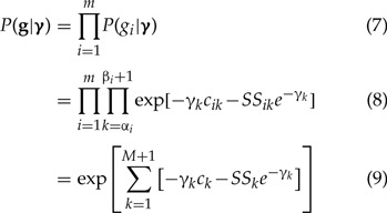 |
where  and
and
 ;
here,
;
here,  if
if
 .
.
The Skygrid incorporates the prior assumption that effective population size changes
continuously over time by placing a GMRF prior on  :
:
| (10) |
This prior does not inform the overall level of the effective population size, just
the smoothness of the trajectory. One can think of the prior as a first-order
unbiased random walk with normal increments. The precision parameter
 determines how much differences
between adjacent log effective population size values are penalized. We assign
determines how much differences
between adjacent log effective population size values are penalized. We assign
 a gamma prior:
| (11) |
In the absence of prior knowledge about the smoothness of the effective population
size trajectory, we choose  so
that it is relatively uninformative. Conditioning on the vector of genealogies, we
obtain the posterior distribution
so
that it is relatively uninformative. Conditioning on the vector of genealogies, we
obtain the posterior distribution
| (12) |
Incorporating Covariates
We can incorporate covariates into our inference framework by adopting a GLM
approach. Let  be a set of
 predictors. Each covariate
 is observed or measured at
 time points,
 . Here,
 denotes the units of time before
the most recent sequence sampling time
denotes the units of time before
the most recent sequence sampling time  , and
, and
 .
Alternatively, the covariate may correspond to time intervals
.
Alternatively, the covariate may correspond to time intervals
 rather than time points (e.g., the yearly incidence or prevalence of viral
infections). In any case,
rather than time points (e.g., the yearly incidence or prevalence of viral
infections). In any case,  denotes
covariate
denotes
covariate  at time point or interval
 . Skygrid grid points are chosen to
match up with measurement times (or measurement interval endpoints):
. Skygrid grid points are chosen to
match up with measurement times (or measurement interval endpoints):
 . Then
 for
for
 ,
,
 , and
, and
 for
for
 . In our GLM framework, we
model the effective population size on a given interval as a log-linear function of
covariates
. In our GLM framework, we
model the effective population size on a given interval as a log-linear function of
covariates
| (13) |
Here, we can impose temporal dependence by modeling  as a
zero-mean Gaussian process. Adopting this viewpoint, we propose the following GMRF
smoothing prior on
as a
zero-mean Gaussian process. Adopting this viewpoint, we propose the following GMRF
smoothing prior on  :
:
| (14) |
In this prior,  is an
is an
 matrix of covariates
and
matrix of covariates
and  is a
is a
 vector of coefficients
representing the effect sizes for the predictors, quantifying their contribution to
vector of coefficients
representing the effect sizes for the predictors, quantifying their contribution to
 . Precision
 is an
is an
 tri-diagonal
matrix with off-diagonal elements equal to
tri-diagonal
matrix with off-diagonal elements equal to  ,
,
 , and
, and
 for
for
 . Let
. Let
 denote the
vector obtained by excluding only the
denote the
vector obtained by excluding only the  -th component
from vector
-th component
from vector  . Therefore,
conditional on
. Therefore,
conditional on  ,
,
 depends only on its
immediate neighbors. Let
depends only on its
immediate neighbors. Let  denote
the
denote
the  -th row of covariate matrix
 . The individual components
of
. The individual components
of  have full conditionals
| (15) |
| (16) |
| (17) |
As in the original Skygrid GMRF prior, the precision parameter
 governs the smoothness of the
trajectory and is assigned a gamma prior
governs the smoothness of the
trajectory and is assigned a gamma prior
| (18) |
To complete the model specification, we place a relatively uninformative multivariate
normal prior  on the
coefficients
on the
coefficients  . This yields the
posterior
. This yields the
posterior
| (19) |
Missing Covariate Data
It is important to have a mechanism for dealing with unobserved covariate values.
This is particularly crucial because the population history timeline, which ranges
from the most recent sampling time to the time of the MRCA, necessitates observations
from a wide and a priori unknown time span. Let
 denote the
observed covariate values and
denote the
observed covariate values and  the missing
covariate values, so that
the missing
covariate values, so that  .
The missing data can be treated as extra unknown parameters in a Bayesian model, and
they can be estimated provided that there is a model that links them to the observed
data and other model parameters. We have the factorization
.
The missing data can be treated as extra unknown parameters in a Bayesian model, and
they can be estimated provided that there is a model that links them to the observed
data and other model parameters. We have the factorization
| (20) |
and the marginal density  can be recovered by integrating out the missing data. As a starting point, we assume
a “missing completely at random” structure, meaning that the
probability that a covariate value is missing is independent of observed covariate
values and other model parameters. For the priors on missing covariate values in
(20), we can adopt uniform
distributions over plausible ranges.
can be recovered by integrating out the missing data. As a starting point, we assume
a “missing completely at random” structure, meaning that the
probability that a covariate value is missing is independent of observed covariate
values and other model parameters. For the priors on missing covariate values in
(20), we can adopt uniform
distributions over plausible ranges.
Alternatively, we can formulate a prior on the missing covariate data that makes use
of the observed covariate values. Here, we focus on a common scenario where covariate
 is observed at times
 and unobserved at
times
and unobserved at
times  . Thus, we
can write
. Thus, we
can write  and
and  .
We model the joint distribution of the observed and missing covariate values as
multivariate normal,
.
We model the joint distribution of the observed and missing covariate values as
multivariate normal,
| (21) |
where
| (22) |
is the precision matrix. To impose a correlation structure that enforces dependence between covariate values corresponding to adjacent times, we adopt a first-order random walk with full conditionals
| (23) |
| (24) |
| (25) |
Let  denote a vector of
dimension
denote a vector of
dimension  with every entry equal to
 . Then the distribution of
missing covariate values conditional on observed covariate values is
. Then the distribution of
missing covariate values conditional on observed covariate values is
| (26) |
where
| (27) |
This technique of positing a random walk covariate distribution and recovering appropriate conditional distributions can also be employed for other missing data patterns.
MCMC Sampling Scheme
We use MCMC sampling to approximate the posterior
| (28) |
To sample  and
and
 , we propose a fast-mixing,
block-updating MCMC sampling scheme for GMRFs (Knorr-Held and Rue 2002). Suppose we have current parameter values
, we propose a fast-mixing,
block-updating MCMC sampling scheme for GMRFs (Knorr-Held and Rue 2002). Suppose we have current parameter values
 .
First, consider the full conditional density
.
First, consider the full conditional density
| (29) |
Let  .
We can approximate each term
.
We can approximate each term  by
a second-order Taylor expansion about, say,
by
a second-order Taylor expansion about, say,  :
:
| (30) |
We center the Taylor expansion about a point  obtained iteratively by the Newton–Raphson method:
| (31) |
with  ,
the current value of
,
the current value of  . Here,
| (32) |
with
| (33) |
and
| (34) |
Replacing the terms  with their Taylor
expansions yields the following second-order Gaussian approximation to the full
conditional density
with their Taylor
expansions yields the following second-order Gaussian approximation to the full
conditional density  :
:
| (35) |
where  is a diagonal matrix.
Starting from current parameter values  ,
we first generate a candidate value for the precision,
,
we first generate a candidate value for the precision,  , where
 is drawn from a symmetric proposal
distribution with density
is drawn from a symmetric proposal
distribution with density  defined on
 . The tuning constant
 controls the distance between the
proposed and current values of the precision. Next, conditional on
controls the distance between the
proposed and current values of the precision. Next, conditional on
 , we propose a new state
 using the
Gaussian approximation (35) to
the full conditional density
using the
Gaussian approximation (35) to
the full conditional density  .
In the final step, the candidate state
.
In the final step, the candidate state  is
accepted or rejected according to the Metropolis–Hastings ratio (Metropolis et al. 1953; Hastings 1970).
is
accepted or rejected according to the Metropolis–Hastings ratio (Metropolis et al. 1953; Hastings 1970).
Genealogical Uncertainty
In our development thus far, we have assumed the genealogies
 are known and fixed.
However, in reality we observe sequence data rather than genealogies. It is possible
to estimate genealogies beforehand from sequence data and then infer the effective
population size from fixed genealogies. However, this ignores the uncertainty
associated with phylogenetic reconstruction. Alternatively, we can jointly infer
genealogies and population dynamics from sequence data by combining the estimation
procedures into a single Bayesian framework.
are known and fixed.
However, in reality we observe sequence data rather than genealogies. It is possible
to estimate genealogies beforehand from sequence data and then infer the effective
population size from fixed genealogies. However, this ignores the uncertainty
associated with phylogenetic reconstruction. Alternatively, we can jointly infer
genealogies and population dynamics from sequence data by combining the estimation
procedures into a single Bayesian framework.
We can think of the aligned sequence data  for the
 loci as arising from
continuous-time Markov chain (CTMC) models for molecular character substitution that
act along the hidden genealogies. Each CTMC depends on a vector of mutational
parameters
loci as arising from
continuous-time Markov chain (CTMC) models for molecular character substitution that
act along the hidden genealogies. Each CTMC depends on a vector of mutational
parameters  , that include, for
example, an overall rate multiplier, relative exchange rates among characters and
across-site variation specifications. We let
, that include, for
example, an overall rate multiplier, relative exchange rates among characters and
across-site variation specifications. We let  .
We then jointly estimate the genealogies, mutational parameters, covariate effect
size coefficients, precision, and vector of effective population sizes through their
posterior distribution
.
We then jointly estimate the genealogies, mutational parameters, covariate effect
size coefficients, precision, and vector of effective population sizes through their
posterior distribution
| (36) |
Here, the coalescent acts as a prior for the genealogies, and we assume that
 and
and
 are a
priori independent of each other. Hierarchical models are, however,
available to share information about
are a
priori independent of each other. Hierarchical models are, however,
available to share information about  among loci without
strictly enforcing that they follow the same evolutionary process (Suchard et al. 2003; Edo-Matas et al. 2011). We implement our models in the
open-source software program BEAST v1 (Drummond et
al. 2012). The posterior distribution is approximated through MCMC methods.
We combine our block-updating scheme for
among loci without
strictly enforcing that they follow the same evolutionary process (Suchard et al. 2003; Edo-Matas et al. 2011). We implement our models in the
open-source software program BEAST v1 (Drummond et
al. 2012). The posterior distribution is approximated through MCMC methods.
We combine our block-updating scheme for  and
and  with standard transition
kernels available in BEAST to update the other parameters. The extended Skygrid model
will be included in the next official release of BEAST v1. In the meantime, it can be
accessed by users through the BEAST v1 development branch source code, which is
available at https://github.com/beast-dev/beast-mcmc/. Example BEAST XML input
files are available as part of the Supplementary Material available on Dryad at
http://dx.doi.org/10.5061/dryad.mj0hn.
with standard transition
kernels available in BEAST to update the other parameters. The extended Skygrid model
will be included in the next official release of BEAST v1. In the meantime, it can be
accessed by users through the BEAST v1 development branch source code, which is
available at https://github.com/beast-dev/beast-mcmc/. Example BEAST XML input
files are available as part of the Supplementary Material available on Dryad at
http://dx.doi.org/10.5061/dryad.mj0hn.
Empirical Examples
Expansion in Epizootic Rabies Virus
Rabies is a zoonotic disease caused by the rabies virus, and is responsible for over 50,000 human deaths annually. In over 99% of human cases, the rabies virus is transmitted by dogs. However, there are a number of other important rabies reservoirs, such as bats and several terrestrial carnivore species, including raccoons (WHO 2015b). Epizootic rabies among raccoons was first identified in the United States in Florida in the 1940s, and the affected area of the subsequent expansion was limited to the southeastern United States (Kappus et al. 1970). A second focus of rabies among raccoons emerged in West Virginia in the late 1970s due to the translocation of raccoons incubating rabies from the southeastern United States The virus spread rapidly along the mid-Atlantic coast and northeastern United States over the following decades, and is one of the largest documented outbreaks in the history of wildlife rabies (Childs et al. 2000).
Biek et al. (2007) examine the population dynamics of the rabies epizootic among raccoons in the northeastern United States starting in the late 1970s. In a spatiogenetic analysis, Biek et al. (2007) compare a coalescent-based Bayesian Skyline estimate (Drummond et al. 2005) of the demographic history to the spatial expansion of the epidemic. In a post hoc approach, the authors find very similar temporal dynamics between the effective population size and the 15-month moving average of the area (in square kilometers) of counties newly affected by the rabies outbreak each month. The effective population size exhibits stages of moderate and rapid growth, as well as plateau periods with little or no growth. Population expansion coincides with time periods during which the virus invades new areas at a generally increasing rate. On the other hand, the effective population size shows little, if any, growth during periods when the virus invades new areas at a declining rate. Notably, Biek et al. (2007) demonstrate through their analysis that the largest contribution to the population expansion comes from the wave front, highlighting the degree to which the overall viral dynamics depend on processes at the wave front. We observe the same trends in a Skygrid demographic reconstruction based on the Biek et al. (2007) sequence data (Fig. 1).
Figure 1.

Skygrid demographic reconstruction of raccoon rabies epidemic in the northeastern United States. The gray line is the posterior mean log effective population size trajectory estimated only from sequence data without incorporating covariate data. The shaded gray region is the 95% BCI region for the log effective population size. The black line represents the covariate, the 15-month moving average of the log-transformed area of all counties newly affected by the raccoon rabies virus each month.
We build upon the analysis of Biek et al.
(2007) by incorporating the spatiotemporal spread of rabies into the
demographic inference model through the Skygrid. The sequence data consist of 47
sequences sampled from rabid raccoons between 1982 and 2004. They encompass the
complete rabies nucleoprotein ( ) genes as well
as large portions of the glycoprotein (
) genes as well
as large portions of the glycoprotein ( ) genes. As a
covariate, we initially adopt the 15-month moving average of the log-transformed area
of all counties newly affected by the raccoon rabies virus each month from 1977 to
1999 (Biek et al. 2007). We infer a posterior
mean covariate effect size of 0.24 with a 95% 0.77, 1.27),
implying that there is not a significant association between the log effective
population size and the covariate. This is not surprising, considering the patterns
of growth and decline in the covariate compared with the essentially monotonic trend
in the log effective population size (Fig.
1).
) genes. As a
covariate, we initially adopt the 15-month moving average of the log-transformed area
of all counties newly affected by the raccoon rabies virus each month from 1977 to
1999 (Biek et al. 2007). We infer a posterior
mean covariate effect size of 0.24 with a 95% 0.77, 1.27),
implying that there is not a significant association between the log effective
population size and the covariate. This is not surprising, considering the patterns
of growth and decline in the covariate compared with the essentially monotonic trend
in the log effective population size (Fig.
1).
Graphically comparing the rate at which the virus invades new areas with population dynamics clearly illustrates the relationship between the demographic and spatial expansion of the raccoon rabies outbreak. In modeling the association between the population dynamics and a covariate, however, we relate the covariate to the total effective population size (as opposed to the change in the effective population size). In this case, the cumulative affected area is a more suitable covariate than the newly affected area. We conduct an additional Skygrid analysis and use the log transform of the cumulative area (in square kilometers) of counties affected by raccoon rabies at various time points between 1977 and 1999 as a covariate. The area of a county is added to the cumulative total for the month during which rabies is first reported in that county. There are 175 months for which the cumulative affected area changes, and we specify the grid points to coincide with these change-points.
The Skygrid analysis with the log cumulative affected area covariate yields a
posterior mean estimate of 1.30 for the coefficient  , with a
95% BCI of (0.18, 2.86), implying a
significant, positive association between the effective population size of the
raccoon rabies virus and the cumulative area affected by the outbreak (Fig. 2). Periods of demographic expansion are
marked by relatively rapid rates of increase in the affected area, whereas plateaus
in the effective population size coincide with more modest rates of increase in the
affected area. The effective population size trajectory estimated from both sequence
and covariate data displays nearly identical patterns to the trajectory estimated
only from sequence data, except from 1990 to 1996, when its rate of increase is more
modest. Notably, the dark gray BCI region inferred from the sequence and covariate
data is narrower than and virtually entirely contained within the light gray BCI
region inferred only from the sequence data. Thus including the covariate in this
analysis not only yields an estimate consistent with what we infer from the sequence
data alone, but also a more precise estimate.
, with a
95% BCI of (0.18, 2.86), implying a
significant, positive association between the effective population size of the
raccoon rabies virus and the cumulative area affected by the outbreak (Fig. 2). Periods of demographic expansion are
marked by relatively rapid rates of increase in the affected area, whereas plateaus
in the effective population size coincide with more modest rates of increase in the
affected area. The effective population size trajectory estimated from both sequence
and covariate data displays nearly identical patterns to the trajectory estimated
only from sequence data, except from 1990 to 1996, when its rate of increase is more
modest. Notably, the dark gray BCI region inferred from the sequence and covariate
data is narrower than and virtually entirely contained within the light gray BCI
region inferred only from the sequence data. Thus including the covariate in this
analysis not only yields an estimate consistent with what we infer from the sequence
data alone, but also a more precise estimate.
Figure 2.

Demographic history of raccoon rabies epidemic in the northeastern United States. The black line that extends outside the shaded regions represents the covariate, the log cumulative area of counties affected by raccoon rabies virus. The black line contained within the shaded regions is the posterior mean log effective population size trajectory from the Skygrid analysis with the covariate, and the surrounding shaded dark gray region is its 95% BCI region. The white line is the posterior mean log effective population size trajectory from the Skygrid analysis without the covariate, and the surrounding shaded light gray region is its 95% BCI region. The two BCI regions overlap considerably, and the dark gray BCI region is almost entirely contained within the light gray BCI region.
Epidemic Dynamics in Dengue Evolution
Dengue is a mosquito-borne viral infection that causes a severe flu-like illness in which potentially lethal syndromes occasionally arise. Dengue is caused by the dengue virus, DENV, an RNA virus which comes in four antigenically distinct but closely related serotypes, DENV-1 through DENV-4. (WHO 2015a). A recent estimate places the worldwide burden of dengue at 390 million infections per year (with 95% confidence interval 284–528 million), of which 96 million (67–136 million) manifest clinically (with any level of disease severity) (Bhatt et al. 2013). Dengue is found in tropical and sub-tropical climates throughout the world, mostly in urban and semi-urban areas (WHO 2015a).
Dengue incidence records often show patterns of periodicity with outbreaks every 3–5 years (Cummings et al. 2004; Adams et al. 2006; Bennett et al. 2010). Studies have shown that the epidemiological dynamics of dengue transmission in Puerto Rico are reflective of changes in the viral effective population size (Bennett et al. 2010; Carrington et al. 2005). Bennett et al. (2010) explore the dynamics of DENV-4 in Puerto Rico from 1981 to 1998. By post hoc comparing dengue isolate counts to effective population size estimates obtained using the Skyride model (Minin et al. 2008), Bennett et al. (2010) show that the pattern of cyclic epidemics is highly correlated with similar fluctuations in genetic diversity. We build upon their analysis by inferring the effective population size of DENV-4 in Puerto Rico with DENV-4 isolate counts as a covariate.
We analyze a data set of 75 DENV-4 sequences, compiled by Bennett et al. (2003) through sequencing randomly selected DENV-4
isolates from Puerto Rico from the US Centers for Disease Control and Prevention
(CDC) sample bank. Each sequence contains gene regions amounting to
40% of the viral genome, including all
structural genes (capsid:  ; membrane:
 ; and envelope:
 ), a subset of nonstructural genes
(
), a subset of nonstructural genes
( ,
,  , and
, and  ), and the noncoding
 NTR region. The sampling dates
include 1982 (
NTR region. The sampling dates
include 1982 ( ), 1986/1987
(
), 1986/1987
( ), 1992
(
), 1992
( ), 1994
(
), 1994
( ), and 1998
(
), and 1998
( ). The covariate data consist of
the number of DENV-4 isolates recorded over every six-month period from 1981 to 1998.
DENV-4 isolate counts are transformed via the map
). The covariate data consist of
the number of DENV-4 isolates recorded over every six-month period from 1981 to 1998.
DENV-4 isolate counts are transformed via the map  (this specific
logarithmic transformation is chosen to accommodate the transformation of isolate
counts of zero).
(this specific
logarithmic transformation is chosen to accommodate the transformation of isolate
counts of zero).
The patterns in the Skygrid demographic reconstructions are generally consistent with
the isolate count fluctuations, and suggest a periodicity of three to five years
(Fig. 3). This concordance is supported by a
positive, statistically significant estimate of the coefficient
 relating the
effective population size to isolate counts: a posterior mean of 0.90 with
95% BCI (0.36, 1.69).
relating the
effective population size to isolate counts: a posterior mean of 0.90 with
95% BCI (0.36, 1.69).
Figure 3.

Population and epidemiological dynamics of DENV-4 virus in Puerto Rico. The top plot depicts Skygrid effective population size estimates. The black line is the posterior mean log effective population size trajectory from the Skygrid analysis with the covariate, and the surrounding shaded dark gray region is its 95% BCI region. The white line is the posterior mean log effective population size trajectory from the Skygrid analysis without the covariate, and the surrounding shaded light gray region is its 95% BCI region. The two BCI regions overlap considerably, and the dark gray BCI region is almost entirely contained within the light gray BCI region. The bars in the bottom plot represent DENV-4 isolate count covariate data.
The effective population size trajectory inferred from both sequence and covariate data is similar to the trajectory estimated only from sequence data, but there are some notable differences. The black-colored estimate that incorporates covariate data closely reflects the DENV-4 isolate count patterns, but the white-colored trajectory inferred entirely from sequence data diverges from the isolate count trends during certain periods. First, the white trajectory shows a dramatic increase in effective population size in 1981, consistent with a rise in DENV-4 isolates. However, the white trajectory decreases during 1982 while the DENV-4 isolate counts remain at a high level. Second, the period from late 1986 to late 1988 begins and ends with relative peaks in DENV-4 isolates, with a trough in between. In contrast, the white curve reaches a peak during the isolate trough and is on the decline during the late-1988 peak. Third, the white trajectory shows a trough in the effective population size during 1994 that occurs about a year before a similar trough in DENV-4 isolates. These discrepancies may be due to biased sampling in isolate counts and reflect limitations of epidemiological surveillance. Isolate counts are a rough measure of incidence, and their error rates are subject to accurate diagnostic rates by medical personnel, reporting rates, and the rate at which suspected cases are submitted for isolation (Bennett et al. 2010). On the other hand, the epidemiological trends are not necessarily incompatible with the effective population size trajectory estimated entirely from sequence data when the latter’s uncertainty is taken into account. The black-colored trajectory inferred from both sequence and isolate count data does not deviate from the isolate count data in the ways that the white trajectory does. However, the black trajectory lies entirely inside the light gray 95% BCI region. Furthermore, apart from a 1.5-year period in 1981 to 1982, the dark gray 95% BCI region is virtually entirely contained within, and is narrower than, the light gray 95% BCI region. Therefore, the Skygrid estimate that incorporates the DENV-4 isolate count covariate yields a demographic pattern that reflects epidemiological dynamics, and is more precise than, but not incompatible with, the effective population size estimate inferred only from sequence data.
Demographic History of the HIV-1 CRF02_AG Clade in Cameroon
Circulating recombinant forms (CRFs) are genomes that result from recombination of two or more different HIV-1 subtypes and that have been found in at least three epidemiologically unrelated individuals. Although CRF02_AG is globally responsible for only 7.7% of HIV infections (Hemelaar et al. 2011), it accounts for 60–70% of infections in Cameroon (Brennan et al. 2008; Powell et al. 2010).
We investigate the population history of the CRF02_AG clade in Cameroon by examining a multilocus alignment of 336 gag, pol, and env CRF02_AG gene sequences sampled between 1996 and 2004 from blood donors from Yaounde and Douala (Brennan et al. 2008). Faria et al. (2012) infer the effective population size from this data set with a parametric piecewise logistic growth-constant demographic model. Their results point to a period of exponential growth up until the mid 1990s, at which point the effective population size plateaus. Gill et al. (2013) follow up with a nonparameteric Skygrid analyis that reveals a monotonic growth in effective population size that peaks around 1997 and is then followed by a decline (rather than a plateau) that persists up until the most recent sampling time. We build upon these analyses by introducing two covariates: the yearly prevalence of HIV in Cameroon among adults ages 18–49, and the yearly HIV incidence rate in Cameroon among adults ages 18–49 (UNAIDS 2015). UNAIDS prevalence and incidence estimates for Cameroon only go back to 1990, so we integrate out the missing covariate values as described in (26) by modeling the covariate values as a first-order random walk.
The HIV prevalence increases up until 2000, stays constant for four years, and then
declines slightly in 2004. This differs markedly from the effective population size
temporal pattern (Fig. 4), and this discordance
is reflected in the GLM coefficient quantifying the prevalence effect size. The
coefficient has a posterior mean of 0.85 with 95%
BCI ( , 2.03), indicating no
significant association between the effective population size and prevalence.
, 2.03), indicating no
significant association between the effective population size and prevalence.
Figure 4.

Demographic history of HIV-1 CRF02_AG clade in Cameroon. The black line is the posterior mean log effective population size trajectory, and its 95% BCI region is shaded in gray. The bars represent HIV prevalence estimates for adults of ages 18–49 in Cameroon.
The coefficient quantifying the effect size for the incidence rate covariate has a posterior mean of 9.20 with 95% BCI (1.43, 16.17), implying a significant association between the population history of the CRF02_AG clade and the HIV incidence rate among adults ages 18–49 in Cameroon. The effective population size and incidence rate display similar dynamics: both increase up until a peak around 1997, then decline (Fig. 5). The posterior mean log effective population size and 95% BCI under the Skygrid model without covariates are virtually the same as the Skygrid estimates that incorporate the incidence data. This is in contrast to the previous examples we have seen, where inclusion of covariates affects effective population size estimates, and it may reflect the larger amount of sequence data relative to covariate data in this example. It is notable that in this example the effective population size is more reflective of incidence than prevalence. This is in accordance with expectations put forth by recent epidemiological modeling of infectious disease dynamics (Volz et al. 2009; Frost and Volz 2010).
Figure 5.

Demographic history of HIV-1 CRF02_AG clade in Cameroon. The black line is the posterior mean log effective population size trajectory, and its 95% BCI region is shaded in gray. The bars represent HIV incidence rate estimates for adults of ages 18–49 in Cameroon.
Population Dynamics of Late Quaternary Musk Ox
Population decline and extinction of large-bodied mammals characterize the Late Quaternary period (Barnosky et al. 2004; Lorenzen et al. 2011). The causes of these megafaunal extinctions remain poorly understood, and much of the debate revolves around the impact of climate change and humans (Stuart et al. 2004; Lorenzen et al. 2011). Demographic reconstructions from ancient DNA enable clarification of the roles of climatic and anthropogenic factors by providing a means to compare demographic patterns over geologically significant time scales with paleoclimatic and fossil records (Shapiro et al. 2004; Lorenzen et al. 2011).
Campos et al. (2010) employ the Skyride (Minin et al. 2008) and Bayesian Skyline (Drummond et al. 2005) models to reconstruct the population dynamics of musk ox dating back to the late Pleistocene era from ancient DNA sequences. The musk ox population was once widely distributed in the Holarctic ecozone but is now confined to Greenland and the Arctic Archipelago, and Campos et al. (2010) explore potential causes of musk ox population decline. The authors find that the arrival of humans into relevant areas did not correspond to changes in musk ox effective population size. On the other hand, Campos et al. (2010) observe that time intervals during which musk ox populations increase generally correspond to periods of global climatic cooling, and musk ox populations decline during warmer and climatically unstable periods. Thus environmental change, as opposed to human presence, emerges as a more promising candidate as a driving force behind musk ox population dynamics.
We apply our extended Skygrid model to assess the relationship between the population
history of musk ox and climate change. Oxygen isotope records serve as useful proxies
for temperature in ancient climate studies. Here, we use ice core
 O data from the Greenland
Ice Core Project (GRIP; (Dansgaard et al.
1989, 1993; GRIP Members 1993; Grootes et al.
1993; Johnsen et al. 1997).
O data from the Greenland
Ice Core Project (GRIP; (Dansgaard et al.
1989, 1993; GRIP Members 1993; Grootes et al.
1993; Johnsen et al. 1997).
 O is a measure of oxygen
isotope composition. In the context of ice core data, lower
O is a measure of oxygen
isotope composition. In the context of ice core data, lower  O values correspond to
colder polar temperatures. As a covariate, we adopt a mean
O values correspond to
colder polar temperatures. As a covariate, we adopt a mean  O value, taking the average
of
O value, taking the average
of  O values corresponding to
each 3000-year interval. The sequence data consist of 682 bp of the mitochondrial
control region, obtained from 149 radiocarbon dated specimens (Campos et al. 2010). The ages of the specimens range from the
present to 56,900 radiocarbon (
O values corresponding to
each 3000-year interval. The sequence data consist of 682 bp of the mitochondrial
control region, obtained from 149 radiocarbon dated specimens (Campos et al. 2010). The ages of the specimens range from the
present to 56,900 radiocarbon ( C) years
before present (YBP). The sampling locations span the demographic range of ancient
musk ox, with samples from the Taimyr Peninsula (
C) years
before present (YBP). The sampling locations span the demographic range of ancient
musk ox, with samples from the Taimyr Peninsula ( ), the Urals
(
), the Urals
( ), Northeast Siberia
(
), Northeast Siberia
( ), North America
(
), North America
( ), and Greenland
(
), and Greenland
( ).
).
During each time period that coincides with a monotonically increasing effective
population size, the  O covariate undergoes a
net decrease (Fig. 6), which suggests a general
trend of cooling. On the other hand, periods of monotonic demographic decline
coincide with either a covariate increase (indicative of a warming climate) or
covariate fluctuations without any clear trends (suggesting climatic instability).
These patterns are consistent with the observations of Campos et al. (2010). However, the covariate effect size has a
posterior mean of
O covariate undergoes a
net decrease (Fig. 6), which suggests a general
trend of cooling. On the other hand, periods of monotonic demographic decline
coincide with either a covariate increase (indicative of a warming climate) or
covariate fluctuations without any clear trends (suggesting climatic instability).
These patterns are consistent with the observations of Campos et al. (2010). However, the covariate effect size has a
posterior mean of  0.09 with a
95% BCI of (
0.09 with a
95% BCI of ( 0.50, 0.35), indicating that there is not
a significant association between the log effective population size and the
0.50, 0.35), indicating that there is not
a significant association between the log effective population size and the
 O covariate. This is not
surprising upon further reflection. The net change in the covariate from the
beginning to the end of each monotonic phase of the population trajectory lends some
support to the hypothesis of a negative relationship between the effective population
size and the
O covariate. This is not
surprising upon further reflection. The net change in the covariate from the
beginning to the end of each monotonic phase of the population trajectory lends some
support to the hypothesis of a negative relationship between the effective population
size and the  O covariate. However,
there are numerous fluctuations in the covariate value during most of the
aforementioned phases that render the relationship insignificant.
O covariate. However,
there are numerous fluctuations in the covariate value during most of the
aforementioned phases that render the relationship insignificant.
Figure 6.

Demographic history of ancient musk ox. The axis is labeled according to
radiocarbon YBP. The gray line is the posterior mean log effective
population size trajectory, and its 95% BCI region is shaded in
light gray. The black line represents the  O covariate. We
do not infer a significant relationship between the effective population
size and the covariate.
O covariate. We
do not infer a significant relationship between the effective population
size and the covariate.
There are more than 5000  O
measurements in the GRIP data corresponding to different time points in the musk ox
population history timeline. Our default approach is to specify Skygrid grid points
so that the trajectory has as many piecewise constant segments as there are covariate
measurement times. To avoid having an inappropriately large number of change-points,
however, we have used the average of
O
measurements in the GRIP data corresponding to different time points in the musk ox
population history timeline. Our default approach is to specify Skygrid grid points
so that the trajectory has as many piecewise constant segments as there are covariate
measurement times. To avoid having an inappropriately large number of change-points,
however, we have used the average of  O
values corresponding to each 3000-year interval in the timeline as a covariate.
Notably, adopting averages over intervals of lengths 1000, 5000, or 10000 years as
covariates yields the same basic outcome: the effect size of the covariate is not
statistically significant.
O
values corresponding to each 3000-year interval in the timeline as a covariate.
Notably, adopting averages over intervals of lengths 1000, 5000, or 10000 years as
covariates yields the same basic outcome: the effect size of the covariate is not
statistically significant.
While we do not infer a significant association between the log effective population
size and  O covariate values, this
does not rule out climate change as a driving force behind musk ox population
dynamics. The musk ox is known to be very sensitive to temperature and is not able to
tolerate high summer temperatures (Tener
1965). Using species distribution models, dated fossil remains and
paleoclimatic data, Lorenzen et al. (2011)
demonstrate a positive correlation between musk ox genetic diversity and its
climate-driven range size over the last 50,000 years. The
O covariate values, this
does not rule out climate change as a driving force behind musk ox population
dynamics. The musk ox is known to be very sensitive to temperature and is not able to
tolerate high summer temperatures (Tener
1965). Using species distribution models, dated fossil remains and
paleoclimatic data, Lorenzen et al. (2011)
demonstrate a positive correlation between musk ox genetic diversity and its
climate-driven range size over the last 50,000 years. The  O data we use here do not
account for geographic variability in temperature. Furthermore, we have not
controlled for any potential confounders, such as population structure, range size,
or proportion of range overlap with humans. If significant population structure
exists, then appropriate geographic coverage of the sampling will also be important.
Nevertheless, our analysis serves as a precaution against oversimplification in the
search for explanations of megafaunal population decline and extinctions.
Incorporating additional covariate data into future studies may reveal a more
complete, nuanced story of large mammal population dynamics during the Late
Quaternary period. Finally, the sequence data in our analysis consist entirely of
mitochondrial DNA. Including data from additional genetic loci may enhance our
understanding of musk ox demographic history and provide some clarification.
O data we use here do not
account for geographic variability in temperature. Furthermore, we have not
controlled for any potential confounders, such as population structure, range size,
or proportion of range overlap with humans. If significant population structure
exists, then appropriate geographic coverage of the sampling will also be important.
Nevertheless, our analysis serves as a precaution against oversimplification in the
search for explanations of megafaunal population decline and extinctions.
Incorporating additional covariate data into future studies may reveal a more
complete, nuanced story of large mammal population dynamics during the Late
Quaternary period. Finally, the sequence data in our analysis consist entirely of
mitochondrial DNA. Including data from additional genetic loci may enhance our
understanding of musk ox demographic history and provide some clarification.
Performance and Mixing
To confirm sufficient mixing within MCMC chains in our empirical examples, we monitor effective sample size (ESS) estimates of model parameters and adopt chain lengths that yield ESS estimates greater than 200 for the effective population size, precision, and covariate effect size parameters. We summarize performance in terms of ESS per minute (Table 1). Furthermore, we demonstrate the improvement in mixing by reporting the fold-increase in ESS per minute that the block-updating MCMC algorithm affords over more basic Metropolis–Hastings transition kernels. The block-updating scheme exploits the structure of the GMRF smoothing prior. Under the more basic approach, we consider a random walk transition kernel for effective population size parameters that proposes new values by adding a random value within a specified window size to the current parameter value. For the precision, we generate candidate values by multiplying the current parameter value by a random scaling factor drawn from a specified window size. The block-updating algorithm consistently outperforms the random walk and rescaling transition kernels. Notably, the MCMC chain generated under the more basic transition kernels fails to generate sufficient ESS after 100 million iterations in the case of the rabies example. All analyses were conducted on a 2.7 GHz Intel Core i5 processor with 8 GB of RAM.
Table 1.
Mixing of model parameters in terms of ESS estimates per minute and fold improvement in mixing due to a block-updating MCMC algorithm
| ESS per min. | Fold improvement | ||||
|---|---|---|---|---|---|
| Example | Eff. pop. size | Precision | Effect size | Eff. pop. size | Precision |
| Rabies | 12.6–53.0 | 35.7 | 33.1 | 165.6–252.0
|
649.7
|
| Dengue | 2.2–36.2 | 16.7 | 2.0 | 3.5–4.2
|
22.9
|
| HIV | 0.3–4.4 | 4.3 | 1.1 | 1.2–2.4
|
4.2
|
| Musk ox | 5.1–66.7 | 19.1 | 13.0 | 1.6–3.3
|
5.3
|
Notes: For effective population size parameters, we report min–max range of ESS per minute. Fold-improvement due to block-updating is relative to more basic transition kernels.
Discussion
We present a novel coalescent-based Bayesian framework for estimation of effective population size dynamics from molecular sequence data and external covariates. We achieve this by extending the popular Skygrid model to incorporate covariates. In doing so, we retain the key elements of the Skygrid: a flexible, nonparametric demographic model, smoothing of the trajectory via a GMRF prior, and accommodation of sequence data from multiple genetic loci.
Effective population size is of fundamental interest in population genetics, infectious disease epidemiology, and conservation biology. It is crucial to identify explanatory factors, and to achieve a greater understanding of the association between the effective population size and such factors. In the context of viruses, it is important to assess the relationship between effective population size and epidemiological dynamics characterizing the number of infections and the spatiotemporal spread of an outbreak. Our extended Skygrid framework enables formal testing and characterization of such associations.
We showcase our methodology in four examples. Our analysis of the raccoon rabies epidemic in the northeastern United States uncovers striking similarities between the viral demographic expansion and the amount of area affected by the outbreak. We reconstruct a cyclic pattern for the effective population size of DENV-4 in Puerto Rico, coinciding with trends in viral isolate count data. Comparing the population history of the HIV-1 CRF02_AG clade in Cameroon with HIV incidence and prevalence data reveals a greater alignment with the HIV incidence rate than the prevalence rate. Finally, we consider the role of climate change in ancient musk ox population dynamics by using oxygen isotope data from the GRIP ice core as a proxy for temperature. We do not find a significant association, but our analysis demonstrates the need for a more thorough examination with additional covariates to follow up on previous investigations of the causes of ancient megafaunal population dynamics that consider a number of different factors.
Simultaneous inference of the effective population size and its association with covariates enables the uncertainty of the effective population size to be taken into account when assessing the association. Post hoc analyses comparing the mean effective population size trajectory with covariates (employing a standard linear regression approach, for example) are possible. However, such approaches may erroneously rule out significant associations by overemphasizing incompatibilities between the covariates and mean population trajectory. Furthermore, in the case of significant associations, regression coefficient estimates that disregard demographic uncertainty may have inflated precision.
Integrating covariates into the demographic inference framework not only enables testing and quantification of associations with the effective population size, it also provides additional information about past population dynamics. In two of our four examples, effective population size trajectories inferred from both sequence and covariate data differ markedly from trajectories inferred only from sequence data. In the rabies and dengue examples, the estimates based on sequence and covariate data are essentially consistent with the estimates from the sequence data (in terms of the former having BCI regions almost entirely contained in the BCI regions of the latter), but more precise and more reflective of covariate trends.
It is possible that, in the presence of a statistically significant association between
a covariate and the effective population size, the demographic trajectory estimated from
sequence and covariate data will exhibit patterns inconsistent with the estimate based
strictly on sequence data during a portion of the evolutionary history. This prospect
raises concerns that a strong association between a covariate and the effective
population size during one time period could cause the demographic history to be poorly
estimated during another time period. However, such a scenario will correspond to one of
two situations. First, the inconsistency between the two demographic reconstructions
occurs for a relatively brief period of time. Second, the inconsistency occurs during a
period for which the sequence data provide relatively little information about the
population dynamics. Importantly, adding covariates to the model will not distort an
originally precise demographic estimate. In our analysis of HIV population dynamics in
Cameroon, for example, there is a strong association between the prevalence covariate
and demographic history up until the late 1990s that nevertheless does not yield a
significant effect size. The sequence data are highly informative about the population
dynamics during the early 2000s and do not allow for a significant effect size, which
would result in a demographic estimate that diverges from the sequence data-based
estimate during this period. In general, we recommend performing a sensitivity analysis
by estimating the effective population size both with and without covariates and taking
note of the duration and nature of inconsistencies between the two estimates. Also,
Bayes factors (Jeffreys 1935, 1961) can be employed to formally compare the fit of
different Skygrid models to observed data  . A Bayes factor
quantifies the evidence in favor of model
. A Bayes factor
quantifies the evidence in favor of model  over model
 by taking the ratio of marginal
likelihoods:
by taking the ratio of marginal
likelihoods:
| (37) |
The more general Skygrid model that incorporates covariates includes the more basic
Skygrid model as the special case where the effect size  , affording
straightforward computation of Bayes factors.
, affording
straightforward computation of Bayes factors.
Our extension of the Skygrid represents a first step toward a more complete understanding of past population dynamics, and the utility of the approach as demonstrated in the real data examples is promising. Our examples have only involved one or two covariates, but our implementation can support a large number of predictors. Furthermore, we plan to equip the Skygrid with efficient variable selection procedures to identify optimal subsets of predictors (George and McCulloch 1993; Kuo and Mallick 1998; Chipman et al. 2001). There is considerable potential for further development. For example, there is a prominent correspondence between spatial distribution and genetic diversity in the raccoon rabies example, and in previous studies of megafauna species (Tener 1965). We envision combining the Skygrid with phylogeographic inference models (Bloomquist et al. 2010) to simultaneously infer relevant measures of a population’s geographic distribution from sampling location data and use them as predictors to model the effective population size. Such approaches would need to rely on appropriate sampling not only through time, but also through geographic space. Attempts to infer associations between covariates and effective population size dynamics can be hampered by a scarcity of covariate data. Fortunately, there may exist measurements of the same covariates corresponding to different, but similar, genetic sequence data sets. We may, for example, have drug treatment data corresponding to several different HIV patients and wish to assess the relationship between the drug and intrahost HIV evolution. In such a setting, Bayesian hierarchical modeling could enable pooling of information from multiple data sets. Finally, it may be fruitful to develop inference frameworks similar to the Skygrid that are based on generalized coalescent models that incorporate population structure (Notohara 1990), recombination (Hudson 1983), and selection (Krone and Neuhauser 1997) to account for different reproductive phenomena and model their associations with external covariates.
ACKNOWLEDGMENTS
We would like to thank the editors, Frank Anderson and Laura Kubatko, as well as David Rasmussen and an anonymous reviewer for constructive comments that helped improve the manuscript.
SUPPLEMENTARY MATERIAL
Data available from the Dryad Digital Repository: http://dx.doi.org/10.5061/dryad.mj0hn.
FUNDING
The research leading to these results has received funding from the European Research Council under the European Community’s Seventh Framework Programme (FP7/2007-2013) [grant agreement no. 278433-PREDEMICS and ERC grant agreement no. 260864]; and the National Institutes of Health [R01 AI107034, R01 HG006139, R01 LM011827, and 5T32AI007370-24]; and the National Science Foundation [DMS 1264153]. R.B. was supported by NIH [grant RO1 AI047498] and the RAPIDD program of the Science and Technology Directorate of the Department of Homeland Security, and NIH Fogarty International Centre.
References
- Adams B.,, Holmes E.,, Zhang C.,, Mammen M.,, Nimmannitya S.,, Kalayanarooj S.,, Boots M.2006.. Cross-protective immunity can account for the alternating epidemic pattern of dengue virus serotypes circulating in Bangkok. Proc. Natl Acad. Sci. 103: 14234–14239. [DOI] [PMC free article] [PubMed] [Google Scholar]
- Atkinson Q.,, Gray R.,, Drummond A.2008.. mtDNA variation predicts population size in humans and reveals a major Southern Asian chapter in human prehistory. Mol. Biol. Evol. 25:468–474. [DOI] [PubMed] [Google Scholar]
- Barnosky A.,, Koch P.,, Feranec R.,, Wing S.,, Shabel A.2004.. Assessing the causes of Late Pleistocene extinctions on the continents. Science 306:70–75. [DOI] [PubMed] [Google Scholar]
- Bazin E.,, Glemin S.,, Galtier N.2006.. Population size does not influence mitochondrial genetic diversity in animals. Science 312:570–572. [DOI] [PubMed] [Google Scholar]
- Bennett S., Drummond A., Kapan D., Suchard M., Munoz-Jordan J., Pybus O., Holmes E., Gubler D.. 2010.. Epidemic dynamics revealed in dengue evolution. Mol. Biol. Evol. 27:811–818. [DOI] [PMC free article] [PubMed] [Google Scholar]
- Bennett S.,, Holmes E.,, Chirivella M.,, Rodriguez D.,, Beltran M.,, Vorndam V.,, Gubler D.,, McMillan W.2003.. Selection-driven evolution of emergent dengue virus. Mol. Biol. Evol. 20:1650–1658. [DOI] [PubMed] [Google Scholar]
- Bhatt S.,, Gething P.,, Brady O.,, Messina J.,, Farlow A.,, Moyes C.,, Drake J.,, Brownstein J.,, Hoen A.,, Sankoh O.,, Myers M.,, George D.,, Jaenisch T.,, Wint G.,, Simmons C.,, Scott T.,, Farrar J.,, Hay S.2013.. The global distribution and burden of dengue. Nature 496:504–507. [DOI] [PMC free article] [PubMed] [Google Scholar]
- Biek R.,, Henderson J.,, Waller L.,, Rupprecht C.,, Real L.2007.. A high-resolution genetic signature of demographic and spatial expansion in epizootic rabies virus. Proc. Natl Acad. Sci. 104:7993–7998. [DOI] [PMC free article] [PubMed] [Google Scholar]
- Bloomquist E.W.,, Lemey P.,, Suchard M.A. 2010.. Three roads diverged? Routes to phylogeographic inference. Trends Ecol. Evol. 25: 626–632. [DOI] [PMC free article] [PubMed] [Google Scholar]
- Brennan C.,, Bodelle P.,, Coffey R.,, Devare S.,, Golden A.,, Hackett J. Jr.,, Harris B.,, Holzmayer V.,, Luk K.,, Schochetman G.,, Swanson P.,, Yamaguchi J.,, Vallari A.,, Ndembi N.,, Ngansop C.,, Makamche F.,, Mbanya D.,, Gurtler L.,, Zekeng L.,, Kaptue L.2008.. The prevalence of diverse HIV-1 strains was stable in Cameroonian blood donors from 1996 to 2004. J. Acq. Immun. Def. Synd. 49:432–439. [DOI] [PubMed] [Google Scholar]
- Campos P.,, Willerslev E.,, Sher A.,, Orlando L.,, Axelsson E.,, Tikhonov A.,, Aaris-Sorenson K.,, Greenwood A.,, Kahlke R.,, Kosintsev P.,, Krakhmalnaya T.,, Kuznetsova T.,, Lemey P.,, MacPhee R.,, Norris C.,, Shepherd K.,, Suchard M.,, Zazula G.,, Shapiro B.,, Gilbert M.2010.. Ancient DNA analyses exclude humans as the driving force behind late plestocene musk ox (Ovibos moschatus) population dynamics. Proc. Natl Acad. Sci. 107:5675–5680. [DOI] [PMC free article] [PubMed] [Google Scholar]
- Carrington C.,, Foster J.,, Pybus O.,, Bennett S.,, Holmes E.2005.. Invasion and maintenance of dengue virus type 2 and type 4 in the Americas. J. Virol. 79:14680–14687. [DOI] [PMC free article] [PubMed] [Google Scholar]
- Childs J.,, Curns A.,, Dey M.,, Real L.,, Feinstein L.,, Bjornstad O.2000.. Predicting the local dynamics of epizootic rabies among raccoons in the United States. Proc. Natl Acad. Sci. 97:13666–13671. [DOI] [PMC free article] [PubMed] [Google Scholar]
- Chipman H.,, George E.,, McCulloch R. 2001.. The practical implementation of Bayesian model selection. (IMS Lecture Notes - Monograph Series; vol. 38). Beachwood, Ohio: Institute of Mathematical Statistics. p. 67–134. [Google Scholar]
- Crandall K.,, Posada D.,, Vasco D.1999.. Effective population sizes: missing measures and missing concepts. Anim. Conserv. 2:317–319. [Google Scholar]
- Cummings D.,, Irizarry R.,, Huang N.,, Endy T.,, Nisalak A.,, Ungchusak K.,, Burke D.2004.. Travelling waves in the occurrence of dengue haemorrhagic fever in Thailand. Nature 427:344–347. [DOI] [PubMed] [Google Scholar]
- Dansgaard W., Johnsen S., Clausen H., Dahl-Jensen D., Gundestrup N., Hammer C., Hvidberg C., Steffensen J., Sveinbjornsdottir A., Jouzel J., Bond G.. 1993.. Evidence for general instability of past climate from a 250 kyr ice-core record. Nature 364:218–220. [Google Scholar]
- Dansgaard W.,, White J.,, Johnsen S.1989.. The abrupt termination of the Younger Dryas climate event. Nature 339:532–533. [Google Scholar]
- Donnelly P.,, Tavaré S. 1995.. Coalescents and genealogical structure under neutrality. Annu. Rev. Genet. 29:401–421. [DOI] [PubMed] [Google Scholar]
- Drummond A.J.,, Suchard M.A.,, Xie D.,, Rambaut A.2012.. Bayesian phylogenetics with beauti and the beast 1.7. Mol. Biol. Evol. 29: 1969–1973. [DOI] [PMC free article] [PubMed] [Google Scholar]
- Drummond A.,, Nicholls G.,, Rodrigo A.,, Solomon W.2002.. Estimating mutation parameters, population history and genealogy simultaneously from temporally spaced sequence data. Genetics 161:1307–1320. [DOI] [PMC free article] [PubMed] [Google Scholar]
- Drummond A.,, Rambaut A.,, Shapiro B.,, Pybus O.2005.. Bayesian coalescent inference of past population dynamics from molecular sequences. Mol. Biol. Evol. 22:1185–1192. [DOI] [PubMed] [Google Scholar]
- Edo-Matas D.,, Lemey P.,, Tom J.A.,, Serna-Bolea C.,, van den Blink A.E.,, van’t Wout A.B.,, Schuitemaker H.,, Suchard M.A. 2011.. of CCR5delta32 host genetic background and disease progression on HIV-1 intrahost evolutionary processes: efficient hypothesis testing through hierarchical phylogenetic models. Mol. Biol. Evol. 28:1605–16. [DOI] [PMC free article] [PubMed] [Google Scholar]
- Faria N.,, Rambaut A.,, Suchard M.,, Baele G.,, Bedford T.,, Ward M.,, Tatem A.,, Sousa J.,, Arinaminpathy N.,, Pepin J.,, Posada D.,, Peeters M.,, Pybus O.,, Lemey P.2014.. The early spread and epidemic ignition of HIV-1 in human populations. Science 346:56–61. [DOI] [PMC free article] [PubMed] [Google Scholar]
- Faria N.,, Suchard M.,, Abecasis A.,, Sousa J.,, Ndembi N.,, Bonfim I.,, Camacho R.,, Vandamme A.,, Lemey P.2012.. Phylodynamics of the HIV-1 CRF02_AG clade in Cameroon. Infect. Genet. Evol. 12: 453–460. [DOI] [PMC free article] [PubMed] [Google Scholar]
- Finlay E., Gaillard C., Vahidi S., Mirhoseini S., Jianlin H., Qi X., El-Barody M., Baird J., Healy B., Bradley D.. 2007.. Bayesian inference of population expansions in domestic bovines. Biol. Lett. 3:449–452. [DOI] [PMC free article] [PubMed] [Google Scholar]
- Frost S.,, Volz E.2010.. Viral phylodynamics and the search for an “effective number of infections”. Philos. Trans. Roy. Soci. B 365: 1879–1890. [DOI] [PMC free article] [PubMed] [Google Scholar]
- George E.,, McCulloch R. 1993.. Variable selection via Gibbs sampling. J. Am. Stat. Assoc. 88:881–889. [Google Scholar]
- Gill M.,, Lemey P.,, Faria N.,, Rambaut A.,, Shapiro B.,, Suchard M.2013.. Improving Bayesian population dynamics inference: a coalescent-based model for multiple loci. Mol. Biol. Evol. 30:713–724. [DOI] [PMC free article] [PubMed] [Google Scholar]
- Griffiths R.,, Tavaré S. 1994.. Sampling theory for neutral alleles in a varying environment. Philos. Trans. Roy. Soc. 344:403–410. [DOI] [PubMed] [Google Scholar]
- GRIP Members. 1993.. Climate instability during the last interglacial period recorded in the GRIP ice core. Nature 364:203–207. [Google Scholar]
- Grootes P.,, Stuiver M.,, White J.,, Johnsen S.,, Jouzel J.1993.. Comparison of oxygen isotope records from the GISP2 and GRIP Greenland ice cores. Nature 366:552–554. [Google Scholar]
- Hastings W.1970.. Monte Carlo sampling methods using Markov chains and their applications. Biometrika 57:97–109. [Google Scholar]
- Heled J.,, Drummond A.2008.. Bayesian inference of population size history from multiple loci. BMC Evol. Biol. 8:289. [DOI] [PMC free article] [PubMed] [Google Scholar]
- Hemelaar J.,, Gouws E.,, Ghys P.D.,, Osmanov S., WHO-UNAIDS Network for HIV Isolation and Characterisation. 2011.. Global trends in molecular epidemiology of HIV-1 during 2000-2007. AIDS 25: 679–89. [DOI] [PMC free article] [PubMed] [Google Scholar]
- Ho S.,, Shapiro B.2011.. Skyline-plot methods of estimating demographic history from nucleotide sequences. Mol. Ecol. Res. 11:423–434. [DOI] [PubMed] [Google Scholar]
- Hudson R.1983.. Properties of a neutral allele model with intragenic recombination. Theor. Popul. Biol. 23:183–201. [DOI] [PubMed] [Google Scholar]
- Jeffreys H.1935.. Some tests of significance, treated by the theory of probability. Math. Proc. Cambridge Philos. Soc. 31:203–222. [Google Scholar]
- Jeffreys H.1961.. Theory of probability. Oxford University Press. [Google Scholar]
- Johnsen S., Clausen H., Dansgaard W., Gundestrup N., Hammer C., Andersen U., Andersen K., Hvidberg C., Dahl-Jensen D., Steffensen J., Shoji H., Sveinbjornsdottir A., White J., Jouzel J., Fisher D.. 1997.. The d18O record along the Greenland Ice Core Project deep ice core and the problem of possible Eemian climatic instability. J. Geophys. Res. 102:26397–26410. [Google Scholar]
- Kappus K.,, Bigler W.,, McLean R.,, Trevino H.1970.. The raccoon as an emerging rabies host. J. Wildlife Dis. 6:507–509. [DOI] [PubMed] [Google Scholar]
- Kingman J. 1982a.. The coalescent. Stoch. Proc. Appl. 13:235–248. [Google Scholar]
- Kingman J. 1982b. On the genealogy of large populations. J. Appl. Probab. 19:27–43. [Google Scholar]
- Knorr-Held L., Rue H.. 2002.. On block updating in Markov random field models for desease mapping. Scand. J. Stat. 29:597–614. [Google Scholar]
- Krone S.,, Neuhauser C.1997.. Ancestral processes with selection. Theor. Popul. Biol. 51:210–237. [DOI] [PubMed] [Google Scholar]
- Kuhner M.,, Yamato J.,, Felsenstein J.1998.. Maximum likelihood estimation of population growth rates based on the coalescent. Genetics 149:429–434. [DOI] [PMC free article] [PubMed] [Google Scholar]
- Kuo L.,, Mallick B.1998.. Variable selection for regression models. Sankhya B 60:65–81. [Google Scholar]
- Lemey P.,, Pybus O.,, Wang B.,, Saksena N.,, Salemi M.,, Vandamme A.2003.. Tracing the origin and history of the HIV-2 epidemic. Proc. Natl Acad. Sci. 100:6588–6592. [DOI] [PMC free article] [PubMed] [Google Scholar]
- Liu Y.,, Mittler J.2008.. Selection dramatically reduces effective population size in HIV-1 infection. BMC Evol. Biol. 8:133. [DOI] [PMC free article] [PubMed] [Google Scholar]
- Lorenzen E., Nogues-Braco D., Orlando L., Weinstock J., Binladen J., Marske K., Ugan A., Borregaard M., Gilbert M., Nielsen R., Ho S., Goebel T., Graf K., Byers D., Stenderup J., Rasmussen M., Campos P., Leonard J., Koepfli K., Froese D., Zazula G., Stafford T., Aaris-Sorensen K., Batra P., Haywood A., Singarayer J., Valdes P., Boeskorov G., Burns J., Davydov S., Haile J., Jenkins D., Kosintsev P., Kuznetsova T., Lai X., Martin L., McDonald H., Mol D., Meldgaard M., Munch K., Stephan E., Sablin M., Sommer R., Sipko T., Scott E., Suchard M., Tikhonov A., Willerslev R., Wayne R., Cooper A., Hofreiter M., Sher A., Shapiro B., Rahbek C., Willerslev E.. 2011.. Species-specific responses of Late Quaternary megafauna to climate and humans. Nature 479:359–365. [DOI] [PMC free article] [PubMed] [Google Scholar]
- Metropolis N.,, Rosenbluth A.,, Rosenbluth M.,, Teller A.,, Teller E.1953.. Equation of state calculation by fast computing machines. J. Chem. Phys. 21:1087–1092. [Google Scholar]
- Minin V.,, Bloomquist E.,, Suchard M.2008.. Smooth skyride through a rough skyline: Bayesian coalescent based inference of population dynamics. Mol. Biol. Evol. 25:1459–1471. [DOI] [PMC free article] [PubMed] [Google Scholar]
- Notohara M.1990.. The coalescent and the genealogical process in geographically structured population. J. Math. Biol. 29:59–75. [DOI] [PubMed] [Google Scholar]
- Opgen-Rhein R., Fahrmeir L., Strimmer K.. 2005.. Inference of demographic history from genealogical trees using reversible jump Markov chain Monte Carlo. BMC Evol. Biol. 5:6. [DOI] [PMC free article] [PubMed] [Google Scholar]
- Palacios J.,, Minin V.2013.. Gaussian process-based Bayesian nonparametric inference of population size trajectories from gene genealogies. Biometrics 69:8–18. [DOI] [PubMed] [Google Scholar]
- Palstra F.,, Fraser D.2012.. Effective/census population size ratio estimation: a compendium and appraisal. Ecol. Evol. 2:2357–2365. [DOI] [PMC free article] [PubMed] [Google Scholar]
- Powell R.,, Barengolts D.,, Mayr L.,, Nyambi P.2010.. The evolution of HIV-1 diversity in rural Cameroon and its implications in vaccine design and trials. Viruses 2:639–654. [DOI] [PMC free article] [PubMed] [Google Scholar]
- Pybus O.,, Rambaut A.,, Harvey P.2000.. An integrated framework for the inference of viral population history from reconstructed genealogies. Genetics 155:1429–1437. [DOI] [PMC free article] [PubMed] [Google Scholar]
- Rodrigo A.,, Felsenstein J.1999.. Coalescent approaches to HIV population genetics. Baltimore, (MD): Johns Hopkins Universtiy Press. p. 233–274. [Google Scholar]
- Shapiro B.,, Drummond A.,, Rambaut A.,, Wilson M.,, Matheus P.,, Sher A.,, Pybus O.,, Gilbert M.,, Barnes I.,, Binladen J.,, Willerslev E.,, Hansen A.,, Baryshnikov G.,, Burns J.,, Davydov S.,, Driver J.,, Froese D.,, Harington C.,, Keddie G.,, Kosintsev P.,, Kunz M.,, Martin L.,, Stephenson R.,, Storer J.,, Tedford R.,, Zimov S.,, Cooper A.2004.. Rise and fall of the Beringian steppe bison. Science 306:1561–1565. [DOI] [PubMed] [Google Scholar]
- Slatkin, M. and R. Hudson.. 1991.. Pairwise comparison of mitochondrial DNA sequences in stable and exponentially growing populations. Genetics 129:555–562. [DOI] [PMC free article] [PubMed] [Google Scholar]
- Stiller M., Baryshnikov G., Bocherens H., Grandal-d’Anglade A., Hilpert B., Munzel S., Pinhasi R., Rabeder G., Rosendahl W., Trinkaus E., Hofreiter M., Knapp M.. 2010.. Withering away-25,000 years of genetic decline preceded cave bear extinction. Mol. Biol. Evol. 27:975–978. [DOI] [PubMed] [Google Scholar]
- Strimmer K.,, Pybus O.2001.. Exploring the demographic history of DNA sequences using the generalized skyline plot. Mol. Biol. Evol. 18:2298–2305. [DOI] [PubMed] [Google Scholar]
- Stuart A.,, Kosintsev P.,, Higham T.,, Lister A.2004.. Pleistocene to Holocene extinction dynamics in giant deer and wooly mammoth. Nature 431:684–689. [DOI] [PubMed] [Google Scholar]
- Suchard M.,, Kitchen C.,, Sinsheimer J.,, Weiss R.2003.. Hierarchical phylogenetic models for analyzing multipartite sequence data. Syst. Biol. 52:649–664. [DOI] [PubMed] [Google Scholar]
- Tener J.1965.. Muskoxen in Canada: a biological and taxonomic review. (Monograph Series No. 2). Ottawa: Canadian Wildlife Service. [Google Scholar]
- UNAIDS. 2015. AIDSinfo. http://aidsinfo.unaids.org/. [Google Scholar]
- Volz E.,, Pond S.K.,, Ward M.,, Brown A.L.,, Frost S.2009.. Phylodynamics of infectious disease epidemics. Genetics 183:1421–1430. [DOI] [PMC free article] [PubMed] [Google Scholar]
- WHO. 2015a. World Health Organization, Dengue. http://www.who.int/topics/dengue/en/.
- WHO. 2015b. World Health Organization, Rabies. http://www.who.int/rabies/en/.
- Wright S.1931.. Evolution in Mendelian populations. Genetics 16: 97–159. [DOI] [PMC free article] [PubMed] [Google Scholar]