Using Top‐down and Bottom‐up Costing Approaches in LMICs: The Case for Using Both to Assess the Incremental Costs of New Technologies at Scale

Abstract

Purpose

Estimating the incremental costs of scaling‐up novel technologies in low‐income and middle‐income countries is a methodologically challenging and substantial empirical undertaking, in the absence of routine cost data collection. We demonstrate a best practice pragmatic approach to estimate the incremental costs of new technologies in low‐income and middle‐income countries, using the example of costing the scale‐up of Xpert Mycobacterium tuberculosis (MTB)/resistance to riframpicin (RIF) in South Africa.

Materials and methods

We estimate costs, by applying two distinct approaches of bottom‐up and top‐down costing, together with an assessment of processes and capacity.

Results

The unit costs measured using the different methods of bottom‐up and top‐down costing, respectively, are $US16.9 and $US33.5 for Xpert MTB/RIF, and $US6.3 and $US8.5 for microscopy. The incremental cost of Xpert MTB/RIF is estimated to be between $US14.7 and $US17.7. While the average cost of Xpert MTB/RIF was higher than previous studies using standard methods, the incremental cost of Xpert MTB/RIF was found to be lower.

Conclusion

Costs estimates are highly dependent on the method used, so an approach, which clearly identifies resource‐use data collected from a bottom‐up or top‐down perspective, together with capacity measurement, is recommended as a pragmatic approach to capture true incremental cost where routine cost data are scarce.

1. Introduction

In many low‐income and middle‐income countries (LMICs), health system capacity is severely constrained, and the roll‐out of new technologies for common diseases often occurs at a rapid pace and large scale, often without demonstration of the cost of scale‐up. Initial assessments of the costs and cost‐effectiveness of new technology scale‐up are often based on costs collected from small‐scale demonstrations or trial settings. However, costs at scale and in routine settings may substantially differ. This difference is likely to operate in several directions: on the one hand, in routine settings, procedures and staff may perform less well or efficiently than in small‐scale trial sites; on the other hand, there may be economies of scale from roll‐out. In addition, trial‐based costing is often unable to assess the extent to which the existing capacity of fixed (health system) resources can sufficiently absorb any new technology at scale. Therefore, there may be considerable uncertainty around estimates of true system‐wide incremental cost. These factors have led some authors to conclude that key policy decisions should not be based on the results of costing studies that do not include an assessment of current capacity utilisation (Adam et al., 2008). Finally, early trial‐based estimates often exclude any incremental above delivery site‐level/laboratory‐level costs; for instance, the human resource management, supply chain management and information technology support required to support rapid scale‐up.

While in high‐income countries, estimating costs at scale may be a matter of extraction from routine systems (Chapko et al., 2009); in many LMICs, routine reporting of procedure‐specific/service‐specific costs is scarce (Conteh and Walker, 2004). In practice, many health economists working in LMICs spend large proportions of their effort and time collecting empirical cost data as part of any economic evaluation of new technologies when first rolled‐out. This empirical effort is considered essential, both in terms of arriving at accurate incremental cost‐effectiveness ratios and assisting programme managers and funders in planning and budgeting for scale‐up, but these large studies can be both resource intensive and costly. Given the limited resources and capacity in economic evaluation in LMICs, developing efficient cost methods is an important methodological field of enquiry.

A key decision in costing, which fundamentally impacts study cost and resource requirements, is whether to use a top‐down or bottom‐up approach. In simple terms, in a top‐down approach, the analyst takes overall expenditures for each ingredient/input at a central level and then allocates costs using formulae (based on allocation factors such as building usage, staff time and staff numbers) to estimate unit procedure or service costs (Flessa et al., 2011; Conteh and Walker, 2004). A bottom‐up approach uses detailed activity and input usage data from records (or observed usage) at the service provider level to estimate unit costs (Chapko et al., 2009; Batura et al., 2014).

Previous research, for example, Hendriks et al. (2014), mostly suggests that when bottom‐up and top‐down methods are compared, bottom‐up costing is likely to be more accurate, as it is assumed to capture more comprehensively the resources used in providing a particular service. It is also suggested by others that the data required for bottom‐up costing may be easier to access than that for top‐down costing. However, bottom‐up costing may be considered more time demanding, specific to the setting and expensive to undertake (Wordsworth et al., 2005; Simoens, 2009). Another study comparing the two methods, based on national data in the United States of America (Chapko et al., 2009), searched for agreement between bottom‐up and top‐down methods and highlighted the strength of each method for assessing different constructs of costs: top‐down methods capture national long run average costs, while bottom‐up methods capture site‐level differences.

In practice, however, because of limited data availability in LMICs, most researchers costing at the site level use a mixture of bottom‐up and top‐down methodologies (Hendriks et al., 2014) depending on the importance and data availability for each ingredient in the costing. This mixed approach is also conventionally applied to obtain the incremental cost estimates used in economic evaluations (Wordsworth et al., 2005). For example, staff costs and some material costs may be estimated using a bottom‐up approach, whereas equipment costs, consumables and building space are assessed using a top‐down methodology (Hendriks et al., 2014). There is a plethora of disease‐specific costing tools currently available to guide researchers collecting costs in LMICs with a detailed list of ingredients and some collection of overhead costs (or a mark‐up) at the service level (UNAIDS, 2011; World Health Organization, 2002).

We argue here that, as commonly applied in LMICs, bottom‐up and top‐down methods capture fundamentally different types of cost; and therefore, more care has to be taken when mixing these methods, or assuming one method is more accurate compared with another. This is particularly the case when applying these costs to the estimation of incremental cost for the purposes of economic evaluation. Our central thesis is that bottom‐up costing methods, although accurate in capturing a comprehensive minimum cost, may under‐report inefficiency or under‐utilised capacity, whereas top‐down methods fully capture this inefficiency, although they may be less ‘accurate’ than bottom‐up costing. By reflecting different extents of inefficiency and under‐utilised capacity, a mixed approach may misrepresent true incremental costs of new technologies implemented at scale.

To illustrate this argument, we use the example of the introduction of a new diagnostic for tuberculosis (TB), the Xpert test which identifies Mycobacterium tuberculosis (MTB) Deoxyribonucleic acid (DNA) and resistance to riframpicin (RIF) (Cepheid, Sunnyvale, California) in South Africa. We compare the use of the top‐down and bottom‐up costing methods to answer the following questions: How do total costs of TB diagnosis change over time during Xpert MTB/RIF scale‐up?; and What are the unit and incremental costs of performing Xpert MTB/RIF under routine conditions during scale‐up? We also examine a range of other indicators of capacity usage and combine these with both sets of cost estimates to provide an indication of incremental cost, and in doing so, demonstrate a pragmatic method for improving the evaluation of costs of new technologies at scale in LMIC settings.

2. Study Design, Materials and Methods

2.1. Background

Tuberculosis control is an important global health concern. In 2012, the estimated number of individuals who developed active TB worldwide was 8.6 million, of which 13% were co‐infected with the human immunodeficiency virus (HIV). South Africa is a high TB incidence setting with around 860 cases per 100 000 population (World Health Organization, 2014). South Africa notifies the highest number of extensively drug‐resistant TB cases in the world. Historically, the diagnosis of TB has been conducted using smear microscopy (hereafter written as microscopy). Microscopy has a limited sensitivity and cannot identify multi‐drug resistant tuberculosis (MDR‐TB). In recent years, considerable effort and funding have gone into developing rapid diagnostic tests for TB that include the identification of MDR‐TB and that are affordable and feasible for use in LMICs. The Xpert MTB/RIF assay is an automated cartridge‐based molecular test that uses a sputum specimen to detect TB as well as rifampicin resistance. Results published in a recent Cochrane Systematic Review found that Xpert MTB/RIF has a specificity of 99% and a sensitivity of 89%, compared with a 65% sensitivity in microscopy. Xpert MTB/RIF is also both sensitive and specific in detecting pulmonary TB in those with HIV infection (Steingart et al., 2014). In 2010, the World Health Organisation (WHO) made the recommendation that Xpert MTB/RIF replace microscopy where resources permit this change (WHO, 2013).

Model‐based economic evaluations by Vassall et al. (2011a, 2011b) and Menzies et al. (2012a, 2012b), which followed shortly after this recommendation, suggested that the introduction of Xpert MTB/RIF is cost‐effective and could lead to a considerable reduction in both TB morbidity and mortality in Southern Africa. However, the concern was raised that Xpert MTB/RIF may place increased demand on scarce healthcare resources (Menzies et al., 2012a) and has a high opportunity cost. These early analyses used a mixed but primarily bottom‐up costing method, which was rapid and based either on product prices or on retrospective trial cost data collection at a small number of demonstration trial sites.

2.2. Xpert for TB: Evaluating a New Diagnostic (XTEND) study setting and site selection

Following the WHO (2010) recommendation, a substantial investment was made to rapidly roll‐out Xpert MTB/RIF in South Africa. The intention was for Xpert MTB/RIF to be rolled out nationally using a staged approach over 2 years, starting in 2011 (Vassall et al., 2011a; Vassall et al., 2011b). After a request by the National Department of Health, the roll‐out was initiated with the introduction of 30 Xpert MTB/RIF instruments placed in laboratories with a priority for high‐burden TB areas (National Health Laboratory Service, 2013).

As part of the South African roll‐out, the Department of Health agreed to a pragmatic trial, XTEND (of which this work is a part), funded by the Bill and Melinda Gates Foundation, to evaluate both the impact and cost‐effectiveness of Xpert MTB/RIF introduction in routine settings. Ethical approval for the XTEND study was granted by the ethics committees of the University of Witwatersrand, the University of Cape Town, the London School of Hygiene and Tropical Medicine and WHO. The study ran from 2011 until the end of 2013. The XTEND study was a pragmatic cluster randomised study that evaluated the mortality impact and cost‐effectiveness of Xpert MTB/RIF roll‐out in South Africa (Churchyard, 2014). The trial was implemented in four provinces, namely, the Eastern Cape, Mpumalanga, Free State and Gauteng (Table 1). The Western Cape, Limpopo, North West, KwaZulu Natal and the Northern Cape provinces were not included in the XTEND study. In order to reflect a mix of implementation and geographical settings, a range of laboratories were included.

Table 1.

Site description of 21 laboratories observed

Laboratory study arm and number	Province	Annual number of microscopy tests (for financial year 2012/2013)	Annual number of Xpert MTB/RIF tests (for financial year 2012/2013)	Number of observing visits for microscopy	Number of observing visits for Xpert MTB/RIF
Intervention
Lab 1	Free State	8014	15 892	2	2
Lab 2	Gauteng	30 031	15 257	2	2
Lab 3	Gauteng	12 655	15 378	2	2
Lab 4	Mpumalanga	19 105	9950	1	1
Lab 5	Eastern Cape	5376	12 410	2	2
Lab 6	Eastern Cape	12 676	12 739	2	2
Lab 7	Eastern Cape	14 940	8406	2	2
Lab 8	Gauteng	20 644	12 471	1	1
Lab 9	Gauteng	0	1212	0	1
Lab 10	Eastern Cape	5713	11 747	0	1
Control
Lab 11	Gauteng	27 401	774	1	1
Lab 12	Mpumalanga	63 328	1088	2	1
Lab 13	Free State	29 427	211	2	1
Lab 14	Gauteng	25 602	375	1	1
Lab 15	Eastern Cape	32 700	0	2	0
Lab 16	Eastern Cape	52 565	0	2	0
Lab 17	Eastern Cape	25 526	2425	2	1
Lab 18	Gauteng	26 465	23	1	0
Lab 19	Eastern Cape	15 710	2	1	0
Lab 20	Gauteng	2665	5	0	0
Reference laboratory
Lab 21	Gauteng	73 115	0	1	0

We selected all 20 XTEND peripheral laboratories and one reference laboratory to explore how costs vary with scale as comprehensively as was feasible. The 20 peripheral laboratories were stratified by province. They were then randomised (see Churchyard et al., 2015 for more information) by a statistician using stata (version 11, StataCorp LP, College Station, Texas, USA) to the intervention arm, where Xpert MTB/RIF was implemented immediately, or the control arm, where Xpert MTB/RIF implementation was delayed and laboratories continued to use microscopy until implementation (Churchyard et al., 2015). In order to capture cost at different scales of Xpert MTB/RIF implementation, we measured costs at several time points (Figure S2). Firstly, intervention laboratories were costed at start‐up during observation 1 (July and October 2012) (early stage of Xpert MTB/RIF implementation) and approximately 6 months after Xpert MTB/RIF introduction during observation 2 (late stage of Xpert MTB/RIF implementation) at the beginning of 2013 (March 2013). At the control laboratories, microscopy was also costed at the beginning of the trial (August 2012). In addition, at the end of the trial period (post‐enrolment), the control laboratories began to implement Xpert MTB/RIF. This did not impact the trial because the intervention occurred at enrolment but gave the opportunity to cost Xpert MTB/RIF as it was being introduced at very low levels of usage (February and June 2013) (start‐up of Xpert MTB/RIF implementation).

2.3. Tuberculosis tests costed

Microscopy and Xpert MTB/RIF were costed in all control and intervention laboratories. At the reference laboratory, we costed microscopy, TB culture, drug‐sensitivity testing (DST) and polymerase chain reaction tests (see Supporting Information and Figure S3 for more information about tests and the current diagnostic algorithm). TB culture was conducted using a Mycobacteria Growth Indicator Tube (MGIT) (BD Microbiology Systems, Cockeysville, MD, USA). The polymerase chain reaction test assessed was the MTBDRplus test (Hain Lifescience, Nehren, Germany), a line probe molecular assay. DST is conducted to identify which specific TB drugs the TB strain is resistant to and also makes use of a MGIT tube and MGIT system (National Department of Health, 2014).

2.4. Costing methodology

We estimated costs using both a top‐down approach and a bottom‐up approach, with a complementary process assessment (Supporting Information). Our bottom‐up method primarily used detailed records and observation to measure resource use. For example, the cost of an Xpert MTB/RIF machine is estimated according to the number of minutes it was observed to be used (for each test) multiplied by the cost per minute. Other methods for bottom‐up costing included using patient or provider semi‐structured interviews to determine resource use, particularly how long a service takes to deliver (Supporting Information).

We conducted our top‐down costing by allocating total laboratory expenditures between site‐level activities and tests, using measured or recorded allocation criteria. For example, the cost of a laboratory staff member may be allocated between several tests, based on their time usage recorded through timesheets. This allocated cost was then divided by the conducted number of tests. Timesheets were primarily used for top‐down cost allocation, whereas observation of time spent on processing was used for bottom‐up costing.

2.5. Measurement and valuation methods for site‐level costs

The overarching approach was micro‐costing rather than gross‐costing. All recurrent and capital costs involved in TB diagnosis were first identified for all the laboratories, using interviews and observations of processes. Recurrent inputs identified included human resource costs, overheads and running costs (utilities, etc.), chemicals and consumables. Capital costs included building, equipment and furniture costs. A data collection and management tool was developed in Microsoft Excel (Redmond, WA, USA), in order to allow for systematic gathering of information. This tool was tested in three pilot laboratories in the Western Cape prior to commencing data collection, which aided the understanding of practices in laboratories, allowed for modification of the tool and prepared the researchers for fieldwork.

Bottom‐up unit costs were then estimated through the observation of TB testing in the laboratories. A mixed method approach was utilised, incorporating timed observation of staff procedures and discussion with laboratory staff and managers to better understand processes and procedures, how observed resource usage is related to routine practice, assessment of workload (including batching) and other key diagnostic processes. Sputum specimens were observed from delivery to recording of test results. Staff members were observed, their level of qualification was noted and the hands‐on processing was timed for each component of the testing. Two to four batches were observed for each test (each microscopy batch had an average of 29 specimens, and each Xpert MTB/RIF batch had an average of 15 specimens), depending on the size of the batches and limits of the observation period. Equipment usage was documented, as was the quantity of consumables, chemicals and reagents utilised. The processing area (floor and desk spaces) was measured for each component of the testing. Management and space‐related overheads were allocated using mark‐ups, respectively, on the basis of a ‘per minute’ and ‘per metre’ usage using overall laboratory expenditures, staffing hours and space.

For the top‐down costs, total costs for the entire laboratory were first determined using financial records on the total expenditure and fixed assets of the laboratory (for overheads, transport, and personnel and building spaces), and total expenditures were used for the TB section for chemicals and reagents, consumables and equipment. Valuation of equipment, other capital items and building space used replacement prices. Allocation of total laboratory expenditure to the TB section depended on the input (overheads, transport, equipment, etc.). The proportion of space used for TB diagnostics was measured and used for allocation of general building, utilities, cleaning and security costs. Timesheets were used for management and administration costs and were filled for the duration of 1 week. Transport costs (for the collection of specimens from the clinics) were allocated using the annual number of TB tests performed at the laboratory as a percentage of the total number of all tests processed in the laboratory. Allocation of all costs to specific TB tests was carried out through staff involved in TB procedures filling in timesheets for the period of 1 week themselves. After this period, interviews were held with the researchers, in order to apportion time usage and complete the timesheets. Building space was allocated according to proportional use (combining space measured and proportional time per test), and test specific consumables and reagents costs were sourced through scrutiny of financial and laboratory records.

2.6. Measurement and valuation methods for above site‐level costs

In order to capture the broader ‘above laboratory’ costs, expenditures for the above laboratory services such as human resource management, information technology and finance departments were obtained from the National Health Laboratory Service (NHLS). Following interviews with NHLS and detailed discussions with management staff, management costs were divided by the national laboratory staff numbers for NHLS and then allocated to the specific laboratories based on the number of employees in the laboratory as a proxy for laboratory size. These costs were then allocated to specific tests using the number of tests performed and weighted by time observed for each test. These were then used for bottom‐up and top‐down costing.

The NHLS provided detailed costs for transport of specimens, calibration of instruments, personnel and training and other above laboratory costs for the laboratories. In addition, the NHLS provided data on key prices, such as replacement costs for buildings and equipment and prices of reagents and consumables. Cepheid provided prices for the Xpert MTB/RIF equipment, test kits and calibration. The prices of other items were obtained directly from medical suppliers and companies in the industry, such as Lasec, Sigma and The Scientific Group. These prices are all related to the study year 2013. All capital items were annuitised using a 3% discount rate, where buildings were expected to have a life expectancy of 30 years and equipment and furniture 2–15 years.

2.7. Data analysis

Total costs were estimated for each site. Average and median costs per test using both bottom‐up and top‐down methods were calculated and compared over time and between control and intervention groups. We also estimated the average incremental cost of Xpert MTB/RIF using two methods. The first was a simple comparison between the average (unit) cost of a diagnostic specimen in the control and intervention sites costs. However, as the division of sites, between control and intervention sites, was not balanced for efficiency, we adopted an additional method. This second method is a comparison of the total cost of both Xpert MTB/RIF and microscopy diagnosis in the intervention sites with the total cost of the same number of tests but assuming they were conducted using microscopy testing. Both methods use the top‐down unit costs described earlier.

Given the small sample size, and thus exploratory nature of results, in order to explore economies of scale, we used an ordinary least squares regression analysis of the number of Xpert MTB/RIF tests processed in the year (dependent variable) versus the unit costs (independent variable) (top‐down and then bottom‐up measured during the first and second observations). We did not statistically analyse any other drivers of costs (again given the small sample size). We use the results of our process analysis to interpret and arrive at conclusions on both the incremental costs and laboratory systems implications of the scale‐up of Xpert MTB/RIF. Results are presented in US dollars ($US1 = ZAR9.62) (www.oanda.com average exchange rate from January–December 2013).

3. Results

3.1. Sites costed

Our final sample, number of tests performed per laboratory and number of observations made, is depicted in Table 1. As is common in costing studies in ‘real‐world’ LMIC settings during scale‐up, in practice, it was not feasible to observe all the laboratories during both periods for various reasons (Tables SI and SII). Firstly, it was not possible to observe microscopy in the first observation of the intervention sites for two sites because processing of microscopy specimens was not being performed at the time (lab 9 had stopped processing microscopy specimens because of downscaling, and lab 10 had shortages of staff and so was not processing microscopy during the time of observation). In the second observation, it was not feasible to observe Xpert MTB/RIF testing in all sites because of a number of reasons: closing of laboratories due to downscaling; changing of laboratory information system and auditing of laboratory (both of which meant that researchers were unable to be in the laboratory over this period); tests not being processed due to lack of stock or lack of staff; and night‐time processing in inaccessible areas. Of the intended 70 observations for microscopy and Xpert MTB/RIF, 49 were undertaken (70%).

3.2. Total costs

Figure 1a presents the trend of total costs for the intervention laboratories using the top‐down approach (averaged for the two observations) for both microscopy and Xpert MTB/RIF, respectively, over 1 year. The corresponding number of tests processed can be seen in Figure 1b. The overall cost of Xpert MTB/RIF broadly increases over time with the phased implementation of Xpert MTB/RIF in intervention laboratories. In intervention laboratories, the costs of microscopy do not fall to zero as microscopy tests are used to monitor response to treatment. Xpert MTB/RIF has an estimated annual total cost of $US2 805 727 across the 10 intervention sites (Figure 1a). Figure S1 presents the corresponding total costs in the control sites, which have higher annual microscopy costs ($US1 992 434) than the intervention sites.

Figure 1.

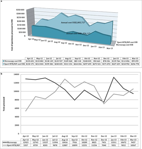
(a) Total costs for Xpert MTB/RIF and microscopy for 10 intervention laboratories for the financial year 2012/2013 ($US2013). (b) Figures for Xpert MTB/RIF and microscopy tests processed for 10 intervention laboratories for the financial year 2012/2013

The breakdown of total costs for Xpert MTB/RIF by input during each observation is presented in Table SIII. In the intervention laboratories, the proportion of total costs attributed to reagents and chemicals was on average 62% for observation 1 and 64% for observation 2. In the control laboratories, the cost for reagents and chemicals was only 24% in observation 2 (post‐Xpert MTB/RIF implementation) on average. Labour costs during the first and second observations accounted for 8% and 7%, respectively, at the intervention laboratories and 14% in the control laboratories for the second observation on average. Above laboratory costs account for 6% for the intervention and 7% for the control laboratories on average.

3.3. Unit costs

Bottom‐up and top‐down laboratory unit costs for Xpert MTB/RIF and microscopy are displayed in Tables 2 and 3, respectively. For Xpert MTB/RIF, the mean bottom‐up cost per test processed was $US16.9 (standard deviation (SD), $US6.1) in comparison with the mean top‐down cost of $US33.5 (SD, $US32.0). The mean bottom‐up unit costs were the same for observation 1 $US14.6 (SD, $US2.0) and 2 $US14.6 (SD, $US1.8) (in intervention laboratories), whereas the top‐down first observation unit cost was $US28.4 (SD, $US28.0) (in intervention laboratories) and the second observation measured a $US19.7 (SD, $US3.5) top‐down unit cost. During the start‐up stages of implementation, the mean bottom‐up unit cost of Xpert MTB/RIF in control sites was $US24.3 (SD, $US9.2) per test compared with a mean top‐down measurement of $US68.4 (SD, $US45.5).

Table 2.

Unit costs Xpert MTB/RIF: top‐down and bottom‐up costs per test processed by input type, study arm and observation ($US2013)

	Start‐up stages of implementation (~3 months of implementationa)		Early stages of implementation (~3–6 months of implementationa)		Medium term stages of implementation (~12 months of implementationa)
Time period	Control (observation 2)		Intervention (observation 1)		Intervention (observation 2)
Top down‐method	n = 5		n = 10		n = 9
	Mean	Range	Mean	Range	Mean	Range
Overheads	$0.3	($0.1; $0.6)	$3.6	($0.2; $29.4)	$0.7	($0.2; $1.7)
Transport	$0.5	($0.1; $1.0)	$0.8	($0.1; $2.9)	$0.9	($0.1; $2.9)
Building space	$0.3	($0.1; $1.2)	$1.2	($0.2; $6.4)	$0.7	($0.2; $2.1)
Equipment	$35.2	($0.6; $76.9)	$1.3	($1.0; $1.7)	$1.6	($0.9; $3.4)
Staff	$10.0	($2.2; $20.5)	$2.7	($0.5; $13.5)	$1.5	($0.1; $2.3)
Reagents and chemicals	$10.9	($9.8; $13.8)	$15.3	($10.3; $39.7)	$12.5	($9.7; $17.4)
Calibration	$1.9	($0.4; $4.1)	$0.1	($0.1; $0.7)	$0.1	($0.1; $0.1)
Training Xpert MTB/RIF specific	$5.8	($1.1; $14.1)	$0.5	($0.2; $2.1)	$0.2	($0.2; $0.5)
Consumables	$0.3	($0.1; $0.4)	$1.5	($0.0; $12.4)	$0.3	($0.0; $1.3)
Above service‐level costs Xpert MTB/RIF	$3.2	($0.1; $11.0)	$1.4	($0.7; $3.6)	$1.2	($0.7; $3.1)
Mean unit cost for each Xpert MTB/RIF observation	$68.4 (SD, $45.5)		$28.4 (SD, $28.0)		$19.7 (SD, $3.5)
Mean top down unit cost for Xpert MTB/RIF	$33.5 (SD, $32.0)
Bottom‐up method	n = 5		n = 10		n = 6
	Mean	Range	Mean	Range	Mean	Range
Overheads	$0.3	($0.0; $1.0)	$0.4	($0.1; $0.9)	$0.3	($0.1; $0.6)
Transport	$0.4	($0.1; $1.0)	$0.8	($0.1; $2.9)	$1.1	($0.1; $2.9)
Building space	$0.2	($0.1; $0.5)	$0.2	($0.0; $0.4)	$0.2	($0.0; $0.8)
Equipment	$1.6	($0.2; $3.3)	$0.5	($0.0; $0.9)	$0.8	($0.3; $1.6)
Staff	$1.0	($0.3; $1.7)	$0.9	($0.1; $4.1)	$0.7	($0.1; $1.4)
Reagents and chemicals	$9.7	($9.7; $9.7)	$9.7	($9.7; $9.7)	$9.7	($9.7; $9.7)
Calibration	$1.9	($0.4; $4.1)	$0.1	($0.1; $0.7)	$0.1	($0.1; $0.1)
Training Xpert MTB/RIF specific	$5.8	($1.1; $14.1)	$0.5	($0.2; $2.1)	$0.2	($0.2; $0.3)
Consumables	$0.2	($0.1; $0.3)	$0.1	($0.0; $0.3)	$0.1	($0.0; $0.4)
Above service‐level costs Xpert MTB/RIF	$3.2	($0.1; $11.0)	$1.4	($0.7; $3.6)	$1.4	($0.7; $3.1)
Mean unit cost for each Xpert MTB/RIF observation	$24.3 (SD, $9.2)		$14.6 (SD, $2.0)		$14.6 (SD, $1.8)
Mean bottom‐up unit cost for Xpert MTB/RIF	$16.9 (SD, $6.1)

^aAfter the last laboratory implemented Xpert MTB/RIF.

Table 3.

Unit costs microscopy: top‐down and bottom‐up costs per test processed by input type, study arm and observation ($US2013)

	Control				Intervention
Time period	Observation 1		Observation 2		Observation 1		Observation 2
Top‐down inputs	n = 9		n = 9		n = 9		n = 9
	Mean	Range	Mean	Range	Mean	Range	Mean	Range
Overheads	$0.6	($0.1; $1.3)	$0.6	($0.1; $1.3)	$1.2	($0.3; $2.8)	$1.2	($0.3; $2.8)
Transport	$0.7	($0.1; $2.1)	$0.7	($0.1; $2.1)	$0.9	($0.1; $2.9)	$0.9	($0.1; $2.9)
Building space	$0.6	($0.0; $1.5)	$0.8	($0.1; $1.5)	$1.1	($0.2; $4.4)	$1.0	($0.2; $4.4)
Equipment	$0.3	($0.1; $0.8)	$0.3	($0.0; $0.8)	$0.7	($0.2; $1.4)	$0.7	($0.2; $1.4)
Staff	$1.1	($0.4; $1.9)	$1.1	($0.4; $1.7)	$1.7	($0.5; $3.2)	$1.6	($0.3; $3.1)
Reagents and chemicals	$1.0	($0.1; $4.2)	$1.0	($0.1; $4.2)	$2.6	($0.3; $7.8)	$2.5	($0.1; $7.8)
Consumables	$0.3	($0.1; $0.4)	$0.3	($0.1; $0.9)	$0.3	($0.0; $1.3)	$0.3	($0.0; $1.3)
Above service‐level costs microscopy	$1.9	($0.7; $4.0)	$1.8	($0.6; $3.8)	$2.1	($0.4; $3.4)	$2.1	($0.4; $3.3)
Mean unit cost for each microscopy observation	$6.4 (SD, $2.0)		$6.8 (SD, $1.9)		$10.6 (SD, $3.9)		$10.4 (SD, $4.0)
Mean top down unit cost for microscopy	$8.5 (SD, $3.6)
Bottom‐up inputs	n = 9		n = 5		n = 8		n = 6
	Mean	Range	Mean	Range	Mean	Range	Mean	Range
Overheads	$0.2	($0.0; $0.5)	$0.1	($0.0; $0.3)	$0.7	($0.0; $1.9)	$0.5	($0.0; $1.9)
Transport	$0.7	($0.1; $2.1)	$0.9	($0.1; $2.1)	$0.9	($0.1; $2.9)	$1.1	($0.1; $2.9)
Building space	$0.6	($0.0; $3.6)	$0.4	($0.2; $0.6)	$0.8	($0.1; $4.5)	$0.9	($0.0; $4.5)
Equipment	$0.3	($0.1; $0.6)	$0.1	($0.1; $0.3)	$0.3	($0.1; $0.5)	$0.2	($0.1; $0.4)
Staff	$0.4	($0.1; $1.2)	$0.3	($0.2; $0.5)	$1.1	($0.1; $4.4)	$0.6	($0.2; $1.3)
Reagents and chemicals	$1.7	($0.4; $5.0)	$1.0	($0.2; $1.6)	$0.5	($0.1; $1.2)	$0.8	($0.1; $2.9)
Consumables	$0.4	($0.2; $0.9)	$0.5	($0.1; $0.9)	$0.4	($0.2; $0.8)	$0.3	($0.1; $0.7)
Above service‐level costs microscopy	$1.9	($0.7; $4.0)	$2.2	($1.5; $3.8)	$2.0	($0.4; $3.4)	$2.2	($0.4; $3.3)
Mean unit cost for each microscopy observation	$6.2 (SD, $1.7)		$5.5 (SD, $1.9)		$6.6 (SD, $3.5)		$6.7 (SD, $3.5)
Mean bottom up unit cost for microscopy	$6.3 (SD, $2.8)

A paired t‐test was performed to determine if the two methods (top‐down and bottom‐up) produced statistically different results. There were a total of 21 observations with complete data for top‐down and bottom‐up unit costs (n = 21), and these were used in the paired t‐test (Table SVI). A 95% confidence interval about the mean showed a significant difference (0 did not fall in the range 5.36 and 31.88, leading us to reject the null hypothesis that there is no difference between the two observation means). The mean (mean = 18.62; SD = 29.12; n = 21) was significantly greater than zero, and the two‐tail p = 0.008 provides evidence that the methods are notably different.

Table 4 presents the costs estimated at the reference laboratory. The mean bottom‐up and top‐down costs for each of the tests, respectively, were: microscopy $US3.6 and $US8.2; MTBDRplus $US20.3 and $US30.6; MGIT culture $US12.9 and $US16.1; and drug susceptibility testing for streptomycin, isoniazid, rifampin and ethambutol (DST MGIT SIRE) $US25.1 and $US53.7. These unit costs all include above laboratory costs. Table SIV presents our estimates of incremental costs using two methods. We estimate an average incremental cost of $US17.7 (top‐down) and $US14.7 (bottom‐up) for Xpert MTB/RIF. We present the ordinary least squares regression analysis in Figure 2. We find that scale, and by this we mean an increase in the number of specimens requiring processing and those being processed, is a strong determinant of both bottom‐up and top‐down costs with a correlation coefficient of 0.66 and 0.79, respectively, (p < 0.001).

Table 4.

Top‐down and bottom‐up unit costs for reference laboratory tests by input type, study arm and observation ($US2013)

	MTBDRplus	Fluorescence smear microscopy	MGIT Culture	DST MGIT SIRE
Laboratory name	Lab 21
Annual number of tests (for financial year 2012/2013)	18 394	73 115	126 936	3914
Unit cost per specimen processed (bottom up) $US with above service‐level costs	$20.3	$3.6	$12.9	$25.1
Unit cost per specimen processed (top down) $US with above service‐level costs	$30.6	$8.2	$16.1	$53.7

Figure 2.

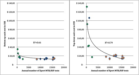
Bottom‐up and top‐down unit costs for Xpert MTB/RIF for intervention laboratories observations 1 (blue) and 2 (orange), and control laboratories (green) ($US2013) versus annual number of tests processed

4. Discussion

Using a mixed methods approach to costing, the XTEND pragmatic trial enabled us to assess and understand the costs of rolling out Xpert MTB/RIF under routine ‘real‐world’ conditions in South Africa (Churchyard, 2011). The difference between paired bottom‐up and top‐down unit costs for the laboratories were statistically significant. Our findings using the bottom‐up approach are broadly in line with previous trial‐based estimates conducted using a primarily bottom‐up method. Before the 40% price reduction in Xpert MTB/RIF cartridge costs in 2012, Vassall et al. (2011a, 2011b) estimated the cost of Xpert MTB/RIF processing through measured observation to be $US25.9 per test in South Africa. Including recent cartridge price reductions, this unit cost (equivalent to $US19.0 when the price difference is subtracted) is slightly higher than the bottom‐up cost we calculated of $US16.9 using the bottom‐up method in a routine setting and suggests that the bottom‐up methods used to cost tests during demonstration and clinical trial sites were somewhat robust to changes in ‘real‐world’ implementation in South Africa.

However, our top‐down costs differ from previous estimates. Although some of this difference may reflect some inaccuracy in allocating resources, given that most of the laboratories were performing a limited range of activities, the substantial difference in our top‐down and bottom‐up unit cost estimates also suggests a ‘real‐world’ efficiency gap. The fact that this difference may be due to efficiency rather than measurement error is reflected in the fact that the top‐down costs of Xpert MTB/RIF using the same measurement approach reduced substantially over time during roll‐out, from $US28.4 to $US19.7 in the intervention sites across the two observations, suggesting improvements in the utilisation of fixed resources during scale‐up. Our results on the relationship between cost and scale support this finding. Menzies et al. (2012a, 2012b) argue that an inverse relationship between volume and cost may be attributed to economies of scale as well as experience of those processing. The process study (Supporting Information and Table SV), using observation and discussion undertaken with laboratory staff, suggests that during roll‐out, processes and practices changed suggesting ‘learning by doing’ and poorly performing sites closed down. This learning process relates to the adaptation of the new technology within the local setting (Gilson and Schneider, 2010). It is, however, important to note that during the time that this study took place, there were substantial resource constraints on the laboratory system in South Africa, which had bearing on the closure of less efficient and lower workload settings (Treatment action campaign, 2014; Health Systems Trust, 2012). Interestingly, we find economies of scale when we use both bottom‐up and top‐down costing methods. This suggests that both resource under utilisation and the efficiency of processes become more efficient as volumes increase.

Our analysis of incremental costs suggests that the Xpert MTB/RIF did not place any substantial incremental burden on the fixed capacity of the South African laboratory system (NHLS) (Vassall et al., 2011a; Vassall et al., 2011b). Our method to assess incremental cost is simple but is complemented by our process evaluation, which finds no increase was required in the total levels of building and human resources during the period of roll‐out. We found that, although the focus of effort shifted in intervention laboratories, overall levels of staffing remained the same as for microscopy and that any increased infrastructure requirements were absorbed with longer opening hours.

It is unlikely that the specific findings above are generalizable or can be applied across settings and different new technology types. In our case, our measurement of incremental costs, due to the excess capacity in fixed costs and the scale effect, did not substantially impact our previous conclusions on cost‐effectiveness using bottom‐up measures at a smaller scale. Similar studies examining costs of HIV prevention and/or treatment have shown similar patterns of cost reductions over time and by scale (Lépine et al., 2015; Tagar et al., 2014; Menzies et al., 2012b). However, South Africa has a well‐developed laboratory system, and other technologies have markedly different resource profiles. Improvements over time in efficiency will also be highly dependent on programme and site management and the volumes of tests at each site required to ensure high coverage. Therefore, analysts should not presume that in all cases, initial bottom‐up costs are accurate predictors of unit costs at scale when estimating cost‐effectiveness.

Our study also highlights that care needs to be taken regarding when to measure costs. Total costs fluctuate according to seasonal trends in TB rates and testing practices (Koh et al., 2013). Some of the fluctuation was also caused by stock‐out of laboratory supplies during the roll‐out process. Xpert MTB/RIF cartridge stock‐outs occurred in July, September, October 2012 and February 2013 because of insufficient supply from the stockists (Molapo, 2013). Laboratories often compensated for this by borrowing stock from other laboratories.

Our findings earlier are subject to certain limitations. The percentage of laboratories that was not observed for all the planned observations may have biased the findings in terms of measures of efficiency. Our sample size, although large for a costing study, was too small for performing more sophisticated econometrics to analyse cost drivers. Although it allowed for the scope of methods used, including robust economies of scale and statistical analysis of costs using the two different methods. Care should be taken when generalising our findings to other settings (as described earlier). Our findings in this setting are highly dependent on the proportion of fixed costs and the extent and characteristics of inefficiency within the South African laboratory systems. Top‐down and bottom‐up methods may therefore align better in other settings. More studies are needed to examine this research gap, and we recommend further testing in other areas prior to the full acceptance of the use of these dual methodologies.

Current guidance on how to incorporate efficiency into cost estimation is often broad, suggesting assumptions (such as applying 80% capacity usage) acknowledging that in practice this is likely to vary by healthcare setting (Drummond et al., 1997). New tools, such as the OneHealth Tool (which is publically available for download), are being developed that allow the improved estimation of capacity across a health system (Futures Institute, 2014) but as yet cannot be applied to specific new technologies. Given the range of costing estimates found using different approaches, we recommend that when making country‐specific estimates of incremental costs for cost‐effectiveness or budget impact purposes to use the dual approach suggested here. As this may not always be feasible, at the very least, analysts should more carefully present, which costs were measured using the different approaches.

Bottom‐up costing methods are more feasible where procedures are frequently performed and/or detailed resource use data are available, for instance, with patient‐level resource use (Mercier and Naro, 2014; Wordsworth et al., 2005). They can pose a logistical challenge, however, where the procedures are performed infrequently and observation may also bias results by impacting the behaviour of those conducting the procedure. In comparison, the top‐down method included here required considerable engagement and participation by the study sites in terms of access to expenditure data and willingness to fill in data collection instruments such as timesheets (Wordsworth et al., 2005). This level of engagement may only be feasible where funding is sufficient and the time frame allows for agreements to be made early on during a costing study. A particular issue is that expenditure data for top‐down costing is in centralised systems, which may not be accessible at study sites and can take considerable time and effort to access and apportion. Hendriks et al. (2014) provide an illustrative guide to collecting top‐down cost data when expenditure data are difficult to collect. Nevertheless, once that engagement is established and access provided, we found that using both methods was not substantially more time consuming per site.

Moreover, the two costing methods provided complementary insight for NHLS managers in South Africa and have several policy and practice implications beyond economic evaluation, which is contrary to the interpretation of using both practices by Mercier and Naro (2014) who found the lack of agreement between the two methods disagreeable. Commonly, budget setting and negotiations in South Africa use a method of bottom‐up ingredients costing. But in practice, real expenditure (as captured in top‐down methods) exceeds these funds, creating substantial budgetary pressure. These two measurements of costs allow for a more informed discussion of the budget during and post‐scale‐up. Such discussions should also include an assessment of feasible efficiency improvements. Moreover, the comparison between these costs from specific sites allow the NHLS to identify areas and practices that require further process and efficiency improvement in specific sites during the final stages of roll‐out.

Finally, the sample size of our study was considerably larger than is common in costing studies of new technologies at early stages of global roll‐out generally, which is rarely feasible given the scarce funding for such studies. However, this sample size enabled some assessment of economies of scale that may be useful in promoting discussion on Xpert MTB/RIF placement in other settings. In addition, it provides information for policy makers and planners to provide adequate budgets for settings with low‐density populations (as is common in many LMIC settings). More analysis is required to better understand the trade‐off between ensuring thorough site‐level data collection versus increasing sample size.

5. Conclusion

This study provides an example of a pragmatic, but comprehensive, approach to measuring the costs of new technologies during their roll‐out, which can be incorporated into economic evaluations and budget impact estimates in LMIC settings. The clarity gained from being explicit about bottom‐up and top‐down approaches, together with a moderate sample size, process study, observation and discussion with laboratory staff, can support policy makers and planners to make more accurate estimates of the resource requirements of the scale‐up of new technologies in settings where resources are extremely scarce.

Conflicts of Interest

We declare no conflicts of interest.

Supporting information

Supporting info item

Cunnama, L. , Sinanovic, E. , Ramma, L. , Foster, N. , Berrie, L. , Stevens, W. , Molapo, S. , Marokane, P. , McCarthy, K. , Churchyard, G. , and Vassall, A. (2016) Using Top‐down and Bottom‐up Costing Approaches in LMICs: The Case for Using Both to Assess the Incremental Costs of New Technologies at Scale. Health Econ., 25: 53–66. doi: 10.1002/hec.3295.

References

- Adam T et al. 2008. Capacity utilization and the cost of primary care visits: Implications for the costs of scaling up health interventions. Cost effectiveness and resource allocation 6: 1–9. Available at: http://www.pubmedcentral.nih.gov/articlerender.fcgi?artid=2628647&tool=pmcentrez&rendertype=abstract [Accessed September 26, 2014]. [DOI] [PMC free article] [PubMed] [Google Scholar]
- Batura N et al. 2014. Collecting and analysing cost data for complex public health trials: reflections on practice. Global Health Action 7: 1–9. [DOI] [PMC free article] [PubMed] [Google Scholar]
- Chapko MK et al. 2009. Equivalence of two healthcare costing methods: Bottom‐up and top‐down. Health Economics 18: 1188–1201. [DOI] [PubMed] [Google Scholar]
- Churchyard G. 2014. Effect of Xpert MTB/RIF on early mortality in adults with suspected TB: a pragmatic randomized trial In 21st Conference on Retroviruses and Opportunistic Infections, 3–6 March 2014, Oral Abstract 95. Boston: Available at: http://www.croiwebcasts.org/console/player/22178 [Accessed October 27, 2015]. [Google Scholar]
- Churchyard G, 2011. “Xpert for TB: Evaluating a new diagnostic” (EXTEND) trial, Johannesburg.
- Churchyard GJ et al. 2015. Xpert MTB/RIF versus sputum microscopy as the initial diagnostic test for tuberculosis: a cluster‐randomised trial embedded in South African roll‐out of Xpert MTB/RIF. Lancet Global Health 3: 450–457. Available at: http://ac.els‐cdn.com/S2214109X1500100X/1‐s2.0‐S2214109X1500100X‐main.pdf?_tid=a91481a4‐400e‐11e5‐b663‐00000aab0f6c&acdnat=1439286921_17664dd8fc375f35c6fa79a0cc830651 [Accessed October 27, 2015]. [DOI] [PubMed] [Google Scholar]
- Conteh L, Walker D. 2004. Cost and unit cost calculations using step‐down accounting. Health Policy and Planning 19(2): 127–135. Available at: http://www.heapol.oupjournals.org/cgi/doi/10.1093/heapol/czh015 [Accessed March 24, 2014]. [DOI] [PubMed] [Google Scholar]
- Drummond M et al. 1997. Methods for the Economic Evaluation of Health Care Programmes(2nd edn), Oxford University Press: New York, United States of America. [Google Scholar]
- Flessa S et al. 2011. Basing care reforms on evidence: the Kenya health sector costing model. BMC Health Services Research 11(128): 1–15. Available at: http://www.pubmedcentral.nih.gov/articlerender.fcgi?artid=3129293&tool=pmcentrez&rendertype=abstract [Accessed October 27, 2015]. [DOI] [PMC free article] [PubMed] [Google Scholar]
- Futures Institute . 2014. OneHealth Tool. Available at: http://www.futuresinstitute.org/onehealth.aspx [Accessed October 27, 2015].
- Gilson L, Schneider H. 2010. Commentary: managing scaling up: What are the key issues? Health Policy and Planning 25(2): 97–98. [DOI] [PubMed] [Google Scholar]
- Health Systems Trust . 2012. National Health Laboratory Service still struggling with tardy provincial payments.
- Hendriks ME et al. 2014. Step‐by‐step guideline for disease‐specific costing studies in low‐and middle‐income countries: a mixed methodology. Global Health Action 7: 1–10. [DOI] [PMC free article] [PubMed] [Google Scholar]
- Koh GCKW et al. 2013. Tuberculosis Incidence Correlates with Sunshine: an Ecological 28‐Year Time Series Study. PLoS ONE 8(3): 1–5. [DOI] [PMC free article] [PubMed] [Google Scholar]
- Lépine A et al. 2015. Estimating unbiased economies of scale of HIV prevention projects: a case study of Avahan. Social Science & Medicine 131: 164–72. Available at: http://www.ncbi.nlm.nih.gov/pubmed/25779621 [Accessed October 27, 2015]. [DOI] [PubMed] [Google Scholar]
- Menzies N, Cohen T et al. 2012a. Population health impact and cost‐effectiveness of tuberculosis diagnosis with Xpert MTB/RIF: a dynamic simulation and economic evaluation. PLoS Medicine 9(11): 1–17. Available at: http://www.pubmedcentral.nih.gov/articlerender.fcgi?artid=3502465&tool=pmcentrez&rendertype=abstract [Accessed March 24, 2014]. [DOI] [PMC free article] [PubMed] [Google Scholar]
- Menzies N, Berruti A, Blandford J. 2012b. The Determinants of HIV Treatment Costs in Resource Limited Settings. PLoS ONE 7(11): 1–19. [DOI] [PMC free article] [PubMed] [Google Scholar]
- Mercier G, Naro G. 2014. Costing hospital surgery services: The method matters. PLoS One 9(5): 1–7. Available at: http://www.pubmedcentral.nih.gov/articlerender.fcgi?artid=4016301&tool=pmcentrez&rendertype=abstract [Accessed November 6, 2014]. [DOI] [PMC free article] [PubMed] [Google Scholar]
- Molapo S. 2013. E‐mail to Lucy Cunnama (nee Shillington) 10 September.
- National Department of Health . 2014. National Tuberculosis Management Guidelines, Pretoria, South Africa. Available at: http://www.sahivsoc.org/upload/documents/NTCP_Adult_TBGuidelines 27.5.2014.pdf [Accessed October 27, 2015].
- National Health Laboratory Service . 2013. GeneXpert MTB/RIF Progress report, Available at: http://www.nhls.ac.za/assets/files/GeneXpert Progress Report August 2013_Final.pdf [Accessed October 27, 2015].
- Simoens S. 2009. Health economic assessment: a methodological primer. International Journal of Environmental Research and Public Health 6(12): 2950–66. Available at: http://www.pubmedcentral.nih.gov/articlerender.fcgi?artid=2800325&tool=pmcentrez&rendertype=abstract [Accessed November 10, 2014]. [DOI] [PMC free article] [PubMed] [Google Scholar]
- Steingart K et al. 2014. Xpert® MTB/RIF assay for pulmonary tuberculosis and rifampicin resistance in adults. Cochrane Database Systematic Review, Issue(1): 1–166. Available at: http://onlinelibrary.wiley.com/doi/10.1002/14651858.CD009593.pub3/pdf/standard [Accessed March 18, 2014]. [DOI] [PMC free article] [PubMed] [Google Scholar]
- Tagar E et al. 2014. Multi‐Country Analysis of Treatment Costs for HIV/AIDS (MATCH): Facility‐Level ART Unit Cost Analysis in Ethiopia, Malawi, Rwanda, South Africa and Zambia. PLoS Medicine 9(11): 1–9. [DOI] [PMC free article] [PubMed] [Google Scholar]
- Treatment action campaign . 2014. NHLS oversight in crisis ‐ patients pay the price. Available at: http://www.tac.org.za/news/nhls‐oversight‐crisis‐patients‐pay‐price [Accessed August 12, 2015].
- UNAIDS . 2011. Manual for costing HIV facilities and services. Available at: http://www.unaids.org/en/media/unaids/contentassets/documents/document/2011/20110523_manual_costing_HIV_facilities_en.pdf [Accessed October 27, 2015].
- Vassall, A. , Sinanovic, E et al. 2011a. Evaluating the cost of scaling up Xpert MTB/RIF in the investigation of tuberculosis in South Africa, Johannesburg.
- Vassall, A. , van Kampen, S et al. 2011b. Rapid diagnosis of tuberculosis with the Xpert MTB/RIF assay in high burden countries: a cost‐effectiveness analysis. D. Wilson, ed. PLoS Medicine 8(11): 1–14. Available at: http://dx.plos.org/10.1371/journal.pmed.1001120 [Accessed March 22, 2014]. [DOI] [PMC free article] [PubMed] [Google Scholar]
- Wordsworth S et al. 2005. Collecting unit cost data in multicentre studies: Creating comparable methods. The European Journal of Health Economics 50(1): 38–44. Available at: http://www.ncbi.nlm.nih.gov/pubmed/15772871 [Accessed November 20, 2014]. [DOI] [PubMed] [Google Scholar]
- World Health Organisation , 2010. Media centre: WHO endorses new rapid tuberculosis test. Available at: http://www.who.int/mediacentre/news/releases/2010/tb_test_20101208/en/ [Accessed October 27, 2015].
- World Health Organization , 2013. Automated real‐time nucleic acid amplification technology for rapid and simultaneous detection of tuberculosis and rifampicin resistance: Xpert MTB/RIF assay for the diagnosis of pulmonary and extra‐pulmonary TB in adults and children. Policy update, Geneva, Switzerland. Available at: http://apps.who.int/iris/bitstream/10665/112472/1/9789241506335_eng.pdf [Accessed October 27, 2015]. [PubMed]
- World Health Organization , 2014. Global Tuberculosis Report 2014, Geneva, Switzerland. Available at: http://www.who.int/tb/publications/global_report/en/ [Accessed October 27, 2015].
- World Health Organization , 2002. Guidelines for cost and cost‐effectiveness analysis of tuberculosis control, Available at: http://whqlibdoc.who.int/hq/2002/WHO_CDS_TB_2002.305a.pdf?ua=1 [Accessed October 27, 2015].
Associated Data
This section collects any data citations, data availability statements, or supplementary materials included in this article.
Supplementary Materials