Estimating 3D tilt from local image cues in natural scenes

Abstract

Estimating three-dimensional (3D) surface orientation (slant and tilt) is an important first step toward estimating 3D shape. Here, we examine how three local image cues from the same location (disparity gradient, luminance gradient, and dominant texture orientation) should be combined to estimate 3D tilt in natural scenes. We collected a database of natural stereoscopic images with precisely co-registered range images that provide the ground-truth distance at each pixel location. We then analyzed the relationship between ground-truth tilt and image cue values. Our analysis is free of assumptions about the joint probability distributions and yields the Bayes optimal estimates of tilt, given the cue values. Rich results emerge: (a) typical tilt estimates are only moderately accurate and strongly influenced by the cardinal bias in the prior probability distribution; (b) when cue values are similar, or when slant is greater than 40°, estimates are substantially more accurate; (c) when luminance and texture cues agree, they often veto the disparity cue, and when they disagree, they have little effect; and (d) simplifying assumptions common in the cue combination literature is often justified for estimating tilt in natural scenes. The fact that tilt estimates are typically not very accurate is consistent with subjective impressions from viewing small patches of natural scene. The fact that estimates are substantially more accurate for a subset of image locations is also consistent with subjective impressions and with the hypothesis that perceived surface orientation, at more global scales, is achieved by interpolation or extrapolation from estimates at key locations.

Introduction

One of the most fundamental and difficult tasks for the visual system is to estimate three-dimensional (3D) surface shape from the pair of two-dimensional images formed by the left and right eyes. To estimate surface shape, the visual system makes use of many different sources of information (cues), including binocular disparity (Backus & Banks, 1999; Knill, 2007; Ogle, 1952), texture (Blake, Bulthoff, & Sheinberg, 1993; Knill, 1998a, 1998b), shading and lighting (Fleming, Torralba, & Adelson, 2004; Mamassian, Knill, & Kersten, 1998), surface boundary shape (Burge, Fowlkes, & Banks, 2010a; Palmer & Ghose, 2008; Peterson & Gibson, 1993), and motion parallax (Landy, Maloney, Johnston, & Young, 1995). Each of these cues has received a great deal of attention in the psychophysical, computational, and neuroscience literature. As a whole, these studies have demonstrated that these cues provide useful information for estimating surface shape but also that none of the cues alone is sufficient to approach human performance in natural scenes. Thus, there has been much interest recently in how the visual system combines different cues to obtain more precise and more accurate estimates.

An effective paradigm has been to create synthetic stimuli in which two different cues can be manipulated independently. Human estimation or discrimination performance is then measured for each cue separately and in combination (Burge, Girshick, & Banks, 2010b; Gepshtein, Burge, Ernst, & Banks, 2005; Hillis, Ernst, Banks, & Landy, 2002; Hillis, Watt, Landy, & Banks, 2004; Knill, 1998b; Landy et al., 1995). In a number of cases, it has been found that the visual system combines cues in an optimal fashion, under the assumption that estimates from the cues are uncorrelated and Gaussian distributed (Burge et al., 2010b; Hillis et al., 2002, 2004). The optimal combined estimate (given uncorrelated Gaussian distributions) is the weighted sum of the two estimates (linear cue combination) in which the weight on each estimate is its relative reliability (inverse of the variance; Alais & Burr, 2004; Clark & Yuille, 1990; Ernst & Banks, 2002). For example, if the cues are equally reliable, then the reliability of the estimate would increase by a factor of two over that of each cue individually. On the other hand, if one of the cues is much less reliable than the other, there will be little improvement in reliability, even if the cues are combined optimally. Worse yet, if the cues are combined under a mistaken assumption that they are equally reliable, performance can easily be worse than just using the better of the two cues. A particularly important fact in this context is that the different cues often vary in their relative reliability across different locations in natural images. Thus, an effective cue combination requires taking into account the local relative reliability.

In the computational literature, there are many proposed algorithms for estimating surface shape from a single cue (“shape from X”; Malik & Rosenholtz, 1994; Watanabe & Nayar, 1998); however, there have been few attempts to consider multiple cues (Saxena, Schulte, & Ng, 2007) and few attempts to directly analyze the statistics of different cues in natural scenes (Potetz & Lee, 2003; Saxena, Chung, & Ng, 2008).

Making measurements in natural scenes is important because (a) the estimates from different cues may not be statistically independent and/or may not be Gaussian distributed in natural scenes, (b) the relative reliabilities of the different cues in natural scenes are unknown, and (c) one would expect the cue combination rules used by the visual system to be optimized for the statistical structure of natural scenes.

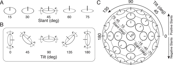
The most local measure of 3D surface shape is the 3D orientation of the tangent plane at a point on the surface. Presumably, the visual system integrates the local measurements of 3D surface orientation into a representation of surface shape. The 3D surface orientation can be decomposed into two parts: the surface slant and the surface tilt (Figure 1). Slant is the amount a surface is rotated out of the reference (e.g., frontoparallel) plane (Figure 1A). Tilt is the direction in the reference plane that the distance to the surface is changing most rapidly, the so-called “direction of slant” (Stevens, 1983). Tilt is equivalently defined as the orientation of the surface normal's projection in the reference plane (Figure 1B). Note that the tilt angle is always orthogonal to the axis in the reference plane about which the surface is rotated.

Figure 1.

Definition of slant and tilt. (A) Slant is the angle of rotation out of the reference plane (e.g., fronto-parallel plane). (B) Tilt is the orientation of the surface normal projected into the reference plane. It is always orthogonal to the axis about which the surface is rotated. (C) Slant and tilt together define a unique 3D surface orientation. The joint slant-tilt vector defines a point on the surface of a unit sphere. Different conventions exist for representing surface orientation. In this plot, we show tilts on [0 180) and slants on [−90 90). Other conventions represent tilt on [0 360) and slants on [0 90).

Here we describe a statistical analysis of cues to local 3D orientation in natural scenes. This article focuses on tilt, although we also report some results for slant. There are many potential cues to local tilt that could be examined given our database of registered ground-truth range images and stereo-camera images. We consider three cues: the orientation of the local gradient of binocular disparity, the orientation of the local gradient of luminance, and the dominant orientation (major axis) of the local texture. These were picked primarily for their simplicity, historical precedence, and their plausibility given known processing in the early visual system. In a follow-up analysis, we also evaluate the usefulness of several local auxiliary cues: mean absolute disparity (vergence demand), mean luminance, and RMS contrast, which are also simple and plausible given known processing in the early visual system.

We analyze how to estimate unsigned tilt (Figure 1) given the measured cue values. This makes our analysis equivalent to estimating the orientation of the axis about which depth is changing most rapidly. Even though 3D surface tilt contributes strongly to the results presented here, our analysis does not distinguish between the tilt of surfaces belonging to individual objects and the tilt (i.e., orientation) of depth discontinuities (object boundaries). We therefore emphasize that our analysis is best thought of as 3D tilt rather than 3D surface tilt estimation. To carry out the analysis, we first obtained a database of high-resolution stereo-camera images, along with co-registered high-resolution range images. From the range images, we obtained ground-truth measurements of the local tilt at each scene location. From the pair of camera images, we measured the local image cues at each location where the ground-truth tilt was measured.

We analyze the range and image data in two ways: in a conditional-means framework and in a linear-summation framework. The conditional-means framework has the advantage that it provides the Bayes optimal estimates (given a squared error cost function) for the individual cues, pairs of cues, or all three cues together, without making assumptions about statistical independence or about the form of the joint probability distribution (which is four-dimensional: range, disparity, texture, and luminance). This assumption-free analysis is useful because it can provide new insight into how the visual system should combine these cues, given the statistical structure of natural scenes, and because the computations implicit in the optimal estimates can suggest principled and testable hypotheses for cue combination in the visual system. However, its disadvantage is that the data requirements make it impossible to consider more than three variables (cues) at a time. The linear-summation framework has the advantage that it is possible to analyze the potential value/role of additional auxiliary cues on tilt estimation. Its disadvantage is that it may be suboptimal for two or more cues and may not exploit useful nonlinear relationships that exist between the cues in natural images.

In this study, we consider how to optimally combine image cues only at a single location. In other words, we do not consider global cues or how best to integrate image cues across space. Undoubtedly, the power the human visual system to encode the 3D structure of the environment depends in large part on effectively exploiting global cues and constraints. Nonetheless, the visual system starts with local measurements and then combines those local measurements into the global representations; the more accurate the local measurements, the more accurate the global representation. Thus, it is important to understand how cues at a single location should be combined. Also, it is possible to measure the performance of the visual system for localized stimuli taken from natural scenes, where the global cues and constraints are unavailable. Indeed, one goal of our study was to determine how local cues should be combined to estimate tilt in natural images, in order to obtain principled, testable hypotheses and predictions for human performance on localized natural stimuli.

We find that tilt estimates based on an optimal combination of cues at a single location are typically not very accurate and tend to be strongly influenced by the prior probability distribution. This result is consistent with the subjective impression from viewing small randomly selected patches of natural scenes (and with psychophysical measurements; Kim & Burge, 2016). Nonetheless, there are large subsets of image locations where the estimates are substantially more accurate (e.g., locations where the values of the cues approximately agree and locations having greater slant). This is also consistent with subjective impression and with the hypothesis that perceived surface orientation, at more global scales, is often achieved by interpolation and extrapolation from estimates at key locations.

Methods

Registered camera and range images

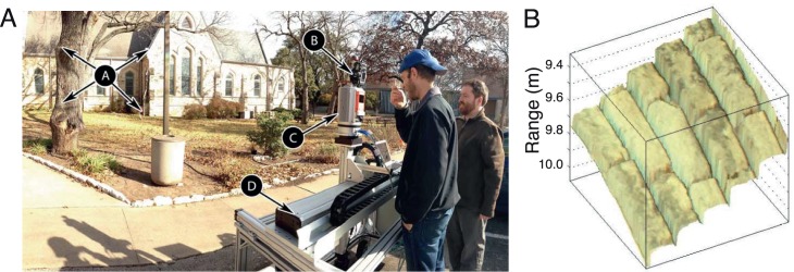
High-resolution stereo-camera and range images were obtained with a Nikon D700 digital camera mounted on a Riegl VZ-400 3D laser range scanner. The camera and laser scanner were mounted on a custom portable robotic gantry having four degrees of freedom: translation in x, y, and z and rotation about the vertical (y) axis (Figure 2A). The robotic gantry served an important function. Under normal circumstances, the fact that the camera is mounted above the range finder means that the nodal points of two instruments are not aligned, which results in missing data because of half-occlusions. Specifically, a substantial number of pixels in the camera image will have no corresponding range value, and another substantial number of pixels in the range scan will have no corresponding image value. To avoid this problem, the robotic gantry was used to align the nodal points of the camera and range scanner. The specific sequence for image capture was as follows: (a) capture the first range image, (b) translate parallel to earth vertical and perpendicular to the line of sight by 6.5 cm and capture the second range image, (c) translate vertically to align the camera nodal point to that of the second range image and capture one of the camera images, (d) translate back 6.5 cm and capture the other camera image.

Figure 2.

Registered range and camera images. (A) Camera and laser range scanner mounted on portable four-axis robotic gantry: (A) natural scene, (B) Nikon D700 DSLR camera, (C) Riegl VZ-400 3D range scanner, (D) custom robotic gantry. (B) A 200 × 200 pixel patch of a camera image of stone structure mapped onto the range image. The registration is generally within plus or minus one pixel. Note that the shadows in the camera image coincide with the mortared seams in the stone structure.

Each digital camera image was 4,284 × 2,844 pixels, with a bit depth of 14 bits per RGB color channel. Each pixel subtended about 0.02°. The camera was calibrated so that the images could be converted to eight-bit luminance images (camera spectral sensitivities are available at http://natural-scenes.cps.utexas.edu/db.shtml). The range scanner provides accurate depth measurements (±5 mm) over the range of approximately 2 m to 200 m (beam width expands 30 mm per 100 m).

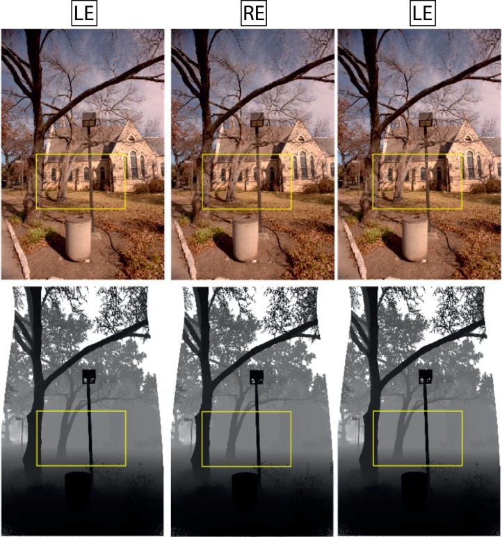
The Riegl software does not allow registration of range images with the raw 14-bit camera images. We developed custom software to register the images. Inspection of various test cases shows that we obtained very good registration (±1 pixel). The precision is illustrated in Figure 2B, which shows a 3D rendering of a small part of a camera image of a stone structure mapped onto the range image. Figure 3 shows examples of the camera and range images.

Figure 3.

Registered stereo pairs of camera images (top) and range scans (bottom). The gray scale in the bottom row indicates the range; white pixels indicate no data. Cross-fuse the left two images, or divergently fuse the right two images to see the stereo-defined depth. The yellow rectangle indicates the image regions that were used for analysis. The range data were collected with a cylindrical projection surface. The missing bits of range data in the upper right and left corners of range scans result from the geometric procedures that were required to co-register the camera image and range scans.

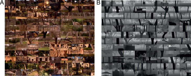
For the present study, we obtained 96 high-quality registered stereo-camera and range images from around the University of Texas campus. Images were captured from the typical eye height of a 6-ft-tall male, 66 in. above the ground. Gaze was approximately earth parallel. Fixation was at infinity. We then cropped the images to 35° × 20° of visual angle (1,920 × 1,080, yellow rectangles, Figure 3) to minimize the potential effects of camera lens distortions (e.g., barrel distortion). Thumbnails of the cropped regions from all 96 left-eye camera and range images are shown in Figure 4. This entire image set, and some additional details about the measurement system, image calibration, and registration are available at http://natural-scenes.cps.utexas.edu/db.shtml.

Figure 4.

Thumbnails of the 96 images in the data set. (A) Camera images. (B) Co-registered range images. Only the left image of each stereo-pair is shown.

Ground truth tilt and slant

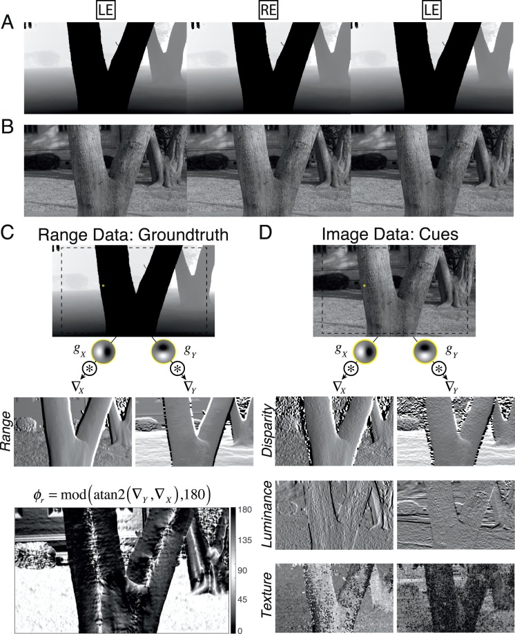
The first step of the analysis was to measure the ground-truth 3D orientation at each pixel location in the range images, for which there was no missing data in the neighborhood of the pixel. (The most common cause of missing data was scene distance beyond the limit of the range scanner, e.g., the white pixels in Figure 3, bottom row.) To obtain the ground-truth 3D orientation, we first filtered (blurred) the range image with a Gaussian kernel having a standard deviation of the 0.1° (∼five camera pixels), took the derivative in each direction, and then divided by the (local average) range to obtain a normalized range gradient vector:

where r(x,y) is the average range in the neighborhood of (x,y), with x and y in degrees of visual angle. The average range is given by the convolution of the range image with the Gaussian kernel, r(x,y) = rng(x,y) * g(x,y;σ_blur) , where g(x,y;σ_blur) is an isotropic two-dimensional Gaussian with mean zero and standard deviation σ_blur of 0.1°. For notational convenience, we leave implicit the (x,y) coordinates in the right side of Equation 1. Note that blurring the range image with a Gaussian and then taking derivatives in x and y is equivalent to convolving the range image with Gaussian derivative kernels in x and y (see Figure 5). Also note that normalizing by the range in Equation 1 is necessary so that a planar surface will be assigned the same slant independent of range; however, this normalization has no effect on the definition of tilt because the normalization term cancels out. Finally, note that this definition of ground truth tilt means that ground truth tilt depends in part on the size of the analysis neighborhood (see Discussion).

Figure 5.

Range and photographic stereo images and range and image gradients for tilt estimation. (A) Range stereo images. Light gray scales correspond to larger distances. Divergently fused the left to images, or cross-fuse the right two images. (B) Co-registered photographic stereo images. (C) Ground-truth range data, x and y components of the range gradient, and ground-truth tilts. The small yellow circle indicates the approximate size of the gradient operator (i.e., analysis window). (D) Luminance image data, and x and y components of the disparity gradient (only left eye image shown), luminance gradient, and texture gradient.

The tilt [0,360) is the inverse tangent of the ratio of the derivatives in the vertical and horizontal directions,

and the slant is the inverse tangent of the length of the gradient vector,

Note that slant is defined on an open interval [0 90) because a slant 90° surface (i.e., a depth discontinuity) projects to an infinitesimal solid angle; all of our measurements are over a solid angle with a ∼0.25° diameter.

Local image cues

The next step of the analysis was to measure the three image cues at those locations for which we were able to measure the range gradient. The first cue is based on the disparity gradient, which is defined analogously to the range gradient:

where δ(x,y) = dsp(x,y) * g(x,y;σ_blur). Again, normalizing by the (local average) disparity is necessary so that a planar surface will be assigned the same slant independent of viewing distance (but has no effect on the tilt estimate).

The disparity at each pixel location was taken to be the horizontal offset that gave the maximum normalized cross-correlation between the left and right images computed over a region the size of the Gaussian kernel (see the Appendix, Figure A2). We use local cross-correlation because this is a popular model for disparity estimation, for which there is substantial psychophysical (Banks, Gepshtein, & Landy, 2004; Tyler & Julesz, 1978) and neurophysiological (Nienborg, Bridge, Parker, & Cumming, 2004) evidence.

The disparity tilt cue is defined as the orientation of the disparity gradient:

The second cue is based on the luminance gradient, which is defined analogously:

where l(x,y) = lum(x,y) * g(x,y;σ_blur). Here we divide by the (average local) luminance so that the luminance gradient vector corresponds to the signed Weber contrasts in the horizontal and vertical directions. The luminance tilt cue is defined as the orientation of the luminance gradient:

We use the orientation of the local luminance gradient because it is a simple well-known feature extracted early in the visual system (e.g., by simple cells in primary visual cortex).

The third cue is the dominant orientation of the image texture, which we define in the Fourier domain. First, we subtract the mean luminance and multiply by (window with) the Gaussian kernel above centered on (x,y). We then take the Fourier transform of the windowed image and compute the amplitude spectrum. Finally, we use singular value decomposition to find the major (principle) axis of the amplitude spectrum (the orientation along which there is the greatest variance around the origin). We define the tilt cue as the orientation of the major axis in the Fourier domain:

where (u_x,u_y) is the unit vector defining the principle axis.

Note that unlike the tilt measure for range, disparity, and luminance, this tilt measure is ambiguous up to a rotation of ±180°; thus, the range of the tilt measure for texture is [0,180). (The ambiguity of the tilt measure is strictly true under orthogonal projection, but the differences between orthogonal and perspective projection are negligible for the small patch sizes being considered here.) We use the dominant orientation cue because it is a simple measure likely to be computed in the early visual system and because it is well known that humans are able to make fine discriminations of texture orientation (Knill & Saunders, 2003). It is a principled measure of tilt for locally isotropic textures. For example, textures composed of isotropic elements become elongated in the direction perpendicular to the direction of slant, creating a dominant orientation in the direction perpendicular to the direction of slant (Stevens, 1983). (Note that the major axis orientation in the Fourier domain corresponds to the orientation perpendicular to the dominant orientation in the space domain.) We also considered standard measures (based on local spatial frequency gradients) that do not assume isotropy, but they performed poorly on our natural images compared with the simpler dominant orientation measure (see Discussion).

Conditional means

Biological systems evolve to exploit the statistical relationships in natural scenes, and there has undoubtedly been great pressure for accurate 3D perception. Thus, it is sensible to consider how local image cues should be combined to estimate 3D tilt. If the evolutionary pressure is to make estimates that are as accurate as possible on average (with the minimum mean squared error), then it is straightforward to show that the Bayes optimal estimate is simply the mean of the posterior probability distribution conditional on the available information:

where ϕ_r is the ground-truth tilt (the latent variable) and ϕ is the observed vector of cue values [e.g., {ϕ_d,ϕ_l,ϕ_t}].

At first thought, it may seem impossible to determine the optimal—minimum mean squared error (MMSE)—estimate in the general case because of the “curse of dimensionality.” That is, the joint probability distribution p(ϕ_r,ϕ_d,ϕ_l,ϕ_t) of image cue values and ground-truth 3D tilt is four-dimensional (range, disparity, luminance, texture), and estimating it accurately would require far more data than our already quite large data set contains. However, measuring conditional means requires much less data and is practical for our size data set. The direct way to determine the conditional means is to (a) compute a running count of the number of occurrences of each unique vector of image cue values, (b) compute a running sum of the variable of interest (the unit vector in the ground truth tilt direction) for each unique vector of image cue values, and (c) compute the argument (arg) of the vector average:

where Ω(ϕ) indicates the set of ground-truth values that co-occur with a particular vector of cue values and N(ϕ) is the count of the number of occurrences of each unique vector. The circular variance of the optimal estimate (i.e., the inverse of reliability) is one minus the complex absolute value of the vector average:

These definitions of the conditional mean and variance are used because tilt and tilt cues are circular variables (see the Appendix).

The conditional means (and variances, if desired) must be computed for all possible combinations of conditioning cue values ϕ = {ϕ_d,ϕ_l,ϕ_t}. For continuous variables such as gradients, the number of possible combinations is infinite. Therefore, it is necessary to quantize the cue values. Here, we quantize each of the cue values into 64 bins, each of which is 2.8° wide. (This bin width appears to be sufficiently narrow given the smoothness of the space.) With a triplet of cue values, this quantization results in 64³ total bins, which means that ∼260,000 total conditional means must be computed. Estimating 260,000 conditional means requires a substantial amount of data. Our data set contains approximately 1 billion pixels. If the image cue triplets were uniformly distributed, each bin would have approximately 4,000 samples. In practice, we find that the minimum number of samples is 618 and the maximum 86,838. This number of samples is sufficient to reliably estimate the mean and variance for each bin.

Linear estimate combination

In the linear summation framework considered here, the combined estimate is given by

where (Φ̂_r|δ,Φ̂_r|l,Φ̂_r|t) are the estimates from the individual cues, (ρ_r|δ,ρ_r|l,ρ_r|t) are their relative reliabilities, and w₀ and ϕ₀ are constants to correct for any overall bias because the prior contributes to each of the individual estimates. In the present case, the constants are equal to zero because there is no overall bias. There are several things to note about Equation 12. First, this vector summation rule is appropriate for circular variables. Mittelstaedt (1983, 1986) was the first to show that vector summation weighted by reliability can account for human performance in cue combination experiments (Mittelstaedt, 1983, 1986). Murray and Morgenstern (2010) showed that it is near optimal under some circumstances. Second, for circular variables, using the reliabilities instead of the relative reliabilities yields the same result. Third, the linear estimate combination is different from the linear cue combination. However, for standard (not circular) variables, and the usual conditional independence and Gaussian assumptions, the linear cue combination and linear estimate combination give the same estimates (see Supplement). The advantage here of linear estimate combination is that the individual estimates (from the conditional means) are guaranteed to be optimal, independent of the shape of the individual cue posterior probability distributions and the prior probability distribution (see above). Fourth, even so, the statistical properties that are known to guarantee optimality of linear estimate combination do not hold here. Nonetheless, one can still ask how well the linear estimate combination approximates the optimal estimates.

The strength of the linear summation framework is that it requires less data and hence allows incorporation of additional auxiliary cues. Auxiliary cues can be incorporated into the individual cue estimates and their relative reliabilities (see below). Here we consider three local auxiliary cues: local mean disparity, local mean luminance, and local RMS contrast.

Results

Conditional means: Accuracy of estimates

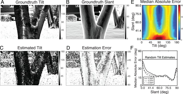
Figure 6 summarizes the overall accuracy of the conditional-means estimates of tilt. Figure 6A shows the ground-truth tilt at each pixel location for an example image. Figure 6B shows the ground-truth slant at each pixel. Figure 6C shows the tilt estimates. Figure 6D shows the (circular) difference between the ground truth tilts and the estimates. Tilt is undefined when slant equals zero, and hence we examined how tilt estimation error changes as a function ground-truth slant and tilt (Figure 6E). The black curve in Figure 6F shows tilt error as a function of ground-truth slant. Tilt error decreases steadily as a function of slant. At slants greater than 45°, the median absolute tilt error is less than 20° (except for the very largest slants). Errors are lowest when the range tilt is near 0° and 90° (Figure 6E), the peaks of the prior distribution (see later).

Figure 6.

Tilt estimation errors. (A) Ground-truth tilt for an example image (cf. Figure 5). (B) Ground-truth slant. Note that the gradient operators used to obtain estimates of ground-truth 3D orientations tend to overestimate slant of pixels near depth boundaries. This effect can be seen in the image regions abutting the foreground tree. (C) Optimal (MMSE) tilt estimates when all three cues are present. (D) Errors in tilt estimates. Tilt errors increase in magnitude as the slant approaches zero. (E) Median absolute tilt estimation errors as a function of ground-truth tilt and slant. For slants near zero, where tilt is undefined, tilt errors are large. Beyond approximately 20°, the pattern of tilt errors becomes nearly invariant to slant. (F) Tilt error as a function of ground-truth slant. As slant increases, tilt estimation error decreases systematically. The solid curve is for an analysis area with a diameter of 0.25°, the analysis area used throughout the rest of the article. At slants greater than 40°, the median tilt estimation error drops to approximately 15°.

The tilt error is large at tilt 45° and 135° because of two factors. First, the cues do not provide particularly good information at those tilts; that is, even though the conditional measurement distributions are centered at those range tilts (Supplementary Figure S2), the distributions are very broad (Supplementary Figure S3). Second, the prior has a large influence on the broad likelihood functions that result from the poor measurements. The combination of these two factors significantly reduces performance at tilts well off the cardinal axes. However, it is important to note that even off the cardinal axes, there are cue conditions in which the estimates of tilt are substantially more accurate (see below).

The figures in this article are primarily based on estimates obtained for a local analysis area having a diameter of 0.25° (Gaussian window with a standard deviation of 0.1°). However, we ran the same analysis for areas with diameters 1.5 and 2.0 times as large (Figure 6F). The results are very similar—nearly all the plots look the same. The primary difference is that larger analysis areas produce somewhat less variable results. This fact indicates that the observed pattern of results is not an accident of the size of the analysis area.

Conditional means: Properties of estimates

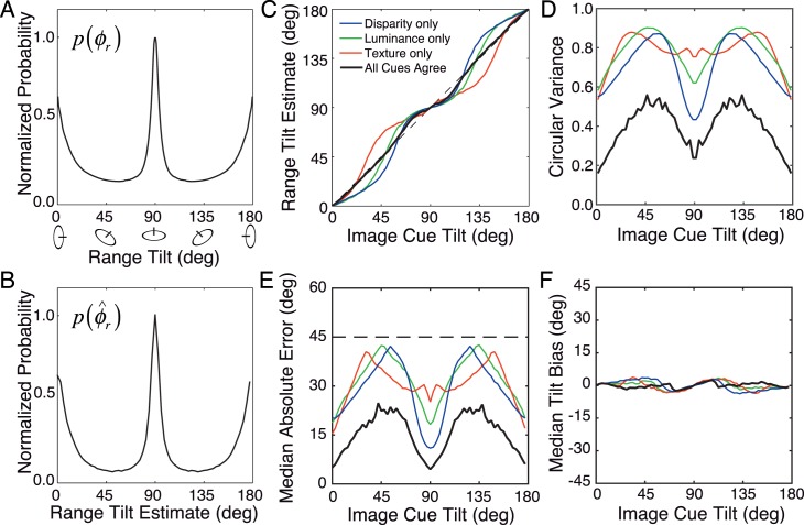
In this subsection, we look in more detail at the properties of the conditional-means estimates. First, we show the prior distribution of 3D tilts in natural scenes (Figure 7A; see later in Results for more detail) and the distribution of optimal three-cue tilt estimates in natural scenes (Figure 7B). Both have prominent peaks at the cardinal tilts but have substantial probability mass at all tilts. Next, we examine the tilt estimates given each image cue value alone. Figure 7C shows the estimate of 3D tilt given the measured value of luminance alone, texture alone, and disparity alone; that is, E(ϕ_r|ϕ_l), E(ϕ_r|ϕ_t), and E(ϕ_r|ϕ_d). For image cue tilt measurements near 0⁰ and 90°, the estimates are equal to the measured cue value. However, for image cue measurements near 45° and 135°, estimates are shifted toward 0° and 90°. This shift is largely due to the effect of the prior. The prior distribution exhibits a strong cardinal bias. Surfaces slanted around horizontal axes (tilt = 90°) or vertical axes (tilt = 0°) are much more likely than other tilts. When only one image cue is measured, the information it provides is not highly reliable (Figure 7D). However, if all three cues are measured and agree, the influence of the prior on the conditional means E(ϕ_r|ϕ_l = ϕ_t = ϕ_d) is nearly eliminated (Figure 7C, black curve), and the estimate reliability increases substantially (Figure 7D, black curve).

Figure 7.

Tilt prior in natural scenes and optimal single-cue tilt estimates, variance, error, and bias. Three-cue performance is also shown for when all three cues agree. (A) Unsigned tilt prior in natural scenes. The tilt prior exhibits a strong cardinal bias. Slants about horizontal axes (tilt = 90°) are most probable (e.g., the ground plane straight ahead). Slants about vertical axes (tilt = 0° and 180°) are the next most probable. All other tilts are much less probable. (B) Distribution of optimal tilt estimates. Its shape is similar to the shape of the tilt prior. (C) Tilt estimates conditioned on individual image cue values and estimates conditioned on cases when all three cues agree. Specifically, blue indicates tilt given disparity alone E(ϕ_r|ϕ_d), green indicates tilt given luminance alone E(ϕ_r|ϕ_l), red indicates tilt given texture alone E(ϕ_r|ϕ_t), and black indicates the expected tilt value when all three cues agree. (D) The precision of the optimal estimates. Disparity alone yields the most reliable estimates for most, but not all, image cue values. When all three image cues agree, the precision of the optimal estimate is significantly increased (see Methods). (E, F) Median absolute error (magnitude) and bias of estimates as a function of image cue value. When all three image cues agree, there is a substantial increase in precision and a decrease in bias.

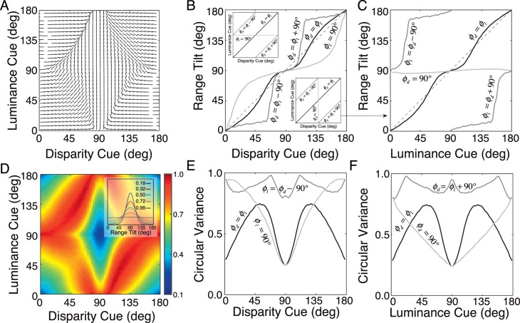
Figure 7E and 7F show how the accuracy and the bias of the tilt estimates vary as function of the image cue value for each of the individual cues (colored curves) and for the case in which the three cue values agree (black curve). When the cue values agree, estimation accuracy is considerably better (in agreement with the reduced bias and variance of the estimates shown in Figure 7C, D). This fact could be exploited by the visual system because the cue values are available to the observer (see Discussion) Next, we examine tilt estimates given both the disparity and luminance cue values. The estimates for all combinations of luminance and disparity cue values, E(ϕ_r|ϕ_l,ϕ_d), are shown in Figure 8A. The pattern of results is intuitive but complex. Depending on the particular values of the disparity and luminance cues, we see several different types of behavior: disparity dominance, cue averaging, and cue switching. For example, when disparity equals 90°, E(ϕ_r|ϕ_l,ϕ_d = 90), we observe disparity dominance; that is, the luminance cue exerts almost zero influence on the estimate (vertical midline of Figure 8A; see Figure 8B inset). On the other hand, when luminance equals 90°, E(ϕ_r|ϕ_l = 90,ϕ_d), the disparity cue exerts a strong influence on the estimate (horizontal midline of Figure 8A). When luminance and disparity agree, E(ϕ_r|ϕ_l = ϕ_d), the single-cue estimates are approximately averaged (positive oblique of Figure 8A). When luminance and disparity disagree by 90°, E(ϕ_r||ϕ_l − ϕ_d| = 90), the best estimates switch from 0° to 90° abruptly when the disparity cue approaches ∼65° and then switches abruptly back from 90° to 0° when the disparity cue approaches ∼115°. All of these effects can be seen more readily by examining the value of the estimate as a function of the disparity cue for different luminance cue values (Figure 8B) and as a function of the luminance cue for different disparity cue values (Figure 8C).

Figure 8.

Two cue optimal estimates and precision. (A) Optimal tilt estimates given disparity and luminance cue values: E(ϕ_r|ϕ_d,ϕ_l). Each line segment indicates the optimal tilt estimate (i.e., the expected tilt value). (B) Expected tilt (replotted from A) as a function of the disparity cue for different luminance cue values (see upper left inset). Specifically, when luminance and disparity cues always agree with each other E(ϕ_r|ϕ_d = ϕ_l), when luminance always equals 90° E(ϕ_r|ϕ_d,ϕ_l = 90), and when luminance and disparity cues differ by 90° E(ϕ_r||ϕ_d, − ϕ_l| = 90). (C) Expected tilt (also replotted from A) but as a function of the luminance cue (see lower right inset in B) for different disparity cue values. When the disparity cue equals 90°, luminance has almost no influence on the optimal estimate (disparity dominance). (D) Estimate precision (circular variance) based on measured disparity and luminance cue values. (Inset: Von mises distributions spanning the range of depicted circular variances.) (E, F) Circular variances for the same conditions as in B, C.

A complex pattern of estimate reliability emerges as well (Figure 8D). Estimates are most reliable when luminance and disparity agree with each other and have values near 0° or 90°. Interestingly, in some regions of the space, estimates are more reliable if the cues disagree than if they agree. For instance, if disparity = 67.5° and luminance = 90°, the tilt estimate is more reliable than if both disparity and luminance agree and have values of 67.5°. Estimates are most unreliable when they differ by 90°.

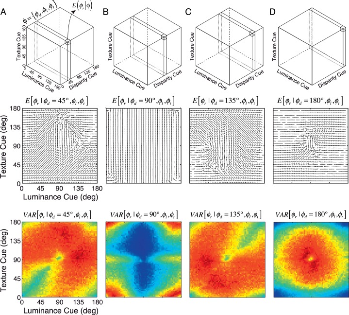
Finally, we examine optimal tilt estimates given all three image-cue values. The three-cue results are even more complicated, but they are richer and more interesting to work through (Figure 9). Consider the optimal estimates given all possible combinations of the luminance and texture cues and one particular value of the disparity cue. The particular combination of luminance and texture values strongly influences the 3D tilt estimates. If the luminance and texture cues significantly differ from each other, the disparity cue dominates (i.e., the optimal estimate very nearly equals the tilt specified by disparity). However, if luminance and texture cues agree, they override the disparity cue. Consider the case in which disparity equals 45° and luminance and texture take on arbitrary values (Figure 9A). When both luminance and texture equal ∼135°, the estimate is very near to 135°, even though the disparity estimate specifies 45°. Now consider the case in which disparity equals 90° (Figure 9B). In this case, estimates from disparity are modified very little by the luminance and texture cues, no matter what their values are. For nearly all combinations of luminance and texture, the best estimate of 3D tilt is approximately 90°. The one exception is when luminance and texture equal each other and also equal 0° (thereby differing from disparity by 90°). When disparity is 135° (Figure 9C) or 180° (Figure 9D), the story is broadly similar to the cases in which disparity equals 45° (Figure 9A) or 90° (Figure 9B), respectively. (See Supplementary Figure S1 for all possible combinations of disparity and luminance cues for each of several particular texture cue values.)

Figure 9.

Three cue optimal estimates and precision, for all values of luminance and texture when A disparity equals 45°, B disparity equals 90°, C disparity equals 135°, and D disparity equals 180°. Top row: The cue cube indicates the plane from which the optimal estimates are shown. Middle row: Line segment orientation indicates the tilt estimate given each particular combination of cue values. Bottom row: Circular variance of optimal estimates. The color bar is the same as in Figure 8D (i.e., circular variance on [0.1 1.0]).

Figure 9 also expands on the finding in Figure 7 that when all three cues agree, estimate precision increases. For example, in the panels in which the disparity cue is 45° and 135°, the precision is seen to be substantially higher whenever both the luminance and texture cues are within a neighborhood of 45° and 135°, respectively.

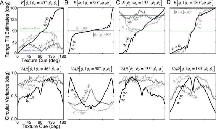
Figure 10 shows slices through the three-cue estimate and precision plots. Interestingly, when disparity equals 90°, the most reliable (lowest variance) estimates occur when the image cues are in conflict (Figure 10B); specifically, when disparity equals 90°, luminance equals 90°, and texture equals 45°, the circular variance of the estimate is approximately 20% lower (0.19 vs. 0.24) than when disparity, luminance, and texture all equal 90° and agree with each other. The same holds true for all texture values between 30° and 80° (when disparity and luminance equal 90°). Can this effect be accounted for by the precision of the single cue estimates? It appears not. The estimate of the precision of the texture alone at 45° is lower than that at 90°. And yet, the precision of the three-cue estimate when texture equals 45° (and luminance and disparity equal 90°) is higher than when texture equals 90°. This behavior is not predicted by standard (linear) models of cue combination and would make an interesting case to test in future psychophysical experiments.

Figure 10.

Three cue estimates (replotted from Figure 9) for specific combinations of luminance and texture when (A) disparity equals 45°, (B) disparity equals 90°, (C) disparity equals 135°, (D) disparity equals 180° (similar to Figure 9). Top row: Surface tilt estimates, for each disparity cue value, when luminance equals texture (black), luminance disagrees with texture by 90° (middle gray), and luminance equals 90° (light gray). For reference, light blue indicates the optimal estimate for conditioned on disparity alone (see above), while light green indicates the optimal estimate conditioned on luminance alone when luminance equals 90°, E(ϕ_r|ϕ_l = 90°). Bottom row: Circular variance for the same conditions.

The detailed manner in which luminance and texture modify the optimal estimate from disparity alone is plotted directly in Figure 11. We show the two most extreme cases: (a) when luminance and texture agree with each other but not necessarily with disparity and (b) when luminance and texture differ by 90°. To highlight the modifying influence of luminance and texture, we plot the difference between the estimate from disparity alone and the estimate from all three cues, for the two cases just mentioned.

Figure 11.

The influence of luminance and texture on tilt estimates from disparity. The difference between the all-cues estimates and disparity-alone estimates is plotted as a heat map. (A) Dramatic departures from the disparity alone estimate occur when luminance and texture agree and differ from disparity (except when disparity equals 90°). (B–E) As the difference between luminance and texture increases from (B) 22.5°, (C) 45.0°, (D) 67.5°, and (E) 90.0°, the influence of luminance and texture progressively decreases. When luminance and texture are in maximal disagreement, |ϕ_l − ϕ_t| = 90°, they have little or no effect; that is, the three-cue estimates are almost the identical to the disparity-alone estimate.

Figure 11A shows that when luminance and texture agree with each other, they strongly affect the optimal estimate from disparity alone, E(ϕ_r|ϕ_d,ϕ_l = ϕ_t) − E(ϕ_r|ϕ_d). When luminance and texture agree, they override disparity unless disparity equals 90° (or unless luminance and texture approximately agree with disparity). Figure 11B, D shows that luminance and texture have progressively less effect as the difference between them increases. Figure 11E shows that when luminance and texture differ by 90°, they have virtually no effect on the optimal estimate (disparity dominance). That is, the difference E(ϕ_r|ϕ_d,|ϕ_l − ϕ_t| = 90°) − E(ϕ_r|ϕ_d) is near zero for virtually all values of disparity, luminance, and texture. Thus, in general, luminance and texture override disparity when they agree and have little effect when they disagree.

Luminance and texture may override disparity because estimates of tilt from disparity can be misleading or inaccurate. For example, disparity estimates near depth boundaries are unreliable because disparity signals are undefined for half-occluded regions of the scene. On the other hand, luminance and texture cues frequently agree with each other at or near depth boundaries and are immune to the half-occlusion problem. Thus, many of the cases in which disparity is overridden by luminance and texture occur near depth boundaries. Note that at depth boundaries, gradient-based slant and tilt estimates will not correspond to individual surfaces. The measure of tilt will therefore provide information about the orientation of a depth boundary and/or the tilt of surfaces. Differentiating between highly slanted surfaces and depth discontinuities in natural scenes is an important research question in its own right.

Linear estimate combination

The Bayes optimal estimates given by the conditional means are the best (in mean squared error) performance possible (for our natural scenes), given the three specific cues defined above. Of course, there are other local and global cues available to the visual system. As noted earlier, it is beyond the scope of this article to consider global cues. However, within a linear summation framework, it is possible to consider additional local cues. The starting point is to compare the conditional-means method with linear estimate combination (Equation 12) for the same three main cues considered above.

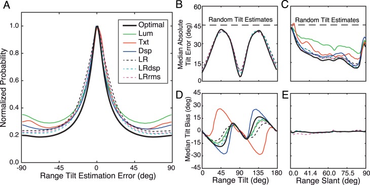
The solid and dashed black curves in Figure 12 plot the overall performance of the two methods. Figure 12A plots the overall distribution of tilt errors. Figure 12B plots the median absolute tilt error of the two methods as a function of tilt and Figure 12C the median absolute tilt error as a function of slant. Although Figure 12B may give the impression that the optimal estimator assigns each patch to only one of the cardinal tilts, this is not the case. The probability distribution of tilt estimates has mass at all tilt values (see Figure 7B) and significantly outperforms a model that assigns only cardinal tilts. Figures 12D and 12E show similar plots for the median signed error. Although the linear estimate combination performs worse overall, its performance is very close to the optimal across all tilts and slants. This result shows that the simpler linear estimate combination can capture most of the information captured by the optimal method and provides some justification for using the linear estimation combination to evaluate human performance with natural stimuli. This result also provides some justification for using the linear-cue combination framework to evaluate the effect of additional cues.

Figure 12.

Comparison of the optimal conditional-means method and other estimators. (A) Grand histogram of errors for the optimal (black), luminance gradient cue only (green), texture gradient cue only (red), disparity gradient cue only (blue), linear reliability–based cue combination (dashed black), linear reliability–based cue combination with local disparity-specified distance as the auxiliary cue (dashed cyan), and linear reliability–based cue combination with local RMS contrast as the auxiliary cue (dashed cyan). (B) Mean absolute error as a function of ground-truth tilt. (C) Mean absolute error as a function of range slant (cf. Figure 6F). (D) Median tilt bias as a function of range tilt. (E) Median tilt bias as a function of range slant. To reduce clutter, the single-cue results are not shown in B and E.

The simplicity of the linear estimate combination allows one to examine the potential impact of additional local cues. We chose to examine three simple local auxiliary cues available to the early visual system: the mean disparity (i.e., vergence demand) δ̄, the mean luminance l̄, and the RMS contrast c̄. Each of these is a weighted average computed over the same analysis area as the three main cues and can take on an arbitrary value v. 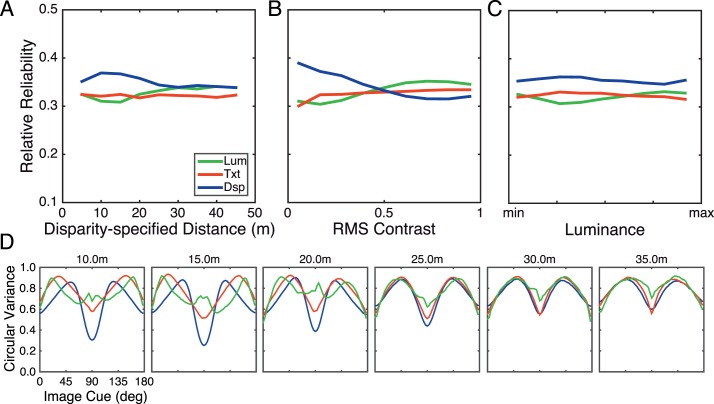To evaluate the information provided by each of these auxiliary cues, we computed the single-cue estimates and their variances (and hence reliabilities), conditional on the value of the tilt cue and the value v of the auxiliary cue: Φ̂_r|δ,v = E(ϕ_r|ϕ_δ,v), = VAR(ϕ_r|ϕ_δ,v), Φ̂_r|l,v = E(ϕ_r|ϕ_l,v), = VAR(ϕ_r|ϕ_l,v), Φ̂_r|t,v = E(ϕ_r|ϕ_t,v), = VAR(ϕ_r|ϕ_t,v). To illustrate the broad effects of these cues, Figures 13A-C plot the average relative reliability for the three main cues as a function of each of the auxiliary variables. As can be seen, the average relative reliability of tilt estimates from disparity decreases with absolute disparity and rms contrast, but the average relative reliability of the other estimators is largely unaffected by these auxiliary cues. Note that for very large distances, disparity can play no role because then changes in depth will create changes in disparity below the disparity detection threshold. Luminance has very little effect on any of the estimators. This result is intuitive. In general, the disparity gradient information should decrease with distance because of the inverse square relationship between disparity and distance. We suspect that the disparity reliability decreases with RMS contrast in natural scenes because high-contrast regions are correlated with depth discontinuities and because disparity information is generally poor at depth discontinuities (i.e., high-disparity gradients). Figure 13D shows how the variability of the individual cue values (across tilt) changes with the disparity-defined distance in meters.

Figure 13.

Relative reliability of each individual gradient cue, averaged across tilt, as a function of different local auxiliary cues. (A) Disparity-specified distance. (B) RMS contrast. (C) Luminance. The averages across tilt are simply for purposes of illustrating broad trends. (D) Variance of each individual gradient cue estimator across tilt for different disparity-specified distances. The average relative reliability in A is obtained by computing the average inverse variance across tilt at a given disparity-specified distance.

The dashed colored curves in Figure 12 show the performance of the linear estimate combination when the auxiliary cues of absolute disparity (dashed light blue) and RMS contrast (dashed red) are included. There is a small improvement in tilt estimation accuracy when these local auxiliary cues are used.

The properties of the estimates produced by the linear estimate combination are very similar in most respects to the properties of the conditional-means estimates shown in Figures 8 to 11. However, there are some subtle differences that could be compared with human tilt judgments on the same stimuli. The clearest example concerns the distinction between cue vetoing and cue averaging. One of the interesting properties of the conditional-means estimates is that in some cases, they correspond to something like the average of the estimates from the three cues alone, but in other cases, one or more of the single-cue estimates is effectively vetoed by the other estimate or estimates. This behavior is sensible. For example, if the estimates from the three cues are similar, then it is sensible to average them. However, if one cue gives an estimate that is far from the other two, then averaging it in will pull the estimate to a value that is not close to the estimate of from any of the cues. In this case, it makes intuitive sense to ignore the outlier (Knill, 2007). This vetoing effect is illustrated in Figure 14. The black curve shows the optimal estimate when the luminance and texture cues agree and the disparity cue is fixed at 45°. If the disparity cue were being completely ignored, the estimates would fall on the diagonal (dashed line). Thus, the plot shows that the disparity cue is essentially vetoed for most of the luminance/texture cue values. This occurs even though the reliability of the disparity cue at a tilt of 45° is usually greater than the reliability of either of the other two cues (see Figure 7C). Linear estimate combination, on the other hand, does only weighted averaging. If one cue has sufficiently low reliability compared with the other cues, it is effectively vetoed; however, as the dashed curve in Figure 14 shows, it does not have the same vetoing power as the conditional-means estimator. For luminance/texture tilts in the range of 70° to 130°, the disparity cue pulls the estimate toward 45°. It should be possible in psychophysical experiments, using these same natural stimulus patches, to determine whether the human tilt estimates are more like those of linear estimate combination or conditional means.

Figure 14.

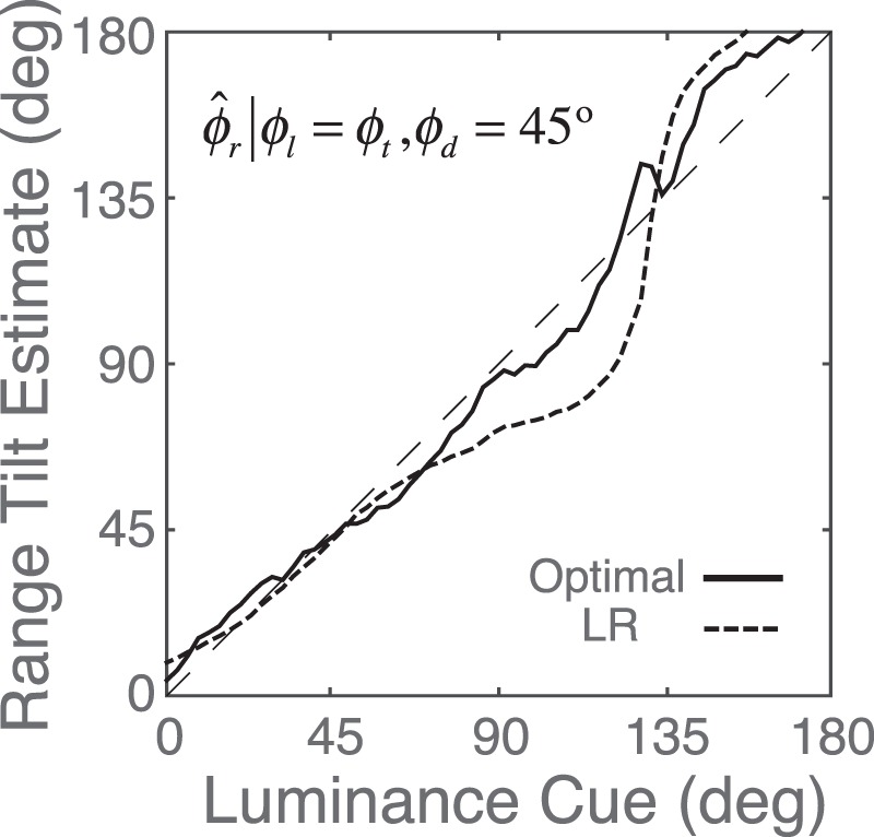
Tilt estimates when the luminance and texture cues are equal and the disparity cue signals a tilt of 45°. If the disparity cue is vetoed (ignored), the estimates should fall on the dashed line. The black curve shows the MMSE optimal estimates, which largely veto disparity when luminance and texture agree. The dashed black curve shows the estimates based on linear cue combination (the LR estimator). For the LR estimator, disparity pulls the estimates in the direction of 45° when luminance/texture cue is in the range of 70° to 130°.

Prior distribution of slant and tilt in natural scenes

The distribution of local 3D orientations in natural scenes can be represented by a joint prior over slant and tilt. Slant and tilt are spherical coordinates (i.e., a surface normal is a vector on the unit sphere); a uniform distribution of slant and tilt, therefore, corresponds to a flat distribution on the surface of the unit hemisphere. Most high-level programming languages do not have off-the-shelf methods for computing histograms on equal area bins on the surface of a sphere. Thus, to accurately measure the distribution of slant and tilt with widely available tools, it is necessary to perform an area-preserving cylindrical projection of the measured joint slant-tilt values (Rosenberg, Cowan, & Angelaki, 2013). In the projection, tilt is represented directly ϕ_r → and slant is represented by the cosine of the slant cos θ_r → , where * indicates the representation of the coordinate in the projection. The projection is area preserving in that the uniformity of surface orientations on the sphere (cf. Figure 1) implies uniformity in the projection and vice versa.

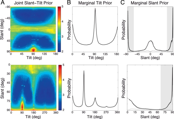
The joint prior distribution is shown in Figure 15A. The marginal prior distributions over tilt and over slant are shown in Figure 15B, C. Consistent with previous findings, we find a strong cardinal bias in the marginal tilt distribution. Specifically, tilts that are consistent with the ground plane straight ahead (90°) are most probable; tilts that are consistent with surfaces slanted about vertical axes (0° and 180°), such as tree trunks, signposts, and buildings, are next most probable.

Figure 15.

Slant-tilt prior in natural scenes, for two equivalent parameterizations of slant and tilt. Upper row: tilt = [0 180), slant = [−90 90); lower row: tilt = [0 360), slant = [0 90). A joint prior distribution of slant-tilt in natural scenes. The color bar indicates the count in log₁₀ (e.g., 5 indicates a count of 10⁵); some slant-tilt combinations are ∼100× more likely than others. High slants at tilt = 90° (e.g., ground plane straight ahead) are most probable. Slant zero surfaces are also quite probable (where tilt is undefined). (B) The marginal tilt prior distribution. (The upper plot is exactly the same data as Figure 7B). (C) The marginal slant prior distribution. The dashed black curve is a mixture of Gaussians fit to the slant prior (see Appendix for parameters). The gray curve is the marginal slant distribution computed without an area-preserving projection. The shaded areas (|slant| > 67.5°) indicate results that may be due to depth discontinuities rather than the surfaces of individual objects.

As has been previously reported, the prior slant distribution is highly nonuniform (Yang & Purves, 2003). However, previous studies have reported that surfaces near 0° of slant are exceedingly rare in natural scenes (Yang & Purves, 2003), whereas we find significant probability mass near 0° of slant. That is, we find—consistent with intuition—that it is not uncommon to observe surfaces that have zero or near-zero slant in natural scenes (e.g., frontoparallel surfaces straight ahead). Further, we find that for slants less than 67.5°, the prior is well approximated by a mixture of two Gaussian distributions (see the Appendix for best-fit parameters).

What accounts for the differences between our results and those previously reported? The primary difference appears to be due to how the 3D orientation is projected. If one does not perform a projection that preserves area on the unit sphere (i.e., if one bins on θ_r rather than on cos (θ_r)), the estimated marginal slant distribution is dramatically different. The slant prior distribution computed without an area-preserving projection has effectively zero probability mass near zero. Taken at face value, such a result would lead to the erroneous conclusion that surfaces with slants near zero almost never occur in natural scenes (Figure 15C, gray curves).

Note that the gradient operator method used to obtain estimates of ground-truth 3D orientations tends to overestimate surface slant near depth boundaries (cf. Figure 6B). We strongly suspect that this effect accounts for the rapid increase in probability mass near 90°. This is why the plots in Figure 15C have been shaded. However, this inaccuracy is unlikely to substantially affect the primary conclusions of this article because the tilts near depth edges are typically orthogonal to the depth boundary. Nevertheless, a more sophisticated method for estimating local surface orientation from databases with ground-truth distance data is clearly an important subject for future research.

Discussion

Estimating the local 3D orientation is a precursor to estimating 3D shape. Local 3D orientation is parameterized by slant and tilt. Our primary aim was to determine the optimal estimates of local tilt given the measured values of several simple image cues, where the goal is to minimize the squared error with the ground-truth 3D tilt.

We accomplished this aim by first collecting a large database of calibrated stereo-images of natural scenes with co-registered range data. Next, we measured three image cues (orientation of disparity gradient, orientation of luminance gradient, and dominant texture orientation) as well as the ground-truth slant and tilt in the range images for every pixel in the database (ground truth is defined as the local gradient of the range image). Then, we computed the optimal (MMSE) estimate of tilt for all possible combinations of the disparity, luminance, and texture cues using the conditional means method. A rich set of results emerged. The results show that very local (0.25°), very simple image cues can be used to obtain moderately accurate estimates of tilt. More specifically, we find that (a) the optimal estimates for each single cue are somewhat biased, because of the peaks in the prior distribution at horizontal and vertical tilts; (b) the precision of tilt estimates generally increases with slant; (c) binocular disparity is the most reliable of the tested cues; but (d) if the estimates from luminance and texture cues agree and are different from the estimate from the disparity cue, then the luminance and texture cues override the disparity cue; and, more generally, (e) when the values of the three cues are approximately the same, the tilt estimates are more accurate, and the precise (f) optimal cue combination in natural scenes often appears to involve complex nonlinear interactions.

We then compared estimates from the conditional means (Bayes optimal) method with those of the linear estimate combination. We found that the overall performance of the linear estimate combination is only slightly below that of the conditional means, although it displays weaker cue-vetoing behavior under some circumstances. An advantage of the linear estimation combination is that it allows analysis of a larger number cues for the same amount of data. This allowed us to measure the usefulness of several other auxiliary cues (measured at the same location as the three main cues): mean absolute disparity, mean luminance, and RMS contrast. In agreement with intuition, we found that the absolute disparity was the most useful auxiliary cue—as the absolute disparity decreases (i.e., distance increases) the weight given to the disparity gradient orientation cue is reduced.

Cost function

In determining the optimal estimates, we assumed that the goal is to minimize the squared error between the estimated tilt and the ground-truth tilt. We chose this goal (cost function) for two reasons. First, with this goal, the cost grows smoothly with the magnitude of the error, in agreement with the intuition that survival costs in the real world are less on average if the behavior is close to what was intended. Second, this optimal estimation rule can be learned by directly measuring the conditional mean for each combination of cue values, without making any assumptions about the underlying joint four-dimensional distribution. Requiring only the conditional means made it practical to learn the optimal estimation rule directly from our set of registered range and camera images.

Another simple cost function is one that treats all errors as equally bad. This cost function, which produces maximum a posteriori (MAP) estimates, is less appropriate for many estimation tasks because it does not give credit for being close to the correct estimate. Another limitation of this cost function is that it requires characterizing the posterior distributions sufficiently to determine the mode, which, because of data limitations, would be impossible without strong assumptions about the form of the joint distribution. However, MAP estimates are appropriate for other tasks such as recognition of specific objects or faces, in which close does not count. Also, if the likelihood distributions are symmetrical about the peak (e.g., Gaussian), the MAP and MMSE estimates are the same. Finally, for certain strong assumptions (e.g., statistical independence of the cue distributions), it is widely believed that MAP estimators are more biologically plausible.

Linear estimate combination

Although minimizing the squared error is a sensible cost function, it seems unlikely that the visual system learns a separate specific conditional mean for every possible triplet of cue values. Thus, it is important to consider whether there are simpler computations that could closely approximate the Bayes optimal estimate. Psychophysical (Burge et al., 2010b; Hillis et al., 2004; Knill & Saunders, 2003) and neurophysiological studies (Murphy, Ban, & Welchman, 2013; Rosenberg & Angelaki, 2014; Sanada, Nguyenkim, & DeAngelis, 2012; Tsutsui, Jiang, Yara, Sakata, & Taira, 2001; Welchman, Deubelius, Conrad, Bülthoff, & Kourtzi, 2005) have investigated how cues are combined in estimating surface orientation. Some of these studies have demonstrated that behavioral and neural responses are consistent with linear summation with weights given by relative reliability (Burge et al., 2010b; Hillis et al., 2004; Knill & Saunders, 2003; Sanada et al., 2012). However, these studies used artificial laboratory stimuli. The present analysis of cue combination in natural images shows that linear summation using relative reliability is near optimal in our natural images (Figure 12), at least for the specific cues and local analysis areas (0.25°–0.50° diameter areas) examined here. This finding would seem to help explain why biological systems have evolved cue combination mechanisms consistent with this simple rule.

Limitations and directions

The present study focused exclusively on how to combine cues measured at the same location in static stereo natural images. Although much of the power of the human visual system must derive from more global cues and integration mechanisms, the visual system starts with local measurements. The better the initial local estimates of tilt, the more effective will be global cues and integration mechanisms that build on them. Thus, there has undoubtedly been evolutionary pressure to optimize local cue combination at single locations in natural scenes, and hence it is sensible to consider how to combine cues at single locations in natural scenes. Also, it is possible to compare human and optimal performance under conditions in which only local cues are available.

The main cues and auxiliary cues considered here were picked because they are simple and likely to reflect computations in the early levels of the visual system. We might expect evolution (or learning over the life span) to select local cues that provide the best information for tilt estimation in natural scenes. This raises the question of whether there are substantially better local cues than the ones we chose.

The texture cue that we used (the major axis of the amplitude spectrum) is nonstandard (but see Fleming, Holtmann-Rice, & Bulthoff, 2011); it is formally appropriate only for locally isotropic textures (statistically the same in all directions). It is therefore fair to question whether tilt estimation from texture alone could be improved with a more traditional texture cue. We evaluated a more standard cue based on the local gradient in spatial frequency (Clerc & Mallat, 2002; Galasso & Lasenby, 2007; Malik & Rosenholtz, 1997). This cue is appropriate for locally anisotropic (but statistically stationary) textures. The particular version we used is similar to Massot and Hérault (2008). At each pixel location, the amplitude spectrum is computed in the same way as for the major-axis cue (see Methods). The amplitude spectrum is then filtered to reduce low spatial frequencies (e.g., luminance gradients) and enhance mid and high frequencies. Next, the centroid spatial frequency f̄ is computed. The result of this computation at each pixel location is a centroid-frequency image. Finally, we compute the gradient of the centroid-frequency image and define the tilt cue as the orientation of the centroid gradient:

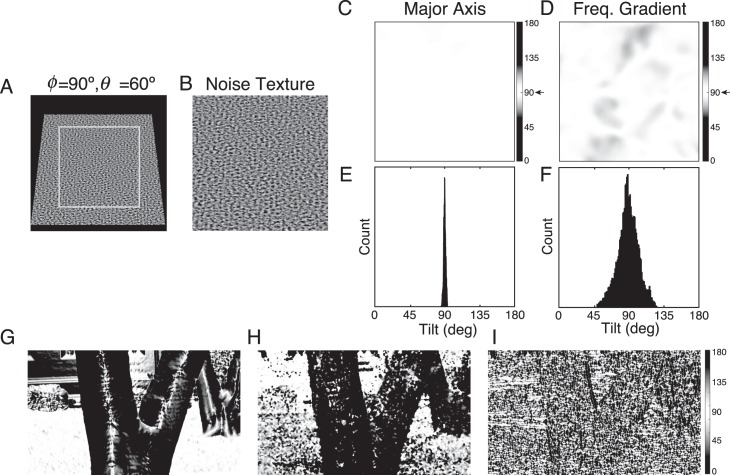
Figure 16A–F shows a comparison of the tilt estimates for the major-axis cue and the centroid cue for a synthesized surface textured with noise. The noise texture (Figure 16A, B) consisted of 200 random frequency and phase components having amplitudes that fall inversely with frequency (similar to the amplitude spectra of natural images). For this (and other) isotropic noise textures, the major axis cue is much more reliable than the centroid cue (compare Figures 16C, E and 16D, F). We also considered a more sophisticated texture gradient cue similar to that of Malik and Rosenholtz (1997). It performed slightly better than the centroid cue but still much worse than the major-axis cue. This is not surprising given that the centroid cue involves computing the derivatives of noisy data.

Figure 16.

Comparison of texture cues for tilt estimation. (A, B) Synthesized image of a planar textured surface with a slant of 60° and a tilt of 90°. (C) Map of the tilt estimated at each pixel location in B for the major axis cue used here. The map is all white because the major axis of the spectrum is 90° at all locations. (D) Map of the tilt estimated at each pixel location in B for the frequency centroid gradient cue. (E, F) Histograms of the tilt estimates for the two cues. (G) Map of ground-truth tilt at each pixel location of an example natural image. (H) Map of estimated tilts for example natural image using major axis cue. (I) Map of estimated tilts for example image using frequency centroid gradient cue.

Interestingly, the major-axis cue is also more reliable for our natural images (see example in Figure 16G–I), even though natural-image textures are generally not isotropic. The most likely explanation is that outdoor images such as those in our data set are sufficiently isotropic for the major-axis cue to outperform the noisier centroid cue. We speculate that for images like those in our data set, there is unlikely to be a local texture cue much better than the major axis cue.

For purely local measures, there are no obvious alternatives to the disparity and luminance gradient cues. It may be possible to use other techniques to find the most useful local image features for tilt estimation (Burge & Geisler, 2011, 2012, 2014, 2015; Geisler, Najemnik, & Ing, 2009); however, it seems likely (given our past experience) that any improvements in performance would be modest.

One slightly puzzling fact is that the luminance cue is as good as (or better than) the texture cue (note the bias and reliability in Figure 7), even though luminance gradients are not typically considered to be cues for tilt. One contributing factor may be that at surface boundaries, the tilt of the foreground object tends to be orthogonal to the boundary. This would be true for cylinders and would seem likely to be more generally true (e.g., wherever surface boundaries are locally conic, as they are for foliage branches). This would create a correlation between the luminance edge created by the boundary and the tilt of the foreground surface at and near the boundary. However, the usefulness of luminance cannot entirely be due to surface boundaries because the luminance cue still provides information about tilt for ground-truth slants much smaller than 90° (e.g., Figure 12C).

The relatively poor overall performance of the optimal and linear estimate combination for the tilt and auxiliary cues considered here (e.g., Figure 12) is consistent with the subjective impression of viewing natural scenes through a small aperture (and with psychophysical measurements; Kim & Burge, 2016). Nonetheless, the set of properties and the performance of the optimal and linear cue combination computations discovered here provide a rich set of predictions and hypotheses that can be tested in experiments in which only local image patches are presented to observers. An obvious next step is to test these predictions and hypotheses in psychophysical studies.

Although tilt estimates based on either optimal or linear combination of cues at a single location are typically not very accurate, there are large subsets of locations where the estimates are substantially more accurate. We have not fully explored the cases in which the estimates are more accurate, but they include the case in which values of the three main cues are similar (Figures 7 and 9). Image cue values are (of course) available to a visual system. Hence, a visual system could identify those locations where the estimates are likely to be more accurate. Thus, a plausible hypothesis is that these locations are given more weight in the spatial integration mechanisms that incorporate smoothness and other constraints to estimate surface shape. We conclude that the results and database presented here also provide a useful starting point for investigating the global cues and spatial integration mechanisms underlying the perception of 3D surface orientation.

Conclusion

We collected a database of 96 high-resolution calibrated stereo-images together with precise range (distance) measurements at each pixel location and then used this database to evaluate the usefulness of local image cues (disparity, luminance, and texture) for estimating 3D tilt. An assumption-free conditional-means approach was used to determine the optimal (i.e., MMSE) estimates from the three cue values at the same single location. We also evaluated a less optimal, but more plausible, linear cue combination approach. These analyses of natural scene statistics revealed a number of principled and testable hypotheses for the mechanisms underlying 3D orientation perception in natural scenes.

Appendix

Circular statistics: Means, variances, and the Von Mises function

Circular variables can be expressed as complex numbers of unit magnitude (i.e., vectors on the unit circle). The conditional mean for a circular variable is

where ϕ is a vector of cue values, Φ̄_r is the mean angle, and Ā_r is the length of the mean vector. The mean angle is given by the argument of the vector sum

and the length of the mean vector is given by the complex absolute value of the mean vector

The circular variance is a statistic that measures the dispersion (i.e., the spread of the distribution) of a circular variable and is given by

The geometric interpretation of these equations is shown in Figure A1. As the circular variance increases, the length of the mean resultant vector decreases. If the samples of a circular variable are distributed uniformly on the unit circle, the mean resultant vector would be of length zero and the circular variance would equal its maximum value (1.0).

Figure A1.

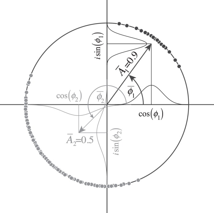
Geometry of circular variables. To compute the average from samples of a circular variable, the (four-quadrant) arc tangent is computed from the average cosine and the average sine of the sample angles. The angle of the average resultant vector is the mean angle and one minus the magnitude of the resultant vector is the circular variance. Plotted are samples from two distributions with different means and circular variances (black and gray symbols).

Figure A2.

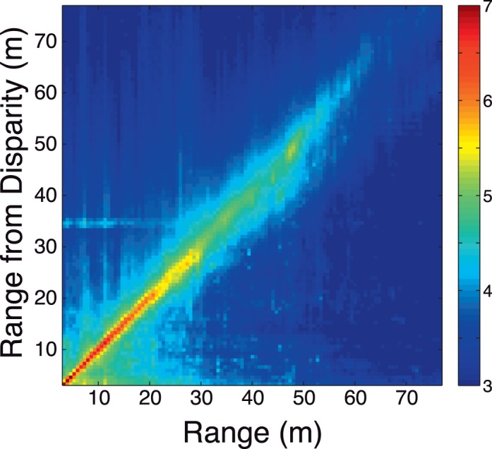
Range estimates from disparity. (A) Histogram of range from disparity estimates against ground-truth range. The color bar indicates the log-base-10 number of samples in each bin. The fact that nearly all the samples are on the positive oblique indicates that the disparity estimation routine (Equation A7) is largely accurate. (B) Mean (solid black curve) and median (black dashed curve) range estimates from disparity as a function of distance. Error bars show 68% confidence intervals of the mean.

The Von Mises distribution (Gaussian on the circle) is given by

where Φ̄ is the mean, κ determines the circular variance, σ² = 1 − I₁(κ)/I₀(κ), and I₀(κ) and I₁(κ) are modified Bessel functions of orders zero and one. Note that given an estimate of σ², we can obtain an estimate of κ by solving the equation I₁(κ̂)/I₀(κ̂) = 1 − σ̂².

Slant prior in natural scenes

The slant prior in natural scenes is presented in Figure 15 in the main text. For slants less than ∼65°, the slant prior is well approximated by a mixture of Gaussian distributions

where σ₁ is the standard deviation of the first Gaussian, σ₂ is the standard deviation of the second Gaussian, and α is a mixing parameter, which is constrained to lie on [0 1]. The best-fit values are σ₁ = 10°, σ₂ = 42°, and α = 0.5. (Note that a mixture of Von Mises distributions also provides a good approximation to the slant prior, where κ₁ and κ₂ are the concentration parameters of the two distributions. The best-fit values are κ₁ = 8, κ₂ = 0.8, and α = 0.5.)

Disparity estimation

Disparity was estimated from the left and right eye luminance images via windowed normalized cross-correlation. Both left and right images were used as reference images, so disparity estimates were obtained for each image:

where L̄ is the local mean of the left image, R̄ was the local mean of the right image, and g(x,y) is a Gaussian window. Negative disparities indicate uncrossed disparities; positive disparities crossed disparities. The estimated disparity was the offset that maximized the correlation between the left and right eye patches.

We verified the accuracy of these disparity estimates against the ground-truth range data by computing the range from the disparity estimates via triangulation based on the geometry of image capture. Figure A2 shows a histogram of range estimates from disparity as a function of the true range. The histogram shows that disparity estimates are accurate out to a distance of at least 50 m.

References

- Alais D,, Burr D. (2004). The ventriloquist effect results from near-optimal bimodal integration. Current Biology, 14, 257–262, http://doi.org/10.1016/j.cub.2004.01.029. [DOI] [PubMed] [Google Scholar]
- Backus B. T,, Banks M. S. (1999). Estimator reliability and distance scaling in stereoscopic slant perception. Perception, 28, 217–242. [DOI] [PubMed] [Google Scholar]
- Banks M. S,, Gepshtein S,, Landy M. S. (2004). Why is spatial stereoresolution so low? Journal of Neuroscience, 24, 2077–2089. Retrieved from http://doi.org/10.1523/JNEUROSCI.3852-02.2004 [DOI] [PMC free article] [PubMed] [Google Scholar]
- Blake A,, Bulthoff H. H,, Sheinberg D. (1993). Shape from texture: Ideal observers and human psychophysics. Vision Research, 33, 1723–1737. [DOI] [PubMed] [Google Scholar]
- Burge J,, Fowlkes C. C,, Banks M. S. (2010a). Natural-scene statistics predict how the figure-ground cue of convexity affects human depth perception. Journal of Neuroscience, 30, 7269–7280. Retrieved from http://doi.org/10.1523/JNEUROSCI.5551-09.2010 [DOI] [PMC free article] [PubMed] [Google Scholar]
- Burge J,, Geisler W. S. (2011). Optimal defocus estimation in individual natural images. Proceedings of the National Academy of Sciences, USA, 108, 16849–16854. Retrieved from http://doi.org/10.1073/pnas.1108491108 [DOI] [PMC free article] [PubMed] [Google Scholar]
- Burge J,, Geisler W. S. (2012). Optimal defocus estimates from individual images for autofocusing a digital camera. Presented at the Proceedings of the IS&T/SPIE 47th Annual Meeting, Proceedings of SPIE: Retrieved from http://doi.org/10.1117/12.912066 [Google Scholar]
- Burge J,, Geisler W. S. (2014). Optimal disparity estimation in natural stereo images. Journal of Vision, 14 (2): 2, 1–18, doi:10.1167/14.2.1. [PubMed] [Article] [DOI] [PMC free article] [PubMed] [Google Scholar]
- Burge J,, Geisler W. S. (2015). Optimal speed estimation in natural image movies predicts human performance. Nature Communications, 6, 7900 Retrieved from http://doi.org/10.1038/ncomms8900 [DOI] [PMC free article] [PubMed] [Google Scholar]
- Burge J,, Girshick A. R,, Banks M. S. (2010b). Visual-haptic adaptation is determined by relative reliability. Journal of Neuroscience, 30, 7714–7721. Retrieved from http://doi.org/10.1523/JNEUROSCI.6427-09.2010 [DOI] [PMC free article] [PubMed] [Google Scholar]
- Clark J. J,, Yuille A. L. (1990). Data fusion for sensory information processing systems. Boston: Kluwer Academic Publishers. [Google Scholar]
- Clerc M,, Mallat S. (2002). The texture gradient equation for recovering shape from texture. IEEE Transactions on Pattern Analysis and Machine Intelligence, 24, 536–549. [Google Scholar]
- Ernst M. O,, Banks M. S. (2002). Humans integrate visual and haptic information in a statistically optimal fashion. Nature, 415, 429–433. Retrieved from http://doi.org/10.1038/415429a [DOI] [PubMed] [Google Scholar]
- Fleming R. W,, Holtmann-Rice D,, Bulthoff H. H. (2011). Estimation of 3D shape from image orientations. Proceedings of the National Academy of Sciences, USA, 108, 20438–20443. Retrieved from http://doi.org/10.1073/pnas.1114619109/-/DCSupplemental [DOI] [PMC free article] [PubMed] [Google Scholar]
- Fleming R. W,, Torralba A,, Adelson E. H. (2004). Specular reflections and the perception of shape. Journal of Vision, 4 (9): 2, 798–820, doi:10.1167/4.9.10. [PubMed] [Article] [DOI] [PubMed] [Google Scholar]
- Galasso F,, Lasenby J. (2007). Shape from texture: Fast estimation of planar surface orientation via Fourier analysis. Proceedings of the British Machine Vision Conference, 71.1–71.10, doi:10.5244/C.21.71.
- Geisler W. S,, Najemnik J,, Ing A. D. (2009). Optimal stimulus encoders for natural tasks. Journal of Vision, 9 (13): 2, 1–16, doi:10.1167/9.13.17. [PubMed] [Article] [DOI] [PMC free article] [PubMed] [Google Scholar]
- Gepshtein S,, Burge J,, Ernst M. O,, Banks M. S. (2005). The combination of vision and touch depends on spatial proximity. Journal of Vision, 5 (11): 2, 1013–1023, doi:10.1167/5.11.7. [PubMed] [Article] [DOI] [PMC free article] [PubMed] [Google Scholar]
- Hillis J. M,, Ernst M. O,, Banks M. S,, Landy M. S. (2002). Combining sensory information: Mandatory fusion within, but not between, senses. Science, 298, 1627–1630. [DOI] [PubMed] [Google Scholar]
- Hillis J. M,, Watt S. J,, Landy M. S,, Banks M. S. (2004). Slant from texture and disparity cues: Optimal cue combination. Journal of Vision, 4 (12): 2, 967–992, doi:10.1167/4.12.1. [PubMed] [Article] [DOI] [PubMed] [Google Scholar]
- Kim S,, Burge J. (2016). Human tilt estimation in local patches of natural stereo-images. Journal of Vision, 16 (12): 1413, doi:10.1167/16.12.1413 [Abstract]. [Google Scholar]
- Knill D. C. (1998a). Ideal observer perturbation analysis reveals human strategies for inferring surface orientation from texture. Vision Research, 38, 2635–2656. [DOI] [PubMed] [Google Scholar]
- Knill D. C. (1998b). Surface orientation from texture: ideal observers, generic observers and the information content of texture cues. Vision Research, 38, 1655–1682. [DOI] [PubMed] [Google Scholar]
- Knill D. C. (2007). Robust cue integration: A Bayesian model and evidence from cue-conflict studies with stereoscopic and figure cues to slant. Journal of Vision, 7 (7): 2, 1–24, doi:10.1167/7.7.5. [PubMed] [Article] [DOI] [PubMed] [Google Scholar]
- Knill D. C,, Saunders J. A. (2003). Do humans optimally integrate stereo and texture information for judgments of surface slant? Vision Research, 43, 2539–2558. Retrieved from http://doi.org/10.1016/S0042-6989(03)00458-9 [DOI] [PubMed] [Google Scholar]
- Landy M. S,, Maloney L. T,, Johnston E. B,, Young M. (1995). Measurement and modeling of depth cue combination: in defense of weak fusion. Vision Research, 35, 389–412. [DOI] [PubMed] [Google Scholar]
- Malik J,, Rosenholtz R. (1994). Recovering surface curvature and orientation from texture distortion: A least squares algorithm and sensitivity analysis. Computer Vision—ECCV' 94, 351–364. [Google Scholar]
- Malik J,, Rosenholtz R. (1997). Computing local surface orientation and shape from texture for curved surfaces. International Journal of Computer Vision, 23 (2), 149–168.
- Mamassian P,, Knill D. C,, Kersten D. (1998). The perception of cast shadows. Trends in Cognitive Sciences, 2, 288–295. [DOI] [PubMed] [Google Scholar]
- Massot C,, Hérault J. (2008). Model of frequency analysis in the visual cortex and the shape from texture problem. International Journal of Computer Vision, 76, 165 Retrieved from http://doi.org/10.1007/s11263-007-0048-x [Google Scholar]
- Mittelstaedt H. (1983). A new solution to the problem of the subjective vertical. Die Naturwissenschaften, 70, 272–281. [DOI] [PubMed] [Google Scholar]
- Mittelstaedt H. (1986). The subjective vertical as a function of visual and extraretinal cues. Acta Psychologica, 63, 63–85. [DOI] [PubMed] [Google Scholar]
- Murphy A. P,, Ban H,, Welchman A. E. (2013). Integration of texture and disparity cues to surface slant in dorsal visual cortex. Journal of Neurophysiology, 110, 190–203. Retrieved from http://doi.org/10.1152/jn.01055.2012 [DOI] [PMC free article] [PubMed] [Google Scholar]
- Murray R. F,, Morgenstern Y. (2010). Cue combination on the circle and the sphere. Journal of Vision, 10 (11): 2, 1–11, doi:10.1167/10.11.15. [PubMed] [Article] [DOI] [PubMed] [Google Scholar]
- Nienborg H,, Bridge H,, Parker A. J,, Cumming B. G. (2004). Receptive field size in V1 neurons limits acuity for perceiving disparity modulation. Journal of Neuroscience, 24, 2065–2076. Retrieved from http://doi.org/10.1523/JNEUROSCI.3887-03.2004 [DOI] [PMC free article] [PubMed] [Google Scholar]
- Ogle K. N. (1952). On the limits of stereoscopic vision. Journal of Experimental Psychology, 44, 253–259. Retrieved from http://doi.org/10.1037/h0057643 [DOI] [PubMed] [Google Scholar]
- Palmer S. E,, Ghose T. (2008). Extremal edges: A powerful cue to depth perception and figure-ground organization. Psychological Science, 19, 77–84. Retrieved from http://doi.org/10.1111/j.1467-9280.2008.02049.x [DOI] [PubMed] [Google Scholar]
- Peterson M. A,, Gibson B. S. (1993). Shape recognition inputs to figure-ground organization in three-dimensional displays. Cognitive Psychology , 25), 383–429. Retrieved from http://www.sciencedirect.com/science/article/pii/S0010028583710108
- Potetz B,, Lee T. S. (2003). Statistical correlations between two-dimensional images and three-dimensional structures in natural scenes. Journal of the Optical Society of America. A, Optics, Image Science, and Vision , 20), 1292–1303. [DOI] [PubMed]
- Rosenberg A,, Angelaki D. E. (2014). Reliability-dependent contributions of visual orientation cues in parietal cortex. Proceedings of the National Academy of Sciences, USA, 111, 18043–18048. Retrieved from http://doi.org/10.1073/pnas.1421131111 [DOI] [PMC free article] [PubMed] [Google Scholar]
- Rosenberg A,, Cowan N. J,, Angelaki D. E. (2013). The visual representation of 3D object orientation in parietal cortex. Journal of Neuroscience, 33, 19352–19361. Retrieved from http://doi.org/10.1523/JNEUROSCI.3174-13.2013 [DOI] [PMC free article] [PubMed] [Google Scholar]
- Sanada T. M,, Nguyenkim J. D,, DeAngelis G. C. (2012). Representation of 3-D surface orientation by velocity and disparity gradient cues in area MT. Journal of Neurophysiology , 107), 2109–2122. Retrieved from http://doi.org/10.1152/jn.00578.2011 [DOI] [PMC free article] [PubMed]
- Saxena A,, Chung S. H,, Ng A. Y. (2008). 3-d depth reconstruction from a single still image. International Journal of Computer Vision, 76, 53–69. Retrieved from http://doi.org/10.1007/s11263-007-0071-y [Google Scholar]
- Saxena A,, Schulte J,, Ng A. Y. (2007). Depth estimation using monocular and stereo cues. Proceedings of the International Joint Conference on Artificial Intelligence, 20, 2197–2203. [Google Scholar]
- Stevens K. A. (1983). Surface tilt (the direction of slant): A neglected psychophysical variable. Perception & Psychophysics, 33, 241–250. Retrieved from http://doi.org/10.3758/BF03202860 [DOI] [PubMed] [Google Scholar]
- Tsutsui K,, Jiang M,, Yara K,, Sakata H,, Taira M. (2001). Integration of perspective and disparity cues in surface-orientation-selective neurons of area CIP. Journal of Neurophysiology, 86, 2856–2867. [DOI] [PubMed] [Google Scholar]
- Tyler C. W,, Julesz B. (1978). Binocular cross-correlation in time and space. Vision Research, 18, 101–105. [DOI] [PubMed] [Google Scholar]
- Watanabe M,, Nayar S. K. (1998). Rational filters for passive depth from defocus. International Journal of Computer Vision, 27, 203–225. [Google Scholar]
- Welchman A. E,, Deubelius A,, Conrad V,, Bülthoff H. H,, Kourtzi Z. (2005). 3D shape perception from combined depth cues in human visual cortex. Nature Neuroscience, 8, 820–827. Retrieved from http://doi.org/10.1038/nn1461 [DOI] [PubMed] [Google Scholar]
- Yang Z,, Purves D. (2003). Image/source statistics of surfaces in natural scenes. Network (Bristol, England), 14, 371–390. [PubMed] [Google Scholar]
Associated Data
This section collects any data citations, data availability statements, or supplementary materials included in this article.