

Abstract
The use of next-generation sequencing (NGS) has revolutionized the way phenotypic traits are assigned to genes. In this review, we describe NGS-based methods for mapping a mutation and identifying its molecular identity, with an emphasis on applications in Caenorhabditis elegans. In addition to an overview of the general principles and concepts, we discuss the main methods, provide practical and conceptual pointers, and guide the reader in the types of bioinformatics analyses that are required. Owing to the speed and the plummeting costs of NGS-based methods, mapping and cloning a mutation of interest has become straightforward, quick, and relatively easy. Removing this bottleneck previously associated with forward genetic screens has significantly advanced the use of genetics to probe fundamental biological processes in an unbiased manner.
Keywords: WormBook, mapping-by-sequencing, next-generation sequencing, positional cloning, mutation identification, Caenorhabditis elegans
Glossary of terms.
Balancer strains: Genetic strains, usually containing chromosomal rearrangements, that allow stable maintenance of lethal or sterile mutations as balanced heterozygotes.
Backcross: A cross with the parental, nonmutagenized strain.
Bristol N2 strain: The standard laboratory “wild-type” strain of C. elegans.
Bulked segregant analysis: Assaying the segregation of genetic markers in pooled samples as a means of mapping qualitative traits.
Complementation test: A cross that deduces whether two recessive mutations associated with the same phenotype affect the same locus. In the majority of cases, if the phenotype is present in animals heterozygous for both mutations, the two mutant alleles affect the same locus, while if the phenotype is absent they affect different loci.
Deficiency mapping: Use of strains with large chromosomal deletions (deficiencies) to narrow down the genomic location of a recessive mutant allele through complementation tests.
Genetic linkage: The tendency of alleles that are located close together to cosegregate during meiosis.
Hawaiian (HA) strain: C. elegans CB4856 strain, which contains >105 single-nucleotide polymorphisms compared with the standard laboratory N2 Bristol strain.
Mapping-by-sequencing: The use of NGS to simultaneously map and identify all genetic variations in the genome of a mutant strain.
Mapping strain: A strain used for mapping, for example, a strain containing markers or polymorphisms that distinguish it from a mutant strain.
Meiotic recombination (or chromosome crossover): Exchange of genetic material between homologous chromosomes during meiosis.
Outcross: A cross with an unrelated, genetically variable strain.
P0, F1, F2: The successive generations of animals segregating from either self-fertilization or cross-fertilization, where the P0’s are the parents, the F1’s are the first generation of progeny, and the F2’s are the second generation of progeny; for the purpose of mapping, the F1’s are cross-progeny of two P0 animals and the F2’s are self-progeny of singled F1 animals.
Phenocopy: Reproduction of a phenotype caused by a genetic mutation through RNAi or other known mutations of the same gene.
Positional cloning: The process of mapping a mutant allele to a chromosomal region and identifying the causal mutation. The term is more commonly used for traditional approaches.
Rescue: Reversal of a genetic mutant to the wild-type phenotype.
Reverse mapping: Mapping the absence of a mutation instead of the mutation itself.
Transformational rescue: Phenotypic rescue (definition above) through transgenic alteration, for example, after expressing a wild-type copy of the mutated gene.
HOW are biological processes such as development, behavior, and aging regulated? Life scientists have been investigating these fundamental scientific questions by means of careful observation and the introduction of perturbations to the system. Historically, the latter was first achieved by the isolation of spontaneous mutations (Morgan 1910). Scientists then devised ways to perform systematic forward genetic screens in model organisms to isolate mutant animals defective in these processes (Lewis and Bacher 1968; Brenner 1974; Russell et al. 1979; Nüsslein-Volhard and Wieschaus 1980; Kimmel 1989; Vitaterna et al. 1994; Driever et al. 1996; Haffter et al. 1996; Kutscher and Shaham 2014). Many fundamental cellular and molecular breakthroughs have come from this approach, including the discovery of embryonic patterning pathways, homeotic genes, programmed cell death, cell–cell communication pathways, axon guidance mechanisms, and noncoding small RNAs and their function (Ellis and Horvitz 1986; Hedgecock et al. 1987; McGinnis and Krumlauf 1992; Granato and Nüsslein-Volhard 1996; Carrington and Ambros 2003; Kolodkin and Tessier-Lavigne 2011; Perrimon et al. 2012). These important advances relied on the identification of mutations in genes involved in the biological process of interest. However, once mutant strains with detectable phenotypes were isolated, identifying the causal mutation for these phenotypes was traditionally a labor-intensive task lasting several months, occasionally years, and thus imposed a significant bottleneck to progress in forward genetics.
Over the past few years, the methods of mapping and cloning mutations in a broad range of model organisms have evolved rapidly to take advantage of NGS-based approaches (Schneeberger et al. 2009; Doitsidou et al. 2010; Sarin et al. 2010; Zuryn et al. 2010; Schneeberger and Weigel 2011; Leshchiner et al. 2012; Obholzer et al. 2012; Minevich et al. 2012; Moresco et al. 2013; Schneeberger 2014). These approaches have reduced what has often been regarded as a long and tedious enterprise to a simple process that takes little time and effort in delivering the molecular identity of any phenotype-causing mutation. The aim of this review is to provide a brief reminder of the fundamental concepts underlying mapping and mutation identification efforts and to present in detail the main principles and approaches of what has become known as “mapping-by-sequencing.” We hope to alleviate the novice’s fear of bioinformatics analysis by pointing the reader toward a number of pipelines that dramatically simplify the entire process, as well as providing an overview of the main steps and tools involved. An understanding of general genetic concepts and practices is expected from the reader. For the newcomer to Caenorhabditis elegans, we recommend the WormBook chapter “Classical Genetic Methods” by David Fay (Fay 2013), as a comprehensive guide to genetic approaches and classic mapping in C. elegans. Even when traditional mapping methods are not used, the genetic principles behind them are still at play.
2. Principles of Genetic Linkage and Mutation Identification
2.1 Genetic linkage
Over 100 years ago, Thomas Hunt Morgan and his student, Alfred Sturtevant, demonstrated that genes could be ordered in linkage groups based on the frequency of meiotic recombination (chromosome crossover) occurring between them (Sturtevant 1913). The closer two loci are together on a chromosome, the lower the chance of recombination occurring between them, thus the more tightly linked they are. This means that they are more likely to be inherited together. Therefore, recombination frequencies between a phenotype-causing mutation and other known loci on a chromosome reflect their relative distance apart. This is the principle of genetic linkage (Box 1). Today, in the era of sequenced genomes, physical maps, and NGS technologies, we still make use of this fundamental genetic principle to map and clone genetic mutations.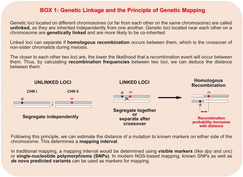
2.2 General steps for identifying a mutation
Identifying a phenotype-inducing mutation requires mapping it to a chromosomal region via genetic linkage analysis and pinpointing the causal variant. The general steps involved in the process are:
Performing a mapping cross: A mutant strain is crossed with a mapping strain, a strain that contains genetic markers or polymorphic loci that distinguish it from the mutant strain. Heterozygous F1 progeny from a mapping cross give rise to F2 recombinants, which are selected based on their mutant phenotype and analyzed.
Determining a mapping region: A chromosomal region that contains the mutation of interest is defined. This is achieved by estimating the distance of genetic markers or polymorphic loci relative to the mutation, from the analysis of recombination frequencies in the F2. Mapping provides intervals with distinct physical boundaries (the actual locations of the markers used for mapping) as well as probabilistic intervals, through distance estimates.
Identifying the causal mutation or “cloning the gene”: This step involves compiling a list of candidate genes/mutations within the mapping region and determining which of them is responsible for the phenotype through phenocopy, complementation tests, and rescue experiments.
3. Traditional Positional Cloning Methods
3.1 Traditional mapping methods
Traditionally, mapping a mutation was a multistep process, where gross and fine mapping were performed successively. It included multiple rounds of crossing followed by the analysis of individual recombinants. A mutation was mapped using visible genetic markers such as Dumpy (dpy) or Uncoordinated (unc) mutations. Mapping against markers on each of the six chromosomes (linkage groups) placed a mutation within a large chromosomal region, a process known as “two-point mapping” (Fay 2013). Mapping against two linked markers that flank the mutation, known as “three-point mapping,” achieved a finer mapping interval (Fay 2013). When the C. elegans genome was sequenced (C. elegans Sequencing Consortium 1998), it became possible to perform genetic mapping using single-nucleotide polymorphisms (SNPs) identified in wild isolates (Koch et al. 2000). The subsequent identification of >100,000 SNPs between the reference C. elegans Bristol N2 and Hawaiian CB4856 (HA) strains was instrumental in improving the efficiency and resolution of genetic mapping (Wicks et al. 2001). These polymorphisms were initially detected using polymerase chain reaction (PCR) combined with Sanger sequencing or restriction enzyme analysis. Advances in SNP detection technologies (reviewed in Davis and Hammarlund 2006) allowed the analysis of pooled samples to be used, known as “bulked segregant analysis” (Michelmore et al. 1991; Wicks et al. 2001), thereby improving the efficiency of the SNP mapping process. Despite these advances, fine mapping still depended on acquiring and individually analyzing a high number of recombinants. It therefore took several weeks or months of work to obtain a fine-mapping interval.
3.2 Traditional methods for identifying the causal mutation
Even after a mapping interval had been defined, a considerable amount of work remained until the phenotype-causing mutation could be identified. All genes in a mapping region were, in principle, candidates. The downstream process for eliminating all but one candidate included transformational rescue with pools of cosmids or fosmids, which contain parts of the genomic sequence within the mapping region. This was followed by single-cosmid rescue and finally single-gene rescue. Phenocopy with RNA interference (RNAi) or known alleles for the candidate genes and complementation tests could also reveal the gene responsible for the phenotype. Once the gene had been identified, Sanger sequencing of the locus was required to determine the molecular identity of the mutation. Identifying the causal mutation downstream of traditional mapping could take from weeks to months, depending on how broad the mapping region was and how easy it was to rescue the phenotype.
4. Mapping-by-Sequencing
4.1 General principles
The use of NGS-based approaches to simultaneously map and identify all genetic variations in the genome of a mutant strain has revolutionized positional cloning (Lister et al. 2009; Hobert 2010), dramatically reducing the time it takes to identify a causal mutation. Although whole-genome sequencing (WGS) determines all sequence differences that distinguish a mutant strain from the reference genome, mapping information is still required, since mutant strains contain multiple genetic alterations originating from natural background variation or the mutagenic treatment itself. Thus, WGS of mutant strains was initially used in combination with traditional mapping (Sarin et al. 2008; Flowers et al. 2010). Far more powerful is the ability to map the causal variant simultaneously with its identification, through WGS of recombinant animals following a mapping cross. This is known as mapping-by-sequencing.
Mapping-by-sequencing was introduced in Arabidopsis thaliana (Schneeberger et al. 2009) and rapidly adopted in C. elegans (Doitsidou et al. 2010; Zuryn et al. 2010). It has since proven to be a rapid, cost-effective strategy in a wide variety of organisms (reviewed in Hobert 2010; Schneeberger and Weigel 2011; Zuryn and Jarriault 2013; Schneeberger 2014). As with all genetic mapping approaches, mapping-by-sequencing relies on the principles of genetic linkage (Box 1). The key difference compared with the traditional mapping methods outlined earlier (see section 3) is that rather than assessing linkage through laborious analysis of individual markers, linkage is assessed by probing a multitude of polymorphic loci simultaneously at a genome-wide level, greatly increasing both speed and mapping accuracy.
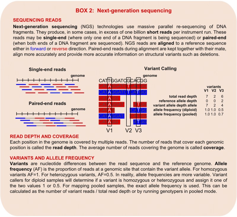
Below we present in more detail each of the mapping-by-sequencing methods in C. elegans. We first consider the most straightforward example involving single-locus recessive mutations and then discuss a series of more challenging cases. We assume a basic understanding of NGS technologies (reviewed in Metzker 2010) and familiarity with related terminology (Box 2).
4.2 Overview of mapping-by-sequencing strategies
Three mapping-by-sequencing strategies have been used in C. elegans that differ in the type of the mapping cross involved (outcross vs. backcross) and how the sample is analyzed. These strategies are:
HA variant mapping, which involves an outcross to a polymorphic strain (typically HA) and genetic linkage analysis of HA SNPs in pooled recombinants (more generally known as bulked segregant analysis) (see section 4.3).
Ethyl methanesulfonate (EMS)-density mapping, which involves serial backcrosses and genetic linkage analysis of mutant strain variants in the final backcrossed strain (see section 4.4).
Variant discovery mapping (VDM), where a single backcross is combined with bulked segregant genetic linkage analysis of mutant strain variants (see section 4.5).
The general strategy, analysis, and the advantages/disadvantages of each of these three methods are presented below and summarized in Figure 1, Figure 2, and Table 1. Bioinformatics tools for NGS data analysis are discussed in Section 6. The following general experimental workflow is similar in all mapping-by-sequencing approaches:
Decide on a mapping-by-sequencing strategy (Figure 2 and Table 1).
Perform a mapping cross (see sections 4.3–4.5).
Allow F1’s to self-fertilize.
Pick F2 mutant recombinants.
Generate the population to be sequenced (method-specific variations).
Isolate genomic DNA.
Construct sequencing library (can be outsourced).
Perform whole-genome resequencing (can be outsourced).
Align sequencing reads to the reference genome (see section 6).
Call and filter variants (see section 6).
Plot SNP allele frequencies/homozygosity levels to determine the mapping region (see section 6, Figure 2).
Annotate (see section 6) and prioritize variants in the mapping region to identify candidate mutations (see section 5.1, Figure 3).
Pinpoint the causal mutation (see section 5.3).
In analyzing the data, it is important to bear in mind which set of SNPs is useful for mapping and which for identifying candidate alleles, as these differ in the three methods presented. This will ensure that the appropriate analysis steps (variant calling, filtering, and subtraction) are performed and the correct allele frequencies are calculated and plotted.
Figure 1.

Experimental workflow of the three NGS-based methods for mutation mapping and identification. Black worms, mapping strains; red worms, homozygous for the mutation; gray worms, heterozygous. In each step, we refer to the corresponding section in the text, and/or figure or table where the reader can find more detailed information.
Figure 2.

Mapping-by-sequencing methods. An illustration of the sequential steps (1–8) involved in (A) Hawaiian variant mapping, left column; (B) EMS-density mapping, middle column; and (C) Variant discovery mapping, right column. Step 1: A mapping cross is performed; in the case of EMS-density mapping, 3–6 sequential backcrosses are performed. Step 2: Either a pool of recombinants (bulked segregant methods) or the serial backcrossed strain is whole-genome sequenced. Step 3: Variants in the background strain (green diamonds) are subtracted. This is not needed for HA mapping as it uses a published set of predefined variants found in the Hawaiian polymorphic strain. Step 4: The subtraction of the background leaves only EMS-induced variants for mapping (red diamonds). In HA variant mapping, a predefined list of SNPs is used (yellow diamonds). Step 5: Allele frequencies of the mapping variants are plotted, revealing the linked mapping region. The green dotted line indicates that in the absence of background subtraction, no mapping region would be identified. Step 6: The background variants are now subtracted in the Hawaiian mapping method. This leaves only EMS-induced mutations. Step 7: Candidate mutations are those variants that remain within the mapping region after background (and other mutant strains) subtractions. Step 8: Candidate variants are annotated and prioritized based on the changes they induce (in this example stop > missense > intergenic. This is indicated in shades of gray). For more details on how to identify the causal mutation (large red diamond) downstream of mapping, see Figure 3.
Table 1. Comparison of mapping-by-sequencing methodologies.
| Outcross | Backcross | ||
|---|---|---|---|
| Bulked (HA mapping) | Serial (EMS density) | Bulked (VDM) | |
| Principle | Mapping interval inferred through segregation of known HA SNPs in pooled F2 recombinants | Mapping interval inferred through increased density of EMS-induced variants after serial backcrosses | Mapping interval inferred through segregation of de novo discovered SNPs in pooled F2 recombinants |
| Cross with | Hawaiian (or other polymorphic strain) | Background nonmutagenized strain (or other available strain) | Background nonmutagenized strain (or other available strain) |
| Step by step | Cross, pool 20–50 F2 homozygous recombinants, WGSa the pool | Backcross 3–6 times, WGSa the backcrossed strain | Cross, pool 20–50 F2 homozygous recombinants, WGSa the pool |
| Variants followed | Variants from mapping strain (HA variants) | Variants from the mutagenized strain (i.e., EMS induced) | Variants from the mutagenized strain (EMS induced only or EMS + background strain variants) |
| Other strains to sequence | Background strain (for variant identification subtraction)b | Mapping strain (for mapping and variant identification subtractions)b | Mapping strain (for mapping and variant identification subtractions)b |
| Mapping plots | HA variant allele frequency | Density of EMS-induced SNPs per physical bin | Mutant variant allele frequency |
| Main advantages | Highest map resolution (>100,000 SNPs) | Mutant strain is already backcrossed after mapping protocol | High mapping resolution |
| Can be used to map the absence of a mutation | Basic genetic tests can be performed during backcrosses | Can be used in all mutation categories | |
| Fast (requires only one cross) | Convenient with complex screening strains | Can be used for mapping the absence of a mutation | |
| Convenient with difficult phenotypes | Fast (requires only one cross) | ||
| Appropriate for species where polymorphic strain unavailable | Basic genetic tests can be performed during backcross | ||
| Appropriate for species where polymorphic strain unavailable | |||
| NOT appropriate for | Phenotypes that might be affected by Hawaiian background | Spontaneous mutations, mutant strains generated without EMS or high density mutations | |
| Complicated background strains (background mutations e.g., modifier screens) | Mapping the absence of a mutation | ||
Followed by standard bioinformatics analysis: Mapping and alignment to reference genome, variant calling and annotation (see Bioinformatics and Pipelines). This can be done with Cloudmap, home-made pipelines, or as part of sequencing service.
Background (or mapping strain) variants can also be obtained by sequencing other mutants from the screen.
Figure 3.

From mapping interval to causal mutation. An illustration of the steps (1–5) involved in going from a mapping interval, defined through a WGS-based approach to identifying the causal variant. Mut, mutation.
4.3 HA variant mapping (bulked segregant analysis after outcrossing)
4.3.1 Concept and mapping cross (HA variant mapping):
This method involves outcrossing to the highly polymorphic CB4856 HA strain followed by WGS (Figure 2A). Conceptually similar to traditional SNP mapping, WGS-based HA variant mapping makes use of the known HA SNPs for mapping but in a much more efficient manner: all ∼105 HA SNP loci are assessed simultaneously for genetic linkage to the causal mutation. In this strategy, homozygous mutant hermaphrodites are crossed with HA males to generate F1’s in which meiotic recombination occurs (in principle, the sexes can be reversed). In the F2 generation, 20–50 homozygous mutant recombinants are selected (Figure 2A). These F2’s are allowed to self-propagate through the F3/F4 generations and are washed off the plate as soon as the plate begins to starve. These worms are then pooled and the pool is whole-genome sequenced (Doitsidou et al. 2010; Minevich et al. 2012).
4.3.2 Analysis method (HA variant mapping):
After whole-genome sequencing of the recombinant pool, bioinformatics analysis, described in more detail in section 6, is performed to align the sequencing reads to the genome and generate the list of variants (or call the variants). In fact, HA variant mapping involves calling variants twice. First, for mapping, a list of all known HA SNP positions is generated and the allele frequencies are calculated. This is done by dividing the number of sequencing reads containing the HA allele by the total number of reads at each HA SNP position. The allele frequencies across each chromosome can then be plotted to reveal the mapping location. The selection of homozygous F2 mutant animals ensures that the linked region will be progressively more and more devoid of HA SNPs the closer one approaches the causal mutation (Figure 2A). The region devoid of HA alleles reveals the mapping interval. Second, a list of all variants in the mutant strain pool is generated. From this list, background variants (present in the starting mutagenesis strain or present in other mutant strains from the same screen) are subtracted, and those remaining in the mapping region are examined as potential causal variants. This analysis can be performed using a prebuilt bioinformatics pipeline in the free, online-based CloudMap platform (Table 2 for links to tutorial) or custom-made pipelines (described in section 6).
Table 2. Useful bioinformatics links.
To improve mapping accuracy, regression analysis [e.g., local regression (LOESS)] can be performed (Minevich et al. 2012). Fitting a regression line through the thousands of data points in the mapping plot, which reflect recombination frequencies along the chromosome, further refines the mapping interval. In other model systems, probabilistic models, such as Bayesian networks (Edwards and Gifford 2012), Hidden Markov models (Leshchiner et al. 2012), likelihood test statistics (Galvão et al. 2012), and G statistics (Magwene et al. 2011), have been used.
It is also possible to calculate and plot the frequency of pure parental N2 alleles (i.e., those with 100% N2 reads) compared to total variants in discrete bins (e.g., 1- or 0.5-Mb bins) across the chromosomes (Minevich et al. 2012). The mapping region corresponds to the bin with the highest frequency of N2 alleles. Genetic incompatibilities between N2 and HA, such as those caused by the peel-1/zeel-1 loci (Seidel et al. 2008), can distort N2/HA allele frequencies owing to the lethality of certain genotypes. The impact of such incompatibilities on binned N2 allele counts can be minimized by simple normalization (multiplying the frequency of pure N2 alleles by the average number of pure N2 alleles per bin, per chromosome) (Minevich et al. 2012). This normalization has the effect of exaggerating the pure N2 frequency only for the most linked chromosome. In other model systems, sliding windows of allele frequencies have been used (Sun and Schneeberger 2015). The CloudMap pipeline automatically generates both LOESS and binned plots of pure N2 allele frequency (see section 6 and Table 2 for links to tutorials).
4.3.3 Advantages/disadvantages (HA variant mapping):
The major advantage of this method is the high mapping accuracy that is achieved owing to the simultaneous analysis of the large number of known defined HA SNPs (>100,000; density of 1/1000 bp) (Table 1). Furthermore, mapping resolution is increased by statistical extrapolation, such as LOESS regression, which gives probabilistic mapping intervals that are narrower than just the physical boundaries of the closest recombination event. In addition, HA variant mapping is fast to implement, as it requires only one cross. The main disadvantages are that, in C. elegans, certain phenotypes may be affected by the HA background. In addition, this method is not optimal for complicated mutant strains with background mutations (or reporters) that need to be kept homozygous during a mapping cross (for example in modifier screens). The HA variant mapping method has been successfully used to identify the causal variant in a variety of mutant strains (Doitsidou et al. 2010; Labed et al. 2012; Minevich et al. 2012; Liau et al. 2013; Connolly et al. 2014; Wang et al. 2014; Jaramillo-Lambert et al. 2015; Smith et al. 2016).
4.4 EMS-density mapping (mapping after serial backcrossing)
4.4.1 Concept and mapping cross (EMS-density mapping):
This method involves serial near-isogenic backcrossing of the mutant strain (e.g., to the nonmutagenized starting strain) and the assessment of genetic linkage of variants predicted de novo from the whole-genome sequencing data for mapping (Figure 2B). The mapping interval in this method is defined by the chromosomal recombination boundaries rather than statistical extrapolation, since serially backcrossed samples (unlike pooled recombinant samples) do not carry information on recombination frequencies (Zuryn and Jarriault 2013). The causal variant is identified from the same list of variants used for mapping. After each backcross, a recombinant mutant F2 animal is picked and backcrossed again. Following at least three rounds of serial backcrossings (and optimally four to six), the DNA from the backcrossed homozygous mutant strain is prepared and sent for WGS. This method has also been called EMS-based mapping (Zuryn et al. 2010).
4.4.2 Analysis methodology (EMS-density mapping):
Serial backcrossing removes EMS-induced SNPs that are not linked to the causal variant, leaving a linked region enriched for homozygous EMS-induced mutations. To reveal the mapping region, first all variants present in the serially backcrossed strain are identified. Then background variants common between the mutant strain and the backcrossing strain need to be subtracted (Figure 2B). The background variants can be obtained from other mutant strains from the same screen or by sequencing the nonmutagenized starting strain. The remaining variants are filtered for homozygous, EMS-typical mutations (G:C to A:T transitions) and the density of these variants is plotted to reveal the mapping region. The same list of background-subtracted variants can then be used to identify the causal variant within the mapping the region. It is worth noting that these may or may not be canonical EMS-induced variants, and so it is worth examining all variants, including those that are not G:C to A:T transitions. Given the lower density of EMS-induced SNPs (compared with HA SNPs), it is important to ensure a high coverage and stringent variant filtering for the SNPs used to generate the mapping plots (see section 6). The CloudMap pipeline can perform all this analysis in one go (see Table 2 for links to the EMS-density mapping-specific pipeline).
It has been calculated that increasing the number of backcrosses beyond six, used in Zuryn et al. (2010), will not significantly improve the mapping accuracy. However, the mapping accuracy can be improved by pooling two or three serially backcrossed versions of the mutant strain (James et al. 2013). Notably, performing serial outcrosses rather than backcrosses is also possible, provided that the variants in the outcrossing strain are also analyzed by WGS and subtracted.
4.4.3 Advantages/disadvantages (EMS-density mapping):
Given that the mapping cross is to any strain of choice, usually the starting strain, the advantages of this method are that it can also be used when complicated genetic backgrounds are involved or if the phenotype is altered in a polymorphic strain background (such as HA; Table 1). An added benefit is that by the end of the EMS-density mapping protocol, the mutant strain has already been backcrossed a few times and is ready for experiments, and basic genetic tests have been concomitantly implemented. Finally, as very few recombinant animals need to be recovered for the serial backcrossing, this method is particularly suited to when F2 mutant animals are not easily identifiable, recoverable, or have a very low penetrance. The main disadvantage of EMS-density mapping is lower mapping resolution owing to the lower density of EMS-induced SNPs and the inability to use allele frequencies across the chromosome for refining the mapping region. EMS-density mapping has successfully been used to clone numerous mutants (Zuryn et al. 2010, 2014; Svensk et al. 2013; Neumann and Hilliard 2014; Steciuk et al. 2014; Tocchini et al. 2014; Rauthan et al. 2015).
4.5 Variant discovery mapping (bulked segregant mapping after a backcross)
4.5.1 Concept and mapping cross (VDM):
VDM combines principles from both previous methods (Minevich et al. 2012). As with EMS-density mapping, a near-isogenic backcross is performed between the mutant and the nonmutagenized starting strain. However, instead of serial backcrosses, VDM uses a bulked segregant analysis approach, similar to the HA variant mapping method. Specifically, several homozygous F2 mutant recombinants are selected and allowed to self-propagate through F3/F4’s, then pooled, and their DNA is isolated and prepared for whole-genome sequencing (Figure 2C). A list of de novo predicted variants in the mutant pool is then used both for mapping and causal variant identification. Here the mapping interval is defined by both recombination break points and recombination frequencies.
4.5.2 Analysis methodology (VDM):
In VDM after WGS, all SNPs present in the F2 pool of homozygous mutant recombinants are identified de novo from the WGS data set. Background variants present in the nonmutagenized starting strain are then subtracted, leaving the unique mutagen-induced SNPs required for mapping (Figure 2C). As with HA variant mapping, the allele frequencies of these SNPs are then calculated and plotted on a graph to reveal the mapping region. The selection of homozygous F2 mutant animals ensures that within the pool, unlinked SNPs have an allele frequency of 0.5, but this progressively increases toward an allele frequency of 1.0 the closer one approaches the causal mutation (Figure 2C). LOESS regression analysis can again be used to reveal the trend in the data and further refine the mapping region (Figure 2C) (Minevich et al. 2012). Binned frequency plots of alleles with a frequency of 1.0 can also be used. Again, the CloudMap pipeline has automated workflows that produce both of these plots (see section 6 and Table 2 for links to tutorials).
It is possible to use this method following an outcross (rather than a backcross) to a strain other than the starting strain, as long as the SNPs/indels present in the outcrossing strain are known. These will need to be subtracted from the de novo predicted SNPs/indels in the recombinant pool so that only SNPs from the mutant parental strain are followed. Following SNP alleles from one parent at a time is crucial because the allele frequencies of SNPs present in each parental strain move in opposite directions in the pool of mutant recombinants (compare mapping plots in Figure 2, A–C). VDM by outcrossing actually allows the use not only of mutagen-induced SNPs for mapping but also of any SNPs present in the background of the mutant strain, improving mapping accuracy (Minevich et al. 2012).
4.5.3 Advantages/disadvantages (VDM):
VDM combines some of the advantages of the mapping methods described above. First, as in EMS-density mapping, any mapping strain of choice can be used. By using the nonmutagenized starting strain to perform the mapping cross, VDM allows mapping of mutations in strains with complicated genetic backgrounds or mutations with phenotypes that are altered by a polymorphic strain, and the single cross can be used to concomitantly implement basic genetic tests. Second, as in the HA variant mapping method, the mapping interval is not bounded by the recombination break points nearest to the mutation. Rather, by assessing recombination frequencies across the chromosome, these methods enable a confidence interval within the recombination break points to be mathematically assigned, increasing mapping accuracy. The primary disadvantage of VDM, just as with EMS-density mapping, is the low density of mutagen-induced SNPs, which limits mapping accuracy. As mentioned in the previous section, this can be mitigated to a degree by using an outcross achieving higher mapping accuracy, although not as high as in HA variant mapping. The VDM method has recently been successfully applied to the identification of mutants affecting the innate immune response in C. elegans (Cheesman et al. 2016).
4.6 Practical considerations
The most important variables that affect mapping resolution are the numbers of recombinants, the sequencing depth, and the density and quality of variants. In all cases, the higher these variables are, the better the mapping resolution, with increases in the numbers of recombinants having the largest effects (James et al. 2013). When choosing a bulked segregant approach, we therefore strongly recommend the collection of as many recombinants as possible. We find that ∼50 is ideal to ensure mapping to an 0.5-Mb region, but as few as 10 recombinants give mapping intervals with a manageable number of variants.
As for the sequencing itself, a variety of NGS platforms exist and are commercially available (reviewed in Mardis 2013). The Illumina platforms (such as the NextSeq and HiSeq systems) are currently the most readily available and the most broadly used by institutional and commercial services. They have been shown to have high throughput and accuracy, and a comparatively low cost per megabase. For the NGS novice, we recommend genomic DNA isolation using standard protocols or kits (we particularly like the Gentra Puregene Kit (QIAGEN, Valencia, CA). Careful washing should be performed to ensure that bacteria are removed; the presence of bacterial DNA or RNA from the lysed worms will reduce sample coverage, since a portion of the sequenced reads will be of bacterial origin. The library preparation is usually outsourced to the sequencing provider. This step, which typically involves fragmenting the DNA, ligating the adapters, and performing a few rounds of PCR amplification is critical, and the protocols are specific to the sequencing platform used. Although it is relatively straightforward, the plummeting costs of NGS leave little financial gain from performing library preparation in the laboratory. Both paired-end and single-end reads can be used (Box 2). However, paired-end sequencing has the advantage that structural variations can also be analyzed (see section 6.3). It has also been suggested that paired-end sequencing produces a higher number of informative reads owing to improved mapping quality. The choice of read length is not as crucial and can be influenced by the standard procedure of the in-house facility or the sequencing service used. It is worth keeping in mind that although longer reads map more accurately, they have lower sequencing quality at the ends compared to shorter reads. Finally, we recommend sequencing to a minimum coverage of 20–30× for better mapping accuracy, as higher coverage allows calling of low frequency alleles in pooled samples more confidently. Adequate calling of homozygous variants can occur with 10–15× coverage (Bentley et al. 2008). However for heterozygous variants, a coverage of >30× is recommended (Bentley et al. 2008) and of at least 60× for structural variants (SVs) (e.g., deletions, insertions, inversions, etc.) (Fang et al. 2014).
4.7 Mapping special case mutations
With very few exceptions, the mapping strategies discussed above can be adapted to virtually any mutant category. The success of a mapping protocol depends on distinguishing F1 cross-progeny and confidently isolating homozygous recombinant F2 mutant animals. Setting up mapping crosses and picking recombinants is simpler when dealing with single recessive loci that give highly penetrant obvious phenotypes. However, we often have to deal with more challenging mutations; therefore, careful planning of a mapping cross is essential. Below we will discuss some categories of challenging mutations and how the above mapping-by-sequencing protocols can be adjusted to accommodate such cases.
4.7.1 Dominant mutations:
Any of the mapping methods described above can be used, with some adjustments, for dominant mutations. Caution is required at some points during the mapping cross, however. First, with dominant mutations heterozygous animals cannot be readily distinguished from homozygous animals based on phenotype. Therefore, if the mapping strain does not contain a visible marker, F1’s can be blindly picked from a successful cross-plate and the phenotypic segregation in the F2 can be used to distinguish self- from cross-progeny F1’s. Similarly, when picking F2 recombinants, an extra generation should be allowed to assess homozygosity by looking at the F3 progeny (Smith et al. 2016), a practice recommended for recessive mutations, too, as any contamination of the pool with heterozygous samples will affect the mapping accuracy (Doitsidou et al. 2010). With these considerations in mind, mapping viable dominant mutations with WGS can follow any of the strategies described above and their corresponding data processing pipelines.
It is also possible to map the absence of the mutation (reverse mapping). In this case, F2 recombinants without the mutant phenotype are selected and their progeny are pooled to generate the mapping population (Smith et al. 2016). The pool is then sequenced to generate mapping information. An additional WGS reaction (of the homozygous mutant) is required to identify the actual mutation. Reverse mapping, despite the additional cost, is the preferred method for mapping dominant mutations in cases when assessing the F3 phenotype is not possible; for example, in cases of F2 lethality, sterility, or maternal-effect lethal phenotypes. As the name of the method implies, in reverse mapping the appearance of the mapping plots will be reversed: For example, with HA mapping, the plotted ratios of HA SNPs rises to 100% in the mapping interval. A proof of principle of this approach has been provided (Smith et al. 2016). Conversely, when using reverse VDM, the ratios of parental alleles are zero within the mapping region. An alternative strategy has been demonstrated that depends on backcrossing twice to the nonmutagenized starting strain and then selecting heterozygous mutant animals with the dominant phenotype for sequencing (Lindner et al. 2012). Allele frequency will be 0.5 for linked alleles, and 0.25 for unlinked alleles, and this can be detected by plotting allele frequencies.
The same principles can be followed for semidominant alleles. In cases where the intermediate heterozygous phenotype is clearly distinguishable from the homozygous mutant and the wild type, semidominant alleles can be processed following a strategy similar to that for recessive mutations.
4.7.2 Lethal, developmental arrest and sterile phenotypes:
In the case of terminal phenotypes, which include larval lethality, developmental arrest, or sterility, it is not possible to amplify the homozygous mutant recombinant animals unless the allele is temperature sensitive (Jaramillo-Lambert et al. 2015). The challenge therefore is to acquire enough material from individually picked F2 recombinants for whole-genome sequencing. Although standard library preparation kits require micrograms of genomic DNA as starting material, kits have been developed that are appropriate for low amounts of starting material and genomic DNA on the order of nanograms. In a proof-of-principle study, it has been shown that significant library bias is not introduced when starting with low genome DNA input, and comparable mapping and variant detection results were obtained (Smith et al. 2016); 50 hand-picked sterile F2 recombinants yielded enough DNA for library construction. If it is possible to directly identify heterozygous F2 animals unambiguously or by assessing F3 phenotypes, then the double backcross method mentioned above (see previous section 4.7.1) could in principle also be used (Lindner et al. 2012).
Embryonic lethal mutations are best dealt with by designing screens that target their isolation, e.g., using balancer strains (Edgley et al. 2006). Lethal mutations can then be mapped following EMS-density mapping or VDM using the balancer strain as the backcrossing strain, and hand-picking dead F2 embryos/larvae for sequencing. Although the HA variant mapping method has been successfully used to map embryonic lethal mutations (Jaramillo-Lambert et al. 2015), caution is required as genetic incompatibilities between the N2 and HA strains may confound the retrieval of dead homozygous embryos (Seidel et al. 2008). Pipelines for WGS data have also been developed that integrate allele ratio and information on the mutational landscape to analyze heterozygous SNPs in balanced lethal mutant strains (Chu et al. 2012). Such approaches have been successfully used to identify the molecular lesion in several lethal strains (Chu et al. 2014).
4.7.3 Low-penetrant mutations and subtle phenotypes:
When mapping low-penetrant mutations or subtle phenotypes, careful quantification is required to assess homozygosity in the F2 generation. The lower the penetrance of a phenotype, the more F1’s are needed to obtain the desirable number of homozygous F2 mutant recombinants. While most strategies described above are appropriate for low-penetrant mutations, strategies requiring a very small number of recombinant F2’s, like EMS-density mapping, are easier to implement. Reverse mapping is not recommended for low-penetrant recessive mutations, as it is easy to miss low occurrence phenotypes in heterozygous populations and inadvertently contaminate the pool of recombinants with heterozygous animals.
4.7.4 Synthetic phenotypes (multi-loci mutations):
Synthetic (or multiloci) mutations can be mapped in a similar manner to single-locus mutations, choosing any of the three main strategies described earlier. The only difference is that in the F2 generation, the proportion of double homozygous mutant animals will be significantly lower (1/16) and thus it might be easier to start with a higher number of F1 cross-progeny to obtain the desirable number of F2 double-mutant recombinants (similarly to phenotypes with incomplete penetrance, partial lethality, or slow growth). The ensuing mapping plots will inevitably show linkage with all loci required for the phenotype. In fact, although it is helpful to have prior knowledge that a mutant phenotype depends on more than one locus, it is not necessary, as this will be clearly revealed by the mapping result. A proof of principle of HA mapping of a two-loci mutant was reported (Smith et al. 2016). Caution is needed in cases of synthetic mutations where each of the individual mutations also has a detectable phenotype. In such cases, the pool of recombinants might be “contaminated” with mutant animals homozygous for one of the loci but heterozygous for the other and vice versa.
4.7.5 Modifier mutations:
Modifier screens are often used to identify secondary mutations that alter a known mutant phenotype. To map modifier mutations, the original mutation needs to remain in the background during the mapping process. Thus, for convenience, we recommend using the nonmutagenized starting strain as the mapping strain and performing either EMS-density or VDM with de novo predicted SNPs (see sections 4.4 and 4.5). Using the background strain as the mapping strain ensures that the original mutation, whose phenotype is being modified, remains homozygous during the mapping cross, avoiding additional linkage points. The result is a single clear mapping region. Similarly, in male screens performed in him backgrounds, a backcrossing strategy with the him background strain can be used to increase the number of F2 males available for observation. It is also possible to use HA variant mapping if the original mutation is introduced in the HA strain (ideally engineered by the clustered regularly interspersed palindromic repeats (CRISPR)-Cas9 system rather than introgressed), contingent on the HA strain showing the same phenotype for the original mutation. This approach has been successfully implemented for identifying suppressors of mbk-2/DYRK (Wang et al. 2014). To our knowledge this has not yet been done for him mutations, but this would be an excellent solution to allow Hawaiian bulked segregant analysis of male phenotypes.
4.7.6 Maternal-effect mutations:
Maternal-effect mutations show no phenotype as homozygous progeny of a heterozygous parent owing to maternal contribution of the wild-type gene product. There are two categories of maternal-effect mutations: lethal and nonlethal. Lethal maternal-effect mutations are viable as homozygous animals produced from heterozygous mothers, but give rise to dead F3 progeny. This category can therefore be treated similarly to sterile phenotypes (see section 4.7.2) (Jaramillo-Lambert et al. 2015). For viable maternal-effect mutations (Hekimi et al. 1995), any mapping-by-sequencing methodology can be applied. However, when assessing homozygosity of recombinants after a mapping cross, an extra generation should be allowed (F3) to confirm that the mutation is indeed homozygous.
4.8 How much genetic analysis before mapping?
As seen in the previous sections, the various mapping-by-sequencing strategies can be adjusted, depending on the mutant phenotype and the type of alleles retrieved. A question often asked concerns how much genetic analysis should be done prior to mapping? We recommend a quick backcross with the nonmutagenized strain or the reference N2 to perform genetic diagnostics (to determine whether the mutation is recessive or dominant, affects a single locus or multiple loci, or is linked to chromosome X). In VDM or EMS-density mapping, the required genetic information can be directly extracted from the mapping cross itself. As some incompatibilities leading to lethality or alteration of the phenotype have been described when N2-based and HA strains are crossed (Seidel et al. 2008; Neal et al. 2016), the use of the CB4856 strain to conduct these genetic tests is best avoided. Overall, a time-saving recommendation is to proceed with the mapping cross immediately after mutant isolation and to perform the basic genetic analysis of the mutant either in parallel or, when possible, through the mapping cross itself. In any case, it is important to remember that backcrossing a mutant is necessary for proper downstream phenotypic analysis.
5. Identifying the Causal Mutation
This section deals with identifying the causal variant after a mapping region has been defined. As with the mapping section above, the following section primarily deals with the principles driving the analysis. The majority of the filtering and subtraction steps described below can be performed in a relatively straightforward manner using the bioinformatics pipelines that are discussed in section 6. Besides the variant subtraction steps that are part of the mapping workflows, CloudMap also offers a separate workflow dedicated to subtracting variant data sets (Table 2).
5.1 Narrowing down the candidate list: subtractions and filtering
In mapping-by-sequencing protocols, a single sequencing step reveals not only the mapping region but also all of the mutations in the sequenced sample. How do we go from a mapping interval and a list of variants to finding the phenotype-causing mutation? A number of subtraction and filtering steps can be performed to eliminate many of the variants (Figure 3). A first step for narrowing down the list of variants obtained by WGS is to subtract all background strain variations (homozygous and heterozygous) from the list of variants identified in the mutant strain. It is thus useful to sequence the background strain at a satisfactory depth to ensure that the majority of background variants will be discovered. It is also useful to subtract common variants identified in other mutant strains from the same screen, as long as they map to a different interval than the mutant under investigation.
Once subtractions are complete, filtering criteria can be applied to further narrow down the list of candidates. First, it is important to select only homozygous variants within the mapping region (assuming that the sample sequenced is homozygous for the mutation). Filtering based on quality or sequencing depth should not be very stringent at this stage to ensure that the phenotype-causing mutation is not inadvertently removed. When the sequenced sample is not homozygous for the mutation, filtering variants by allele frequency should be adjusted accordingly.
Next, prioritize the most likely type of mutations, depending on the mutagenic agent, e.g., in the case that EMS is used as the mutagen, the most frequently occurring mutations, G-to-A and C-to-T transitions, could be considered first (although atypical mutations occasionally occur and should not be completely discounted). Priority should be given to variations that have an obvious effect on the gene product, e.g., nonsense, missense, splice-site SNPs, and structural variations (like insertions, deletions, inversions, etc.) that affect coding regions. If no obvious candidates exist among the protein-changing SNPs, then regulatory promoter or intronic mutations within the mapping region should be considered. Checking the degree of conservation across genomes from different species around putative mutations on the University of California Santa Cruz genome browser (http://www.genome.ucsc.edu) can provide additional prioritization criteria for variants that do not obviously affect an open reading frame (Zuryn and Jarriault 2013). Once a list of candidate mutations in the mapping region has been compiled, a quick Sanger sequencing might be warranted (depending on the depth and quality of reads) to confirm the presence of the candidate variant in the mutant and its absence from the background strain. The confirmed list of variants is then considered for downstream processing to identify the causal mutation.
5.2 In silico complementation
In silico complementation is a powerful method to determine whether multiple alleles of the same gene exist in a collection of sequenced mutant strains. It is particularly useful in cases when multiple mutants from a screen map to the same interval. In such cases it can directly pinpoint the phenotype-causing gene (Nagarajan et al. 2014). A bioinformatics module for in silico complementation is present in the CloudMap pipeline (see section 6) (Minevich et al. 2012). In silico complementation provides an unbiased approach for identifying allelic mutations because it is informed by the actual presence of variations at a given locus and is supported at the same time by mapping data. It is therefore devoid of the genetic bias that classic complementation experiments can introduce, for example in cases of nonallelic noncomplementation (when two mutations affecting different genes fail to complement each other) or allelic complementation (when two alleles affecting the same gene complement each other).
5.3 Pinpointing the causal mutation
After subtractions, filtering, and performing in silico complementation, a successful mapping experiment usually results in a small list of candidate variants that should be easy to validate experimentally (Figure 3). How can we pinpoint the phenotype-causing mutation among a list of candidates? Strategies largely depend on the genetic properties of the mutation. For recessive mutations, standard validation practices include complementation with available alleles, reproducing the phenotype with RNAi and/or known alleles of the gene, and transformational rescue. For dominant mutations, however, confirming the causal mutation is not as straightforward because rescue with the wild-type copy is often not feasible. In addition, dominant mutations can fall into various categories (detailed in Fay 2013), each one of which may give different results using the same genetic tests. For example, when a mutation causes a dominant phenotype due to haploinsufficiency (a situation when one wild-type copy is not enough to provide the wild-type function), strategies like transformational rescue or phenocopy with RNAi can give an informative result. In contrast, the same strategies will give negative results in the case of a gain-of-function dominant mutation. In situations where loss-of-function of the same gene has no detectable phenotype, gain-of-function mutations can be validated by knocking down the identified gene in the mutant strain to rescue the phenotype. A more universal strategy for proving causality for dominant mutations is attempting to recapitulate the phenotype by introducing the mutated candidate locus into the wild-type background.
A simple strategy to irrefutably prove that a mutation is indeed causal to a phenotype is to use CRISPR-Cas9 genome editing to introduce the exact same mutation in the wild-type strain (Dickinson and Goldstein 2016). CRISPR-Cas9 genome editing can be applied for any type of mutation, dominant or recessive, loss or gain of function, open reading frame (ORF) affecting, or regulatory, etc., which makes it particularly valuable as a confirmation strategy in cases when the standard genetic methods cannot be used. As CRISPR-Cas9 genome editing protocols become more efficient and easy, it is fair to assume that introducing candidate mutations into wild-type backgrounds may soon be the preferred method of pinpointing the causal variant from a list of few candidates.
6. Bioinformatics and Pipelines
Perhaps the biggest challenge for the novice in mapping-by-sequencing is the bioinformatics processing of NGS data. A basic workflow for mapping-by-sequencing consists of the following main steps:
Alignment of sequencing reads to the reference genome.
Variant calling.
Variant filtering/subtraction.
Calculation/plotting of allele frequencies.
Variant annotation.
In addition to the continued development of the specific tools that perform these functions, over the past few years a number of online data analysis platforms have been developed. These platforms simplify the execution of the above steps by providing a user-friendly interface that groups bioinformatics tools together in pipelines to facilitate analysis. In this section, we first highlight the Galaxy data analysis platform and then we introduce the Cloudmap and MiModD pipelines. We touch briefly upon the use of commercial services and then outline a more detailed workflow for those readers wishing to understand the key concepts of the individual steps involved (Figure 4). In Table 2, we provide a list of useful links to pipelines, the Galaxy platform, descriptions of file formats, and a nonexhaustive but illustrative list of bioinformatics tools that collectively consist of a complete workflow for analysis of the WGS data.
Figure 4.

A typical mapping-by-sequencing data analysis workflow. Schematic representation of the bioinformatics analysis steps (1–8) involved in analyzing the NGS data obtained from a mapping strain or population starting from raw FastQ files until a mapping interval and a candidate mutations list is generated. The file format is indicated for each step of the workflow. See Table 2 for links to the bioinformatics tools (FastQC, Sickle, BWA, Samtools, GATK suite, Picard, CloudMap, and SnpEff). Variant metrics or annotation are exemplified for steps 4–6, and 8. V1, V2, and V3 are variants. AF, allele frequency; DP, read depth; Dups, duplicates. For definitions of variant metrics, see Box 2.
6.1 Galaxy and available pipelines
Users with experience in computing can attempt NGS analysis by directly using the bioinformatics tools described in the workflow below (section 6.2) run in the Linux command line. However, we strongly urge novice users without any command-line computing experience to use the available user-friendly pipelines. These pipelines accept FASTQ files, the file type produced from Illumina sequencing (Table 2), implement prebuilt workflows of bioinformatics tools, and produce as an output mapping plots and annotated lists of variants. Several of these pipelines make use of the Galaxy interface (Blankenberg et al. 2010), which is a free, web-based, user-friendly platform for easy management and running of bioinformatics tools, without any advanced computing knowledge. Developed at Penn State University, it can be easily accessed through their public server at https://usegalaxy.org (Table 2). Pipelines designed specifically for C. elegans include:
CloudMap (Minevich et al. 2012) (https://usegalaxy.org/cloudmap).
MiModD (http://www.celegans.de/en/mimodd).
Other pipelines designed for other model systems include:
SNPtrack for zebrafish and mouse (Leshchiner et al. 2012).
SHOREmap for A. thaliana (Sun and Schneeberger 2015).
MegaMapper for zebrafish (Obholzer et al. 2012).
CloudMap is Galaxy-based, whereas MiModD has its own web interface. Importantly, there are comprehensive user guides for both pipelines that explain how to use the web interfaces and run the prebuilt workflows in a point-and-click manner (Table 2). We strongly recommend careful reading of these user guides, in addition to understanding the main concepts described earlier in this review. Both CloudMap and MiModD offer automated workflows for the three main mapping-by-sequencing methods described earlier (see section 4) and can be run on publically available servers, obviating the need for any local install, computing resources, or advanced bioinformatics skills. These automated workflows map reads to the genome, call, and filter variants (both for mapping and identification of the causal variant), and produce allele frequency mapping plots and annotated lists of candidate causal variants. On the Galaxy main public server (Table 2), the CloudMap workflows are called “Hawaiian Variant Mapping,” “Variant Discovery Mapping,” and “EMS Variant Density Mapping.” We note that the CloudMap workflows also incorporate a number of additional tools to analyze possible deletions (see section 6.3) and to perform in silico complementation (Minevich et al. 2012).
In addition to these pipelines, many sequencing facilities (both institutional and commercial) offer standard bioinformatics processing (which does not include mapping plots) and provide annotated variants lists. These variant lists are normally provided in the form of a variant call format (VCF) file (Table 2). As VCF files include read depths for the variant alleles, it is possible to simply calculate and plot allele frequencies (number of variant reads/total reads) for each variant to produce mapping plots. Filtering and subtractions required prior to mapping (see section 6.2) to extract specific sets of variants (for example HA variants if HA mapping is being performed, or EMS-induced variants if EMS-density mapping or VDM is being performed) can be achieved using standard computer software capable of comparing data sets or filtering tables (like Excel).
6.2 Detailed workflow and underlying tools
Although the above pipelines are excellent for the novice user, public servers can be slow and therefore many users, particularly if they are mapping and cloning mutations on a regular basis, may wish to take more control over the process. So what are the possible options for this and what are these pipelines actually doing? All of the automated pipelines mentioned above make use of a number of open source bioinformatics tools (listed below) that process NGS data in a stepwise manner. Users with more advanced bioinformatics knowledge or users willing to take a Linux/NGS data processing course can run these tools on a computer cluster using command line. Clusters of this sort may well be available in your institute. A novice user can also choose to run these bioinformatics tools manually in Galaxy, without the need for command-line expertise. The advantage here, compared with employing the prebuilt pipelines mentioned above, is flexibility to generate custom-made workflows according to the needs of each analysis or to modify workflows to use the most up-to-date tools for each step. In addition, many institutes now provide private Galaxy servers that may be faster than the available public servers. Moreover, Galaxy can be easily run in the cloud or even installed locally (Table 2). Importantly, a number of excellent online guides exist for NGS data analysis on the Galaxy platform (e.g., Galaxy NGS 101 tutorial, see Table 2).
Although it is beyond the scope of this review to describe all possible bioinformatics tools that can be used in each step of analysis and their advantages/disadvantages, it is important that users have a conceptual understanding of the steps involved. We describe next a typical NGS data analysis workflow (Figure 4) for mapping-by-sequencing and provide an example tool (and settings where appropriate) that can be used at each step. Links to downloading these tools and descriptions of file types can be found in Table 2.
Quality control: A single run of a sequencer will produce tens of millions of short reads per sample, which are usually supplied in FASTQ format. In addition to the reads themselves, this file also contains Phred-based quality scores for each nucleotide (Table 2). This quality score is a measure of how likely the correct base has been called by the sequencer. The first step therefore is to assess the quality of your reads using a tool such as FastQC (Table 2). This tool outputs graphs of quality scores, which can be used to assess your input data. It is advisable to use reads that have an average quality score of ≥20. Poor quality reads can be trimmed using a tool such as Sickle (Table 2).
Aligning to the reference genome: The next step is to align the short reads to the genome. The two most commonly used tools are Burrows-Wheeler Aligner (BWA) (Li and Durbin 2010) and Bowtie2 (Ben Langmead and Salzberg 2012). Their input is the quality-controlled FASTQ file and their output is aligned reads in SAM format. This output can then be converted to BAM format using Samtools (Li et al. 2009). BAM files contain not only mapping coordinates for each read but also a Phred-based mapping quality score that represents the confidence that the read was mapped to the correct position. These confidence scores are used when calling variants (see below).
-
Realigning around indels and removing duplicates: Genome aligners can have difficulties aligning reads that contain small indels: since each read is aligned independently, aligners often misalign reads with indels, generating false-positive SNPs and miscalling indel boundaries. The GATK suite of tools allows identification of suspicious intervals where alignment might be inaccurate and performs local realignment using the GATK indel realigner tool (DePristo et al. 2011). These realignment steps are not required for genotype callers that perform realignment automatically during calling, such as GATK HaplotypeCaller or Freebayes.
NGS experiments can generate duplicate reads, which are reads that derive from the same fragment of input DNA. Duplicates occur as a consequence of sample amplification or clustering methods used by Illumina sequencing technology. It is recommended that duplicate reads are removed (or marked) to avoid artificially inflated coverage or allele frequencies that could affect further analysis. Marking of duplicates can be performed using a tool such as Picard (Table 2). This tool looks for reads whose mapping positions and sequence are identical and marks them as duplicates, while leaving only the read with the highest quality unmarked, allowing downstream analysis tools (like GATK) to exclude duplicates from analysis.
Variant calling: Once the reads have been aligned to the genome, variants can be called from the BAM file using one of the various available genotypers such as GATK Unified Genotyper, GATK Haplotype Caller, or Freebayes (Table 2). The public CloudMap pipeline still uses GATK Unified Genotyper as currently only VCF files from this genotyper work well with the CloudMap plotting tools. When using GATK Unified Genotyper, it is recommended that for high coverage (30–60×), high-quality (all reads have Phred-based quality scores of >30 for each base pair according to FastQC) data sets, only reads with a Phred-based mapping score of >30 (1/1000 chance of being mismapped) are used for calling variants. GATK Unified Genotyper outputs a list of variants and associated quality scores, read depths, allele frequencies, and other information in VCF format. To maximize causal mutation identification, Cloudmap provides two lists of variants called nonstringent (or “lenient”) and stringent. The nonstringent list (which uses reads with lower Phred-based mapping quality scores for variant calling) (Minevich et al. 2012), ensures that the causal mutation is not accidentally removed in low-coverage and low-quality data sets and is used for the mutant being analyzed, while stringent variant calling is applied to the other samples used for variant subtraction. Different read depth filters (see below) are also applied. When genotypers are run in simple diploid mode, the allele frequencies will be limited to 1.0 or 0.5 (Box 2). Pooled allele frequencies are then calculated from the actual numbers of reads. Alternatively, genotypers can be run in pooled mode to output full allele frequencies. When EMS-density mapping or VDM is being performed, the variant list used for mapping and identifying causal variants is the same and the variant calling need only be done once. However, as mentioned earlier [section 4.3.2], if HA variant mapping is being performed, variant calling needs to be run an additional time using a list of HA SNP positions to call variants only at these positions and produce HA mapping plots. A filtered list of HA SNP, that eliminates divergence between the published reference sequences and the laboratory strain (based on the Hobert laboratory HA strain) can be provided as an input to the GATK Unified Genotyper and is available for download as part of the CloudMap pipeline on the public Galaxy server (Minevich et al. 2012).
Variant quality filtering: Following variant calling, it is advisable to filter variants to retain only those of high quality. This can be performed using tools such as GATK SelectVariants or SnpSift that select subsets of variants based on provided parameters. We suggest that only variants with a read depth of ≥3 are retained. VCF files also contain an overall quality score for each variant that represents a combined measure of base qualities and mapping qualities. As VDM relies on a small number of variants, it is important to use only variants of high quality. We therefore recommend that an additional filter is used on the VCF file to filter for an overly conservative Phred-based quality score of ≥200 before plotting. In the Cloudmap pipeline, these filters are implemented by default.
Variant subtraction: Variant subtraction can be performed using the tool GATK Select Variants, which takes multiple VCF files as inputs, and outputs subtracted VCF files of variants. In the case of HA mapping, variant calling has been performed twice (see Variant calling above) and the list of variants at HA positions can be used directly for plotting without further subtractions (Figure 2). However, when identifying the causal mutation, background strain variants, if available, should be subtracted from the variants identified in the mutant strain to limit the list of candidates (see section 5.1). In contrast, in the case of EMS-density mapping and VDM, background variants (or variants from other nonallelic mutant strains (see section 5.1) must be subtracted before generating mapping plots. This subtracted list of variants can also be used for causal variant identification (Figure 2).
Mapping plots: The allele frequencies for HA mapping (number of HA reads/total reads) or VDM (number of de novo variant reads/total reads) can be easily extracted from the VCF for mapping. Both CloudMap and MiModD provide newly written tools to perform this from a subtracted VCF file or this can be done manually (in software such as Excel).
-
Variant annotation: The final step is to produce an annotated list of variants for the identification of the causal variant. These annotations predict the molecular nature of each variant such as the introduction of stop codons, missense variants, and so on. This can be achieved using the SnpEff tool (Cingolani et al. 2012). This tool takes as input the subtracted VCF file and outputs an annotated VCF file or tabular file. Once variants are annotated, another round of filtering is needed (e.g., with SnpSift or in Excel) to prioritize homozygous variants so that those with a predicted effect on protein primary structure can be processed first (see section 5.1).
The above guide to the steps involved is by no means comprehensive but is designed to give the reader a basic, conceptual understanding of the main steps involved in NGS bioinformatics analysis and examples of tools that can be used at each step. A more detailed workflow of all the steps involved in the prebuilt CloudMap pipelines is available in Minevich et al. (2012) and Figure 3 therein. We strongly advise reading the CloudMap paper and user guides for a more complete understanding of the steps, tools, and settings involved.
6.3 Limitations of WGS data analysis
Given the short read length of Illumina NGS technology, it remains very challenging to detect SVs and copy number variants (CNVs). However, a number of tools have been designed to facilitate this analysis. For an in-depth coverage (including bioinformatics approaches) we direct the readers to some recent reviews (Abel and Duncavage 2013; Pirooznia et al. 2015; Tattini et al. 2015).
6.3.1 Structural variant detection:
SVs refer to any genome rearrangement, such as duplications, deletions, translocations, and inversions. Most modern genotypers can only detect indels of ∼5 bp and are incapable of detecting larger deletions or other forms of SV. Several bioinformatics tools have been developed that allow SVs to be identified, and most make use of paired-end reads (Abel and Duncavage 2013; Duan and Sesti 2015; Tattini et al. 2015). The CloudMap pipeline uses genome coverage tools (such as Bedtools) to flag uncovered regions. While most of these regions will indeed be uncovered, some may correspond to deletions. Examining the alignment on either side of the uncovered regions can help distinguish true deletions (Minevich et al. 2012).
6.3.2 Copy number variant detection:
CNVs are variants resulting in an aberrant copy number of a chromosomal region and also encompass SVs, such as duplications. Although all of the methods described above have been applied to CNV detection, current methods used to detect CNVs are mostly based on read depth, or depth of coverage, and take advantage of maximum likelihood estimations. Two types of analyses have been developed: a sliding window approach and a hidden Markov model, and several tools based on these approaches are available (Glusman et al. 2015; Pirooznia et al. 2015).
7. Scaling Up to Big Screens
Thanks to technologies that enable high-throughput phenotypic screening (Pulak 2006; Chung et al. 2008; Doitsidou et al. 2008; Crane et al. 2009), mutant isolation is no longer a time-limiting factor in genetic screens. Large mutant collections are easily attainable and forward genetic screens can reach near-saturation levels. However, this requires that downstream mutant identification processing is also fast and efficient. So how can we bring a screen to a high-throughput efficiency? Good planning before the start of the screen is important. Here we provide some tips and good practices for streamlining mapping crosses and mutant identification.
Plan the logistics of the screen carefully: Nonclonal screens are often used to increase the efficiency of mutant isolation. The risk in such screens is isolating F2 mutant animals that originate from the same F1 (siblings). It is important to follow practices that ensure independent mutant isolates (Shaham 2007) to avoid duplication of efforts and costs by processing siblings.
Freeze the nonmutagenized strain immediately before the screening starts: When using HA variant mapping, and especially when dealing with large mutant collections, it is very cost effective to have the background strain variants at hand for sequencing and quick elimination of background variations. Choosing a high sequencing depth (e.g., a minimum of 30× or 3 Gb of clean reads) will allow detection and elimination of most background variations in the strain.
-
Streamline the mapping cross: Here are a few tips to facilitate streamlining the mapping cross and handling multiple mutant strains at once:
Maintain males from the mapping strain.
Integrate basic genetic analysis into the mapping cross.
Optimize the number of F1’s and F2’s to be picked to obtain the desirable number of recombinants.
When using pools of recombinants, aim for an optimal number of recombinants. There is an inverse relation between the time and effort one invests before and after bulked segregant mapping. The more recombinants picked, the narrower the mapping interval, and therefore the shorter the list of candidate variants for downstream processing. Yet, mapping-by-sequencing plotting tools can yield small intervals with relatively few recombinants. Moreover, proper filtering (see section 5.1) will get rid of many variants in the region. Thus, although it is worth picking a sufficient number of recombinants, picking too many might be unnecessary and can become counterproductive when dealing with several mutant strains simultaneously. Empirically, we find that ∼20 recombinants usually yield intervals with only one to five candidate variants.
Whole-genome sequence first, complement later: Mapping-by-sequencing will reveal which mutations map in the same mapping interval and thus are potentially allelic. In silico complementation will readily reveal commonly affected loci, immediately pointing to the phenotype-causing mutation (see section 6.2) (Figure 3). WGS without complementation is a very cost-effective approach, as it facilitates the identification of allelic mutations, while at the same time saving the effort that would normally go into complementing all mutant strains.
Streamline processing candidate variants: Invest in streamlining a bioinformatics pipeline or if using publicly available pipelines, switch to a locally run Galaxy/Cloudmap server for quick processing of multiple mutant strains in parallel. For validating the ensuing lists of variants, consider CRISPR protocols (Dickinson and Goldstein 2016), which are not conditional to the molecular identity or the type of the mutation.
8. Non-WGS-Based Approaches
Alternative mapping and cloning approaches that make use of NGS technologies (but not whole-genome sequencing) have also been described, such as RNA sequencing (RNA-seq). RNA-seq has been used to both map and clone mutations in zebrafish (Hill et al. 2013; Miller et al. 2013) where sequencing the entire genome is not cost effective. In RNA-seq experiments, analysis is performed in a similar fashion to WGS-based approaches. One main advantage of RNA-seq is that in addition to mapping and cloning a mutation, a differential gene expression study can be performed on the same data set. This has not yet been done in C. elegans. Although the size of the C. elegans genome (100 Mb) is small enough for cost-effective WGS, RNA-seq for mutation identification is worth considering as information is also gleaned on possible downstream effects of the mutation in question. The significant drawback is that intergenic and intronic variants will be missing from the data set. The CloudMap pipelines can be modified to perform RNA-seq-based mapping-by-sequencing (R.J.P., unpublished observations).
Restriction site-associated DNA mapping (RAD mapping) is another NGS-based approach that has been successfully used for genetic mapping (Lewis et al. 2007; Miller et al. 2007; Baird et al. 2008). It requires the availability of divergent strains and a mapping cross. To map traits, the genomic DNA from a recombinant mapping population, obtained through a cross between divergent populations (Baird et al. 2008) or strains (e.g., the N2 and HA C. elegans strains) (O’Rourke et al. 2011) is digested with a given restriction enzyme and sequenced. The reads obtained are then aligned to the reference genome, and the sequences adjacent to the restriction site are compared between divergent strains, allowing the detection of differential SNPs.
It is also worth noting that chromosome pull down, which allows the capture of targeted genomic regions (similarly to exome capture in humans), can be combined with high throughput sequencing. Genomic DNA fragments obtained from a strain of interest can be captured through annealing to oligonucleotides in solution or to genomic regions linked to magnetic beads. This has the advantage that the entire genome need not be sequenced and is of more relevance to model systems with bigger genomes. In C. elegans it could be useful in cases where a specific locus needs to be sequenced in such a high number of samples that Sanger sequencing or WGS become cost prohibitive. Chromosome pull down has been used in C. elegans in combination with RAD mapping to map and identify causal variants (O’Rourke et al. 2011).
Finally, non-NGS-based high-throughput approaches for mutation identification have also been successfully used in the past. One such example is comparative genomic hybridization (CGH), a technique that has been extensively used in human genetics to quantify chromosomal copy number aberrations (Kallioniemi et al. 1992). In C. elegans oligonucleotide CGH arrays have been used to detect deletions (Jones et al. 2007; Maydan et al. 2007) and to identify single-nucleotide alterations that were previously mapped (Maydan et al. 2009; O’Meara et al. 2009). Although WGS is by far the most efficient method for identifying single-nucleotide alteration, CGH arrays offer a useful alternative for detecting structural variations.
The NGS-based approaches presented throughout this review are applicable to classic mutations whose phenotypes fall into distinct categories compared to wild type (qualitative traits). Use of recombinant inbred lines is another way to identify loci that specifically affect certain phenotypes (Rockman and Kruglyak 2009). However, although this method has allowed the identification of single loci (McGrath et al. 2009; Ghosh et al. 2012, 2015), it is more suited to quantitative traits and as such is beyond the scope of this review.
9. Closing Remarks
It is the combination of classical genetics with the exponential increase in the ease and speed of sequencing whole genomes that has brought about new approaches to identify phenotype-causing mutations. The variety of the mapping and/or cloning methods making use of NGS is a testimony to the creativity of scientists working on models as diverse as plants and mice. Proof-of-principle for the approaches described in this review has often been obtained in model organisms endowed with a significant tool box, such as C. elegans. Nevertheless, many of them are applicable even in the absence of a reference genome, known single-nucleotide polymorphisms, or genetic tools. These advances have changed our usage of forward genetic screens, as they enable fast mapping and cloning of mutations of interest, removing a previous major bottleneck. In addition to mutation identification, such approaches provide us with additional resources available to the scientific community, such as a wealth of background mutations and strain collections that carry them (Thompson et al. 2013). Looking forward, the advent of third-generation sequencing technology, associated with longer reads, will further improve the quality of variant and mutation identification.
Acknowledgments
We thank Claire Bénard, Arantza Barrios, Emanuel K. Busch, Muni Elmi, Clara Essmann, Sebastian Greiss, Steven Zuryn, Sheila M. Poole, members of the Bénard laboratory (Cassandra Blanchette and Devyn Oliver), the Busch laboratory (Simon Warburton-Pitt, Qiaochu Li), the M.D. laboratory (Feng Xue) the Greiss laboratory (Lloyd Davis), the S.J. laboratory (Christelle Gally), and the R.J.P. laboratory (Thomas Mullan, David Elliott, Michele Sammut, Terry Felton, Kishan Khambhaita, and Rachel Bonnington) for feedback on the manuscript. Research in the M.D. laboratory is supported by the Norwegian Research Council and the Wellcome Trust, UK. R.J.P. is a Wellcome Trust Research Career Development Fellow and work in his laboratory is additionally supported by a Marie Curie Career Integration Grant. S.J. is a research director of the CNRS (Centre National de la Recherche Scientifique) and research in her laboratory is supported by the Agence Nationale de la Recherche and the European Research Council. We apologize if, due to oversight or space limitations, we have omitted citing other relevant work or bioinformatics tools.
Abbreviations
- CGH
comparative genomic hybridization
- CNV
copy number variant
- CRISPR
clustered regularly interspaced short palindromic repeats
- Dpy, Unc
Dumpy (short and fat body shape) and Uncoordinated (impaired in its motor movements) phenotypes.
- EMS
ethyl methanesulfonate
- HA
Hawaiian
- Indel
insertion/deletion of genetic material
- LOESS
Local regression
- NGS
next-generation sequencing
- ORF
open reading frame
- RAD
restriction site-associated DNA
- SNP
single-nucleotide polymorphism
- SV
structural variants
- VDM
variant discovery mapping
- WGS
whole-genome sequencing
Footnotes
Communicating editor: H. Bülow
Literature Cited
- Abel H. J., Duncavage E. J., 2013. Detection of structural DNA variation from next generation sequencing data: a review of informatic approaches. Cancer Genet. 206: 432–440. [DOI] [PMC free article] [PubMed] [Google Scholar]
- Baird N. A., Etter P. D., Atwood T. S., Currey M. C., Shiver A. L., et al. , 2008. Rapid SNP discovery and genetic mapping using sequenced RAD markers. PLoS One 3: e3376. [DOI] [PMC free article] [PubMed] [Google Scholar]
- Ben Langmead S. S. L., 2012. Fast gapped-read alignment with Bowtie 2. Nat. Methods 9: 357–359. [DOI] [PMC free article] [PubMed] [Google Scholar]
- Bentley D. R., Balasubramanian S., Swerdlow H. P., Smith G. P., Milton J., et al. , 2008. Accurate whole human genome sequencing using reversible terminator chemistry. Nature 456: 53–59. [DOI] [PMC free article] [PubMed] [Google Scholar]
- Blankenberg D., Kuster G. V., Coraor N., Ananda G., Lazarus R., et al. , 2010. Galaxy: A Web‐Based Genome Analysis Tool for Experimentalists. John Wiley & Sons, Hoboken, NJ. [DOI] [PMC free article] [PubMed] [Google Scholar]
- Brenner S., 1974. The genetics of Caenorhabditis elegans. Genetics 77: 71–94. [DOI] [PMC free article] [PubMed] [Google Scholar]
- C. elegans Sequencing Consortium , 1998. Genome sequence of the nematode C. elegans: a platform for investigating biology. Science 282: 2012–2018. [DOI] [PubMed] [Google Scholar]
- Carrington J. C., Ambros V., 2003. Role of microRNAs in plant and animal development. Science 301: 336–338. [DOI] [PubMed] [Google Scholar]
- Cheesman H. K., Feinbaum R. L., Thekkiniath J., Dowen R. H., Conery A. L., et al. , 2016. Aberrant activation of p38 MAP kinase-dependent innate immune responses is toxic to Caenorhabditis elegans. G3 (Bethesda) 6: 541–549. [DOI] [PMC free article] [PubMed] [Google Scholar]
- Chu J. S.-C., Johnsen R. C., Chua S.-Y., Tu D., Dennison M., et al. , 2012. Allelic ratios and the mutational landscape reveal biologically significant heterozygous SNVs. Genetics 190: 1225–1233. [DOI] [PMC free article] [PubMed] [Google Scholar]
- Chu J. S.-C., Chua S.-Y., Wong K., Davison A. M., Johnsen R., et al. , 2014. High-throughput capturing and characterization of mutations in essential genes of Caenorhabditis elegans. BMC Genomics 15: 361. [DOI] [PMC free article] [PubMed] [Google Scholar]
- Chung K., Crane M. M., Lu H., 2008. Automated on-chip rapid microscopy, phenotyping and sorting of C. elegans. Nat. Methods 5: 637–643. [DOI] [PubMed] [Google Scholar]
- Cingolani P., Platts A., Le Wang L., Coon M., Nguyen T., et al. , 2012. A program for annotating and predicting the effects of single nucleotide polymorphisms, SnpEff: SNPs in the genome of Drosophila melanogaster strain w1118; iso-2; iso-3. Fly (Austin) 6: 80–92. [DOI] [PMC free article] [PubMed] [Google Scholar]
- Connolly A. A., Osterberg V., Christensen S., Price M., Lu C., et al. , 2014. Caenorhabditis elegans oocyte meiotic spindle pole assembly requires microtubule severing and the calponin homology domain protein ASPM-1. Mol. Biol. Cell 25: 1298–1311. [DOI] [PMC free article] [PubMed] [Google Scholar]
- Crane M. M., Chung K., Lu H., 2009. Computer-enhanced high-throughput genetic screens of C. elegans in a microfluidic system. Lab Chip 9: 38–40. [DOI] [PubMed] [Google Scholar]
- Davis M. W., Hammarlund M., 2006. Single-nucleotide polymorphism mapping. Methods Mol. Biol. 351: 75–92. [DOI] [PubMed] [Google Scholar]
- DePristo M. A., Banks E., Poplin R., Garimella K. V., Maguire J. R., et al. , 2011. A framework for variation discovery and genotyping using next-generation DNA sequencing data. Nat. Genet. 43: 491–498. [DOI] [PMC free article] [PubMed] [Google Scholar]
- Dickinson D. J., Goldstein B., 2016. CRISPR-based methods for Caenorhabditis elegans genome engineering. Genetics 202: 885–901. [DOI] [PMC free article] [PubMed] [Google Scholar]
- Doitsidou M., Flames N., Lee A. C., Boyanov A., Hobert O., 2008. Automated screening for mutants affecting dopaminergic-neuron specification in C. elegans. Nat. Methods 5: 869–872. [DOI] [PMC free article] [PubMed] [Google Scholar]
- Doitsidou M., Poole R. J., Sarin S., Bigelow H., Hobert O., 2010. C. elegans mutant identification with a one-step whole-genome-sequencing and SNP mapping strategy. PLoS One 5: e15435. [DOI] [PMC free article] [PubMed] [Google Scholar]
- Driever W., Solnica-Krezel L., Schier A. F., Neuhauss S. C., Malicki J., et al. , 1996. A genetic screen for mutations affecting embryogenesis in zebrafish. Development 123: 37–46. [DOI] [PubMed] [Google Scholar]
- Duan Z., Sesti F., 2015. Guanine nucleotide exchange factor OSG-1 confers functional aging via dysregulated Rho signaling in Caenorhabditis elegans neurons. Genetics 199: 487–496. [DOI] [PMC free article] [PubMed] [Google Scholar]
- Edgley M. L., Baillie D. L., Riddle D. L., Rose A. M., 2006. Genetic balancers. WormBook 6: 1–32. [DOI] [PMC free article] [PubMed] [Google Scholar]
- Edwards M. D., Gifford D. K., 2012. High-resolution genetic mapping with pooled sequencing. BMC Bioinformatics 13(Suppl. 6): S8. [DOI] [PMC free article] [PubMed] [Google Scholar]
- Ellis H. M., Horvitz H. R., 1986. Genetic control of programmed cell death in the nematode C. elegans. Cell 44: 817–829. [DOI] [PubMed] [Google Scholar]
- Fang H., Wu Y., Narzisi G., O’Rawe J. A., Barrón L. T. J., et al. , 2014. Reducing INDEL calling errors in whole genome and exome sequencing data. Genome Med. 6: 89. [DOI] [PMC free article] [PubMed] [Google Scholar]
- Fay D. S., 2013. Classical genetic methods. WormBook 1–58. [DOI] [PMC free article] [PubMed] [Google Scholar]
- Flowers E. B., Poole R. J., Tursun B., Bashllari E., Pe’er I., et al. , 2010. The Groucho ortholog UNC-37 interacts with the short Groucho-like protein LSY-22 to control developmental decisions in C. elegans. Development 137: 1799–1805. [DOI] [PMC free article] [PubMed] [Google Scholar]
- Galvão V. C., Nordström K. J. V., Lanz C., Sulz P., Mathieu J., et al. , 2012. Synteny‐based mapping‐by‐sequencing enabled by targeted enrichment. Plant J. 71: 517–526. [DOI] [PubMed] [Google Scholar]
- Ghosh R., Andersen E. C., Shapiro J. A., Gerke J. P., Kruglyak L., 2012. Natural variation in a chloride channel subunit confers avermectin resistance in C. elegans. Science 335: 574–578. [DOI] [PMC free article] [PubMed] [Google Scholar]
- Ghosh R., Bloom J. S., Mohammadi A., Schumer M. E., Andolfatto P., et al. , 2015. Genetics of intraspecies variation in avoidance behavior induced by a thermal stimulus in Caenorhabditis elegans. Genetics 200: 1327–1339. [DOI] [PMC free article] [PubMed] [Google Scholar]
- Glusman G., Severson A., Dhankani V., Robinson M., Farrah T., et al. , 2015. Identification of copy number variants in whole-genome data using reference coverage profiles. Front. Genet. 6: 45. [DOI] [PMC free article] [PubMed] [Google Scholar]
- Granato M., Nüsslein-Volhard C., 1996. Fishing for genes controlling development. Curr. Opin. Genet. Dev. 6: 461–468. [DOI] [PubMed] [Google Scholar]
- Haffter P., Granato M., Brand M., Mullins M. C., Hammerschmidt M., et al. , 1996. The identification of genes with unique and essential functions in the development of the zebrafish, Danio rerio. Development 123: 1–36. [DOI] [PubMed] [Google Scholar]
- Hedgecock E. M., Culotti J. G., Hall D. H., Stern B. D., 1987. Genetics of cell and axon migrations in Caenorhabditis elegans. Development 100: 365–382. [DOI] [PubMed] [Google Scholar]
- Hekimi S., Boutis P., Lakowski B., 1995. Viable maternal-effect mutations that affect the development of the nematode Caenorhabditis elegans. Genetics 141: 1351–1364. [DOI] [PMC free article] [PubMed] [Google Scholar]
- Hill J. T., Demarest B. L., Bisgrove B. W., Gorsi B., Su Y.-C., et al. , 2013. MMAPPR: mutation mapping analysis pipeline for pooled RNA-seq. Genome Res. 23: 687–697. [DOI] [PMC free article] [PubMed] [Google Scholar]
- Hobert O., 2010. The impact of whole genome sequencing on model system genetics: get ready for the ride. Genetics 184: 317–319. [DOI] [PMC free article] [PubMed] [Google Scholar]
- James G. V., Patel V., Nordström K., Klasen J. R., 2013. User guide for mapping-by-sequencing in Arabidopsis. Genome Biol. 14: R61. [DOI] [PMC free article] [PubMed] [Google Scholar]
- Jaramillo-Lambert A., Fuchsman A. S., Fabritius A. S., Smith H. E., Golden A., 2015. Rapid and efficient identification of Caenorhabditis elegans legacy mutations using Hawaiian SNP-based mapping and whole-genome sequencing. G3 (Bethesda) 5: 1007–1019. [DOI] [PMC free article] [PubMed] [Google Scholar]
- Jones M. R., Maydan J. S., Flibotte S., Moerman D. G., Baillie D. L., 2007. Oligonucleotide array comparative genomic hybridization (oaCGH) based characterization of genetic deficiencies as an aid to gene mapping in Caenorhabditis elegans. BMC Genomics 8: 1. [DOI] [PMC free article] [PubMed] [Google Scholar]
- Kallioniemi A., Kallioniemi O. P., Sudar D., Rutovitz D., Gray J. W., et al. , 1992. Comparative genomic hybridization for molecular cytogenetic analysis of solid tumors. Science 258: 818–821. [DOI] [PubMed] [Google Scholar]
- Kimmel C. B., 1989. Genetics and early development of zebrafish. Trends Genet. 5: 283–288. [DOI] [PubMed] [Google Scholar]
- Koch R., van Luenen H. G., van der Horst M., Thijssen K. L., Plasterk R. H., 2000. Single nucleotide polymorphisms in wild isolates of Caenorhabditis elegans. Genome Res. 10: 1690–1696. [DOI] [PMC free article] [PubMed] [Google Scholar]
- Kolodkin A. L., Tessier-Lavigne M., 2011. Mechanisms and molecules of neuronal wiring: a primer. Cold Spring Harb. Perspect. Biol. 3: a001727. [DOI] [PMC free article] [PubMed] [Google Scholar]
- Kutscher L. M., Shaham S., 2014. Forward and reverse mutagenesis in C. elegans. WormBook 1–26. [DOI] [PMC free article] [PubMed] [Google Scholar]
- Labed S. A., Omi S., Gut M., Ewbank J. J., Pujol N., 2012. The pseudokinase NIPI-4 is a novel regulator of antimicrobial peptide gene expression. PLoS One 7: e33887. [DOI] [PMC free article] [PubMed] [Google Scholar]
- Leshchiner I., Alexa K., Kelsey P., Adzhubei I., Austin-Tse C. A., et al. , 2012. Mutation mapping and identification by whole-genome sequencing. Genome Res. 22: 1541–1548. [DOI] [PMC free article] [PubMed] [Google Scholar]
- Lewis E. B., Bacher F., 1968. Method of feeding ethyl methane sulfonate (EMS) to Drosophila males. Dros. Inf. Serv 43: 193. [Google Scholar]
- Lewis Z. A., Shiver A. L., Stiffler N., Miller M. R., Johnson E. A., et al. , 2007. High-density detection of restriction-site-associated DNA markers for rapid mapping of mutated loci in Neurospora. Genetics 177: 1163–1171. [DOI] [PMC free article] [PubMed] [Google Scholar]
- Li H., Durbin R., 2010. Fast and accurate long-read alignment with Burrows-Wheeler transform. Bioinformatics 26: 589–595. [DOI] [PMC free article] [PubMed] [Google Scholar]
- Li H., Handsaker B., Wysoker A., Fennell T., Ruan J., Homer N., Marth G., Abecasis G., Durbin R., 1000 Genome Project Data Processing Subgroup , 2009. The sequence alignment/map format and SAMtools. Bioinformatics 25: 2078–2079. [DOI] [PMC free article] [PubMed] [Google Scholar]
- Liau W.-S., Nasri U., Elmatari D., Rothman J., LaMunyon C. W., 2013. Premature sperm activation and defective spermatogenesis caused by loss of spe-46 function in Caenorhabditis elegans. PLoS One 8: e57266. [DOI] [PMC free article] [PubMed] [Google Scholar]
- Lindner H., Raissig M. T., Sailer C., Shimosato-Asano H., Bruggmann R., et al. , 2012. SNP-ratio mapping (SRM): identifying lethal alleles and mutations in complex genetic backgrounds by next-generation sequencing. Genetics 191: 1381–1386. [DOI] [PMC free article] [PubMed] [Google Scholar]
- Lister R., Gregory B. D., Ecker J. R., 2009. Next is now: new technologies for sequencing of genomes, transcriptomes, and beyond. Curr. Opin. Plant Biol. 12: 107–118. [DOI] [PMC free article] [PubMed] [Google Scholar]
- Magwene P. M., Willis J. H., Kelly J. K., 2011. The statistics of bulk segregant analysis using next generation sequencing. PLoS Comput. Biol. 7: e1002255. [DOI] [PMC free article] [PubMed] [Google Scholar]
- Mardis E. R., 2013. Next-generation sequencing platforms. Annu. Rev. Anal. Chem. (Palo Alto, Calif.) 6: 287–303. [DOI] [PubMed] [Google Scholar]
- Maydan J. S., Flibotte S., Edgley M. L., Lau J., Selzer R. R., et al. , 2007. Efficient high-resolution deletion discovery in Caenorhabditis elegans by array comparative genomic hybridization. Genome Res. 17: 337–347. [DOI] [PMC free article] [PubMed] [Google Scholar]
- Maydan J. S., Okada H. M., Flibotte S., Edgley M. L., Moerman D. G., 2009. De novo identification of single nucleotide mutations in Caenorhabditis elegans using array comparative genomic hybridization. Genetics 181: 1673–1677. [DOI] [PMC free article] [PubMed] [Google Scholar]
- McGinnis W., Krumlauf R., 1992. Homeobox genes and axial patterning. Cell 68: 283–302. [DOI] [PubMed] [Google Scholar]
- McGrath P. T., Rockman M. V., Zimmer M., Jang H., Macosko E. Z., et al. , 2009. Quantitative mapping of a digenic behavioral trait implicates globin variation in C. elegans sensory behaviors. Neuron 61: 692–699. [DOI] [PMC free article] [PubMed] [Google Scholar]
- Metzker M. L., 2010. Sequencing technologies: the next generation. Nat. Rev. Genet. 11: 31–46. [DOI] [PubMed] [Google Scholar]
- Michelmore R. W., Paran I., Kesseli R. V., 1991. Identification of markers linked to disease-resistance genes by bulked segregant analysis: a rapid method to detect markers in specific genomic regions by using segregating populations. Proc. Natl. Acad. Sci. USA 88: 9828–9832. [DOI] [PMC free article] [PubMed] [Google Scholar]
- Miller A. C., Obholzer N. D., Shah A. N., Megason S. G., Moens C. B., 2013. RNA-seq-based mapping and candidate identification of mutations from forward genetic screens. Genome Res. 23: 679–686. [DOI] [PMC free article] [PubMed] [Google Scholar]
- Miller M. R., Dunham J. P., Amores A., Cresko W. A., Johnson E. A., 2007. Rapid and cost-effective polymorphism identification and genotyping using restriction site associated DNA (RAD) markers. Genome Res. 17: 240–248. [DOI] [PMC free article] [PubMed] [Google Scholar]
- Minevich G., Park D. S., Blankenberg D., Poole R. J., Hobert O., 2012. CloudMap: a cloud-based pipeline for analysis of mutant genome sequences. Genetics 192: 1249–1269. [DOI] [PMC free article] [PubMed] [Google Scholar]
- Moresco E. M. Y., Li X., Beutler B., 2013. Going forward with genetics: recent technological advances and forward genetics in mice. Am. J. Pathol. 182: 1462–1473. [DOI] [PMC free article] [PubMed] [Google Scholar]
- Morgan T. H., 1910. Sex limited inheritance in Drosophila. Science 32: 120–122. [DOI] [PubMed] [Google Scholar]
- Nagarajan A., Ning Y., Reisner K., Buraei Z., Larsen J. P., et al. , 2014. Progressive degeneration of dopaminergic neurons through TRP channel-induced cell death. J. Neurosci. 34: 5738–5746. [DOI] [PMC free article] [PubMed] [Google Scholar]
- Neal S. J., Park J., DiTirro D., Yoon J., Shibuya M., et al. , 2016. A forward genetic screen for molecules involved in pheromone-induced Dauer formation in Caenorhabditis elegans. G3 (Bethesda) 6: 1475–1487. [DOI] [PMC free article] [PubMed] [Google Scholar]
- Neumann B., Hilliard M. A., 2014. Loss of MEC-17 leads to microtubule instability and axonal degeneration. Cell Rep. 6: 93–103. [DOI] [PMC free article] [PubMed] [Google Scholar]
- Nüsslein-Volhard C., Wieschaus E., 1980. Mutations affecting segment number and polarity in Drosophila. Nature 287: 795–801. [DOI] [PubMed] [Google Scholar]
- O’Meara M. M., Bigelow H., Flibotte S., Etchberger J. F., Moerman D. G., et al. , 2009. Cis-regulatory mutations in the Caenorhabditis elegans homeobox gene locus cog-1 affect neuronal. Dev. Genet. 181: 1679–1686. [DOI] [PMC free article] [PubMed] [Google Scholar]
- Obholzer N., Swinburne I. A., Schwab E., Nechiporuk A. V., Nicolson T., et al. , 2012. Rapid positional cloning of zebrafish mutations by linkage and homozygosity mapping using whole-genome sequencing. Development 139: 4280–4290. [DOI] [PMC free article] [PubMed] [Google Scholar]
- O’Rourke S. M., Yochem J., Connolly A. A., Price M. H., Carter L., et al. , 2011. Rapid mapping and identification of mutations in Caenorhabditis elegans by RAD mapping and genomic interval pull-down sequencing. Genetics 189: 767–778. [DOI] [PMC free article] [PubMed] [Google Scholar]
- Perrimon N., Pitsouli C., Shilo B.-Z., 2012. Signaling mechanisms controlling cell fate and embryonic patterning. Cold Spring Harb. Perspect. Biol. 4: a005975. [DOI] [PMC free article] [PubMed] [Google Scholar]
- Pirooznia M., Goes F. S., Zandi P. P., 2015. Whole-genome CNV analysis: advances in computational approaches. Front. Genet. 6: 138. [DOI] [PMC free article] [PubMed] [Google Scholar]
- Pulak R., 2006. Techniques for analysis, sorting, and dispensing of C. elegans on the COPAS flow-sorting system. Methods Mol. Biol. 351: 275–286. [DOI] [PubMed] [Google Scholar]
- Rauthan M., Ranji P., Abukar R., Pilon M., 2015. A mutation in Caenorhabditis elegans NDUF-7 activates the mitochondrial stress response and prolongs lifespan via ROS and CED-4. G3 (Bethesda) 5: 1639–1648. [DOI] [PMC free article] [PubMed] [Google Scholar]
- Rockman M. V., Kruglyak L., 2009. Recombinational landscape and population genomics of Caenorhabditis elegans. PLoS Genet. 5: e1000419. [DOI] [PMC free article] [PubMed] [Google Scholar]
- Russell W. L., Kelly E. M., Hunsicker P. R., Bangham J. W., Maddux S. C., et al. , 1979. Specific-locus test shows ethylnitrosourea to be the most potent mutagen in the mouse. Proc. Natl. Acad. Sci. USA 76: 5818–5819. [DOI] [PMC free article] [PubMed] [Google Scholar]
- Sarin S., Prabhu S., O’Meara M. M., Pe’er I., Hobert O., 2008. Caenorhabditis elegans mutant allele identification by whole-genome sequencing. Nat. Methods 5: 865–867. [DOI] [PMC free article] [PubMed] [Google Scholar]
- Sarin S., Bertrand V., Bigelow H., Boyanov A., Doitsidou M., et al. , 2010. Analysis of multiple ethyl methanesulfonate-mutagenized Caenorhabditis elegans strains by whole-genome sequencing. Genetics 185: 417–430. [DOI] [PMC free article] [PubMed] [Google Scholar]
- Schneeberger K., 2014. Using next-generation sequencing to isolate mutant genes from forward genetic screens. Nat. Rev. Genet. 15: 662–676. [DOI] [PubMed] [Google Scholar]
- Schneeberger K., Weigel D., 2011. Fast-forward genetics enabled by new sequencing technologies. Trends Plant Sci. 16: 282–288. [DOI] [PubMed] [Google Scholar]
- Schneeberger K., Ossowski S., Lanz C., Juul T., 2009. SHOREmap: simultaneous mapping and mutation identification by deep sequencing. Nat. Methods 6: 550–551. [DOI] [PubMed] [Google Scholar]
- Seidel H. S., Rockman M. V., Kruglyak L., 2008. Widespread genetic incompatibility in C. elegans maintained by balancing selection. Science 319: 589–594. [DOI] [PMC free article] [PubMed] [Google Scholar]
- Shaham S., 2007. Counting mutagenized genomes and optimizing genetic screens in Caenorhabditis elegans. PLoS One 2: e1117. [DOI] [PMC free article] [PubMed] [Google Scholar]
- Smith H. E., Fabritius A. S., Jaramillo-Lambert A., Golden A., 2016. Mapping challenging mutations by whole-genome sequencing. G3 (Bethesda) 6: 1297–1304. [DOI] [PMC free article] [PubMed]
- Steciuk M., Cheong M., Waite C., You Y.-J., Avery L., 2014. Regulation of synaptic transmission at the Caenorhabditis elegans M4 neuromuscular junction by an antagonistic relationship between two calcium channels. G3 (Bethesda) 4: 2535–2543. [DOI] [PMC free article] [PubMed] [Google Scholar]
- Sturtevant A. H., 1913. The linear arrangement of six sex‐linked factors in Drosophila, as shown by their mode of association. J. Exp. Zool. 14: 43–59. [Google Scholar]
- Sun, H., and K. Schneeberger, 2015 SHOREmap v3.0: Fast and accurate identification of causal mutations from forward genetic screens, pp. 415–500 in: Plant Functional Genomics, Methods in Molecular Biology, edited by J. M. Alonso and A. N. Stepanova. Springer-Verlag, NY. [DOI] [PubMed] [Google Scholar]
- Svensk E., Ståhlman M., Andersson C.-H., Johansson M., Borén J., et al. , 2013. PAQR-2 regulates fatty acid desaturation during cold adaptation in C. elegans. PLoS Genet. 9: e1003801. [DOI] [PMC free article] [PubMed] [Google Scholar]
- Tattini L., D’Aurizio R., Magi A., 2015. Detection of genomic structural variants from next-generation sequencing data. Front. Bioeng. Biotechnol. 3: 92. [DOI] [PMC free article] [PubMed] [Google Scholar]
- Thompson O., M. Edgley, P. Strasbourger, S. Flibotte, B. Ewing et al, 2013 The million mutation project: a new approach to genetics in Caenorhabditis elegans. Genome Res. 23: 1749–1762. [DOI] [PMC free article] [PubMed]
- Tocchini C., Keusch J. J., Miller S. B., Finger S., Gut H., et al. , 2014. The TRIM-NHL protein LIN-41 controls the onset of developmental plasticity in Caenorhabditis elegans. PLoS Genet. 10: e1004533. [DOI] [PMC free article] [PubMed] [Google Scholar]
- Vitaterna M. H., King D. P., Chang A. M., Kornhauser J. M., Lowrey P. L., et al. , 1994. Mutagenesis and mapping of a mouse gene, Clock, essential for circadian behavior. Science 264: 719–725. [DOI] [PMC free article] [PubMed] [Google Scholar]
- Wang Y., Wang J. T., Rasoloson D., Stitzel M. L., O’ Connell K. F., et al. , 2014. Identification of suppressors of mbk-2/DYRK by whole-genome sequencing. G3 (Bethesda) 4: 231–241. [DOI] [PMC free article] [PubMed] [Google Scholar]
- Wicks S. R., Yeh R. T., Gish W. R., Waterston R. H., Plasterk R. H., 2001. Rapid gene mapping in Caenorhabditis elegans using a high density polymorphism map. Nat. Genet. 28: 160–164. [DOI] [PubMed] [Google Scholar]
- Zuryn S., Jarriault S., 2013. Deep sequencing strategies for mapping and identifying mutations from genetic screens. Worm 2: e25081. [DOI] [PMC free article] [PubMed] [Google Scholar]
- Zuryn S., Le Gras S., Jamet K., Jarriault S., 2010. A strategy for direct mapping and identification of mutations by whole-genome sequencing. Genetics 186: 427–430. [DOI] [PMC free article] [PubMed] [Google Scholar]
- Zuryn S., Ahier A., Portoso M., White E. R., Morin M.-C., et al. , 2014. Transdifferentiation. Sequential histone-modifying activities determine the robustness of transdifferentiation. Science 345: 826–829. [DOI] [PubMed] [Google Scholar]